Article

Impact of Manufacturing Transfer on SO2 Emissions in Jiangsu Province, China

1
Nanjing Institute of Geography and Limnology, Chinese Academy of Sciences, Nanjing 210008, China
2
Chongqing Institute of Green and Intelligent Technology, Chinese Academy of Sciences, Chongqing 400714, China
3
College of Geography Science, Nanjing Normal University, 1st Wenyuan Road, Nanjing 210046, China
4
Division of Environment, Faculty of Engineering, University of Nottingham Malaysia Campus, Semenyih 43500, Malaysia
*
Authors to whom correspondence should be addressed.
Atmosphere 2016, 7(5), 69; https://doi.org/10.3390/atmos7050069
Submission received: 13 April 2016 / Revised: 11 May 2016 / Accepted: 13 May 2016 / Published: 18 May 2016
(This article belongs to the Special Issue Air Pollution in the Asia-Pacific Region)

Abstract

:
The impact of manufacturing transfer in Jiangsu province, China, on the spatial-temporal variations of SO2 emissions is investigated using estimated sector-specific SO2 emissions, and emissions in the different transfer-in and transfer-out regions were quantified during 2000–2011. Our results show that SO2 emissions had undergone three phases: an increase in the period of 2000–2005, a rapid decline in 2005–2008 and a slow decline in 2008–2011. Emissions from the south dominated the total emissions in the province. Cleaner production generally contributed to the reduced emissions, but rather, at the industrial scale. Pollution abatement was occasional and industrial structure was negligible in some years. The three phases also coincided with the three periods of the manufacturing transfer: transferred to the south from outside the province during 2000–2005, to the central from the south within the province during 2005–2008 and to the north from the south or partly from the inner central within the province during 2008–2011. With the manufacturing transfer, SO2 emission magnitudes and distributions were also changed. In the south, −12.36 and −5.62 Mt of SO2 emissions were transferred out during 2005–2008 and 2008–2011, respectively. Forty-three-point-four percent and 56.4% of the SO2 emissions in the south were transferred to the central and north during 2005–2008, respectively. The north region received 77.7% and 22.1% of SO2 emissions from the south and the central region during 2008–2011, respectively. The paper reveals that structure adjustments should be executed in a timely manner in the manufacturing transfer-in process so that the transfer-in regions can benefit from the economic boom without bearing a deteriorated environment.

1. Introduction

At present, developing countries, especially China, are experiencing elevated emissions and concentrations of air pollutants [1,2,3], which not only degrade regional air quality, but also exert significant impacts on public health and the global climate [4,5,6]. Moreover, with the transfer of international industries and the upgrade of industrial structure, Asian countries, including China, are also undergoing challenges of air pollutants’ transfer [7,8,9]. However, few studies have established correlations between pollution variations and source relocation, due to the fact of the large regional disparities in terms of economic development, physical geography, industry layout and lifestyles [10,11]. Hence, it is necessary and important to understand the role of industrial relocation from the developed to the developing region (e.g., from eastern to western China) in the progress of air pollution transfer for effectively controlling emissions.
Benefitting from the implementation of China’s opening reform policies and physical geography, Jiangsu province (116°18’–121°57’E, 30°45–35°20’N) is one of the most developed provinces in China and experienced rapid economic growth from 2000–2012 with its GDP (Gross Domestic Product) reaching RMB 5.4 trillion in 2012 [12] or a 532% increase during this period. The manufacturing industry has been one of the main drivers of Jiangsu’s economic development, and the province has been an important manufacturing base. Jiangsu province is located on the eastern coast of China, has 13 cities and a population of 79.6 million, although it has a relatively small land area of 102,600 km2 (Figure 1). Fuel consumption increased by 235% from 2000–2012 [12]. The rapid growth in the coal-dominated energy consumption has caused series environmental issues [13,14,15]. Deteriorating air quality due to increasing particulate matter in air, especially fine particles (PM2.5), is one of the environmental issues that needs immediate attention. Sulphur dioxide (SO2) is one of the gaseous precursors contributing to PM2.5, and it also causes acid rain events, which affect ecosystem health [16,17,18,19].
Industrial SO2 emission in Jiangsu province reached 1.31 Mt (megatonne) in 2005 (Figure 2), accounting for 52% of the total SO2 emission in the Yangtze River Delta region, which is one of most developed and heavily-polluted regions in eastern China. During the same period, China has become the largest SO2 emitter in the world [20]. Under such a circumstance, policies for reducing SO2 emissions, such as clean production, industrial restructuring and eco-environmental policies, were actively implemented [21,22,23,24]. While the total industrial SO2 emissions in Jiangsu province were reduced by 26.7% during 2001–2005 to 0.96 Mt in 2010 and surpassed the original goal of a 10% reduction, the manufacturing sector did not reach the goal (Figure 2). Similarly, many studies have been conducted to examine the SO2 issues in the total industrial sector and coal-fired power plants nationwide and in specific provinces or cities [22,25,26], while little attention has been paid to the manufacturing sector.
As time goes by, the distribution of the manufacturing base has changed, and the center has been slowly moved from the southeast region to the northwest in Jiangsu province [27,28]. In 2005, the Chinese government implemented the policy of the “Advices of Promoting Industrial South-North Transfer in Jiangsu Province”. Subsequently, the manufacturing sector in the region has formed a typical “enclave development area” named “South-North Co-Building Industrial Parks (SNCBIP)”. In May 2007, the drinking water crisis in Wuxi city (Figure 1) sped up the process, since the local government quickly implemented a stringent environmental policy, especially in high-energy-consuming and heavy-polluting sectors, such as textile, paper, chemical, ferrous and non-metallic subsectors [27,28,29]. Based on official statistics, the number of transfer enterprises was 291 in 2006 and then reached 356 in 2011, and about 94% enterprises rebuilt in the north or transferred their production departments to the north (Table 1). One example of the benefits from the relocation and evolution of some manufacturing sectors was the improvement in the environment surrounding Lake Taihu, e.g., the total SO2 emissions in Suzhou, Changzhou and Wuxi reduced from 0.45 Mt in 2006 to 0.31 Mt in 2009 with a 32.5% reduction in three years [12,14,30,31]. However, quantitative studies on SO2 emission are still lacking in this region.
The present study aims to quantify the spatial and temporal distribution characteristics of SO2 emissions produced by the manufacturing sector across Jiangsu province, and to investigate the impact of manufacturing redistribution on emission changes. Results generated in this study are expected to provide a scientific basis for making future sustainable development policies for the manufacturing sector and also offer concerted air pollution control strategies for both local and regional economic development and environmental benefits.

2. Methodology and Data

2.1. SO2 Emission Estimation

High resolutions of spatial and temporal SO2 emission data are needed to calculate the accurate emission of the individual manufacturing subsector in the special year, further to explore the impact of manufacturing industry redistribution on SO2 emissions’ distribution. However, such datasets were not readily available [33]. In order to exclude the SO2 emissions from the self-addition of individual manufacturing subsectors in one region, the following hypothesizes were made: (1) the technology level was the same in the same subsector, which was equal to that at the national level; (2) the emission intensity at the city scale was the same as that at the national scale in the same subsector. With reference to He et al. [27] and Tao et al. [34], SO2 emissions (Ei) were estimated and are shown in Figure 3. The detailed equation is:
Ei = ei × Gi
where ei and Gi are the SO2 emission intensity per GDP and the GDP of manufacturing subsector i, respectively. Due to the constraint of SO2 emission intensity from the manufacturing sector in China [35], ei in this study is estimated from the national SO2 emission and its GDP in the i manufacturing subsector (the related data of national SO2 emissions and GDP are taken from the China Environment Statistical Yearbook (2001–2012); the estimated ei is listed as the Appendix at the end of the manuscript.). In order to contrast the inter-annual ei and Ei, GDP in other years directly, they are converted to the value at the constant price level in 2000 (Jiangsu Statistical Yearbook, 2001–2012).

2.2. Decomposition of SO2 Emissions

The main goal of the present study is to identify SO2 emission changes and influencing factors. Decomposition analysis is an effective method to distribute emission changes to the contributions of several independent variables, as has been demonstrated in earlier studies [21,35,36]. Here, the logarithmic mean Divisia index model [37,38] is adopted as a refined decomposition method as described in Lu et al. [24]. In this method, four well-known determinants are taken into consideration, including pollution abatement, cleaner production, industrial structure and the scale of industrial economic output.
Firstly, a traditional strategy to reduce pollutant emissions is exhaust treatment. In the 1970s and 1980s, pollution abatement was regarded as the focus of environmental protection, including desulphurization and dust removal. Even during 2001–2010, pollution abatement was still an important measure to achieve pollution reduction targets [36]. The advantages of pollution abatement are due to the mature technology that will not affect the whole production process [39].
Secondly, it is insufficient to treat pollutants from the end product; instead, they need to be prevented from the very first step of production. That is to say, reducing pollution generation intensity is the new direction of environmental protection [40]. This can be achieved through either using cleaner production technology or cleaner energy. Adopting cleaner production technology will consume less energy and produce lower amounts of pollutants while keeping the same product output. Using cleaner energy will adjust the energy structure to reduce pollution emissions. In the long run, adopting cleaner production technology will bring more benefits at relatively low costs [41,42,43]. Hence, reducing pollution from the very first step though cleaner production, rather than pollution abatement at end-of-pipe treatment, is a permanent pathway. China has taken a series of pollution control measures, such as encouraging utilization of clean materials and fuels to reduce pollution, since 1997 [44,45].
Thirdly, owing to regional differences in resource endowments and economic development level, industrial structure is a crucial factor influencing pollution emissions, which can be either positive or negative [46]. From a global perspective, the developed countries specialized in high pollution products, while the developing countries were far behind. Industrial structure changes may sometimes increase global pollutant emissions [47,48]. This happens if manufacturing sectors with high emission intensities grow faster than those with low emission intensities, causing a faster increasing rate in emissions than the growth rate in income [35,49].
Fourthly, the scale of industrial economic output is expected to be a “pollution-increasing” factor. Grossman stated that an increase in economic output means a proportionate increase in pollution [50]. However, such a relationship will be reversed by the improvement of the industrial structure and production technology [51,52].
In this study, the method of the refined logarithmic mean Divisia index described in Ang and Liu [38] is used. Based on the above analysis, we define the variable Ei as the SO2 emissions of the i manufacturing sector, and E is the total SO2 emissions of all of the sectors. Ti and Gi are the SO2 generation amount and the GDP of the i manufacturing sector, respectively. V is the total GDP. The total emission can be expressed as:
E = i E i = i E i T i T i G i G i V V = i R i I i S i V
where Ri = Ei/Ti is the emission ratio of the i manufacturing sector, representing the abatement level. A lower Ri means a higher abatement level. Ii = Ti/Gi is the SO2 generation intensity, indicating a cleaner production level. Si = Gi/V is the GDP share of sector i, representing the industrial structure.
To study how the aggregate emissions are affected by the factors on the right-hand side of Equation (2) over time, we take the difference of Equation (2) over the time interval [t − 1, t]:
Δ E = i ( E i t E i t 1 ) = i R i t I i t S i t V t i R i t 1 I i t 1 S i t 1 V t 1 = i E i t E i t 1 ln E i t ln E i t 1 ( ln E i t ln E i t 1 ) = i E i t E i t 1 ln E i t ln E i t 1 ln R i t I i t S i t V t R i t 1 I i t 1 S i t 1 V t 1
Because the change of emissions is influenced by the four factors R, I, S and V, the inter-annual change in emission is defined as:
Δ E = R e f f e c t + I e f f e c t + S e f f e c t + V e f f e c t
where Reffect, Ieffect, Seffect and Veffect are the effects of pollution abatement, cleaner production, industrial structure and industrial scale, respectively, representing the contributions of each factor to the SO2 emissions’ change.
Meanwhile, let ϖ i ( t * ) = ( E i t E i t 1 ) / ( ln E i t ln E i t 1 ) ; the additive decomposition can be written as:
Δ E = i ϖ i ( t * ) ( ln R i t R i t 1 + ln I i t I i t 1 + ln S i t S i t 1 + ln V t V t 1 )
and then:
R e f f e c t = i ϖ i ( t * ) ln R i t R i t 1
I e f f e c t = i ϖ i ( t * ) ln I i t I i t 1
S e f f e c t = i ϖ i ( t * ) ln S i t S i t 1
V e f f e c t = i ϖ i ( t * ) ln V t V t 1

2.3. Shift-Share Analysis of Manufacturing

A Shift-Share Model (SSM) is employed to explain changes in different sectors and to examine whether a sector is active in Jiangsu province. This model has been widely used to describe regional and industrial economic growth and to examine the structural effect and regional or industrial competiveness [53,54]. In this study, the SSM is adopted with reference to Chen and Xu [54].
D i j = b i j t 1 ( b i j t b i j t 1 b i j t 1 R j t R j t 1 R j t 1 )
where Dij is the j sector’s competitive component of region i, b i j t is the j sector’s GDP of region i, R j t is the GDP of the j sector in the benchmark region in the calculation year t, b i j t 1 is the j sector’s GDP of region I and R j t 1 is the GDP of the j sector in the benchmark region in the base year t − 1, respectively.
As shown in Equation (10), the D value represents the developing speed superiority of the j sector in region i over the benchmark region’s counterpart. If Dij > 0, the j sector is active in region i, in which healthy sectors take a large share; if Dij < 0, the j sector is non-competitive in region i, in which weak sectors take a large share. In some period, if the j sector has lost its competitiveness in region i, that is Dij < 0, this indicates that the j sector is transferred out from region i. Similarly, if the j sector has its competitive edge in region i, that is Dij > 0, this indicates that the j sector is transferred to region i.

2.4. Estimate SO2 Emissions of Manufacturing Transfer

In this study, the SO2 emission of manufacturing transfer over the time interval [t − 1, t] is adopted with reference to He et al. [27]:
P i j = D i j e j = b i j t 1 ( b i j t b i j t 1 b i j t 1 R j t R j t 1 R j t 1 ) e j t
where Pij is the SO2 emission of the j subsector transfer in the region i, Dij is the same as in Equation (10) and etj is the SO2 emission intensity per GDP of manufacturing subsector j in the t year, respectively.

2.5. Data Sources

The study period is chosen to be from 2000–2011. The GDP data in all manufacturing sectors are directly extracted from the 2001–2012 JSPBS datasets. The first communique of pollution sources [55] and the statistical results suggested that the non-metallic, chemical, non-ferrous, ferrous, textile, paper, chemical fiber and oil subsectors are the main contributors to the total SO2 emissions, accounting for 71%–88% of the emissions from the whole manufacturing sector during 2000–2011. The eight subsectors accounted for 39.5%–50.6% of the total number transferred from the south to the north during 2006–2010 (Table 1 and Table 2). These eight subsectors are selected as the key subject in this study. The total SO2 emissions here are defined as the sum of SO2 emissions from these eight subsectors.

3. Results

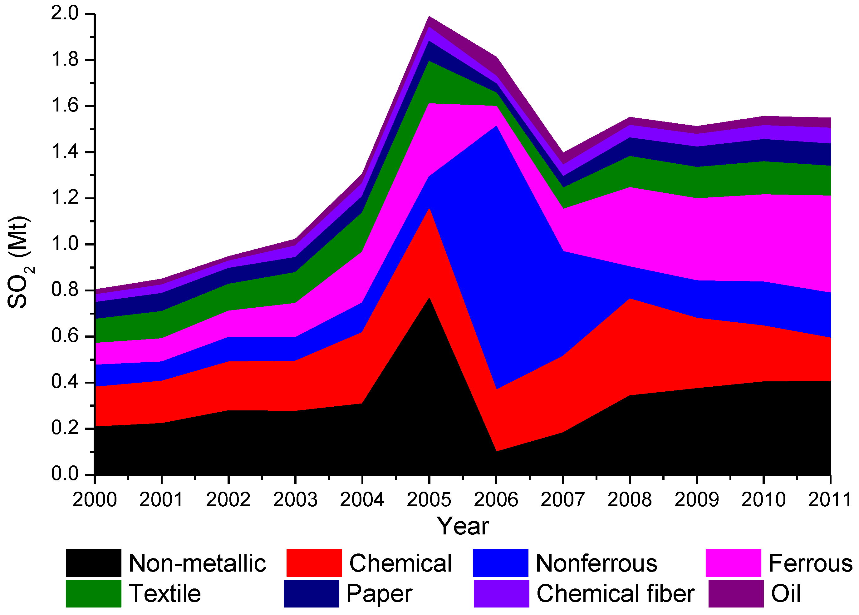
3.1. Temporal Variations of SO2 Emissions

Based on the temporal trend of the total SO2 emissions in Jiangsu province, the study period can be divided into three phases (Figure 3): a typical increase from 2000–2005, a typical decrease, except the chemical and non-ferrous subsector, from 2005–2008 and, then, a slow increase, except the chemical subsector, from 2008–2011. However, different trends were observed for each separate subsector (Figure 3). From 2000–2011, SO2 emissions increased tremendously in the non-ferrous subsector by 346.0%. From 2005–2011, emissions in non-metallic, chemical, textile and oil sectors decreased by 10.5%–39.0%. From 2008–2011, emissions decreased only in the chemical and textile sectors by 55.4% and 4.5%, respectively. This indicates that SO2 emissions have been controlled effectively in the chemical and textile subsectors, while related measures should be strengthened further to reduce SO2 emissions in the other six subsectors, especially for non-metallic, non-ferrous and ferrous subsectors.

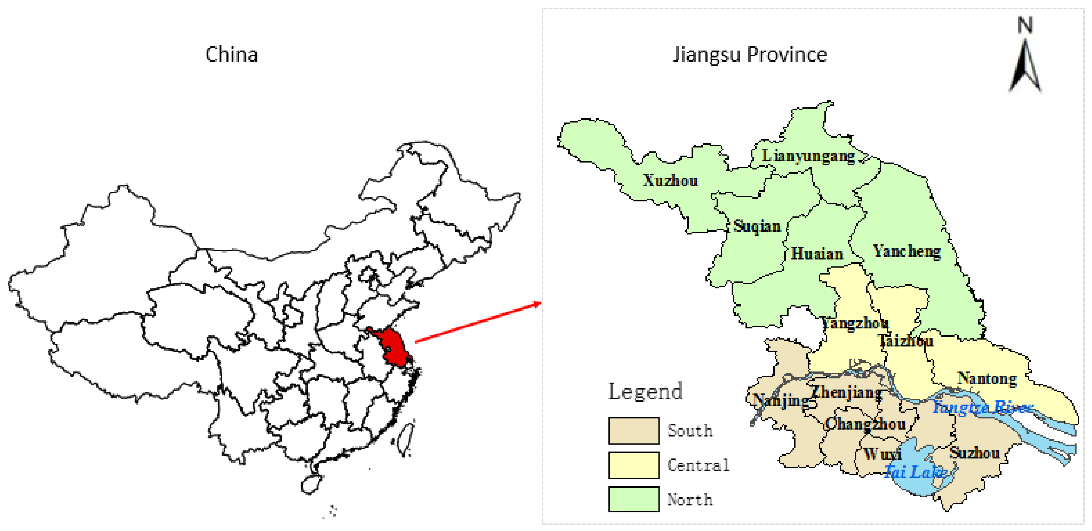
3.2. Spatial Variations of Regional SO2 Emissions

During the period of 2000–2011, the south region was the main contributor, accounting for ~70% of the total SO2 emissions, and the other two regions contributed a similar amount (Figure 4). Emissions declined in the three regions since 2006. Before 2008, there was a similar trend in SO2 emissions among the three regions. During 2008–2011, an increasing trend was found in the north, while decreasing trends happened in the other two regions.
In terms of subsectors (Figure 5), SO2 emissions declined only in the southern chemical and textile subsectors and the central chemical fiber subsector, while the emissions in the ferrous subsector increased by 320.9%, 305.4% and 690.0% in the south, central and north, respectively, from 2000–2011. During 2005–2011, the emissions of the non-metallic sector declined in the three regions, of the chemical subsector decreased in the south and north, of the oil subsector also declined in the south and central and of the textile and chemical fiber subsectors declined in the south and central. During 2008–2011, SO2 emissions declined only in the southern chemical and textile subsectors, the central chemical subsector and the northern chemical subsector, with a reduction rate of 60.1%, 16.5%, 52.0% and 37.8%, separately. This led to different SO2 emission fractions from each region between the three time periods of 2000–2005, 2005–2008 and 2008–2011. Emission ratios declined in the southern subsectors, except chemical fiber, increased in the central ones, expect ferrous, and increased in the northern ones, respectively, from the first period (2000–2005) to the third period (2008–2011). Hence effective measures should be implemented on the ferrous, non-ferrous, chemical fiber and oil subsectors for SO2 reduction in the province.
Generally, SO2 emissions from the manufacturing industry had significant regional differences in Jiangsu province, which was similar to the industrial SO2 emissions in Jiangsu [56] and the national trend in China [57,58].

3.3. Decomposition Analysis of SO2 Emissions

To further analyze the characteristics of regional SO2 emissions, its sector decomposition is studied using Equations (5)–(9), and the results are shown in Table 3, Table 4 and Table 5, respectively. A negative value means emission-reduction from the calculation year to the base year. The value does not represent the absolute increase/decrease amount of SO2 emissions. For instance, the cleaner production technology effect reflects the contribution of the technology factor to the emissions change between the calculation year and the base year, not the absolute reduction amount of SO2 emissions due to technology in the calculation year.
In the whole province, the inter-annual fluctuations and the decompositions of SO2 emissions are shown in Table 3. Ieffect contributed to reduced emissions, while both Reffect and Seffect acted as the same contribution in some specific years, e.g., Reffect had a removal rate of 83.0% and made SO2 decline by 0.042 Mt during 2006–2007. Veffect always made a negative contribution to emission reduction. Such a contribution caused an inverted U-shaped curve for time vs. SO2 emissions. The peak of this curve was 0.031 Mt in 2005. Table 3 also shows that the inter-annual emissions (ΔE) were negative in 2006, 2007, 2009 and 2011. In 2006 and 2011, Ieffect also contributed to reduced emissions with removal rates of 95.3% and 100%, respectively. In 2007 and 2009, the combined actions of both Ieffect + Reffect and Ieffect + Seffect reduced the emissions. Moreover, Seffect always played an important role in the emission reduction, which was closely associated with the 2008 financial crisis.
As for regional decomposition (Table 4), Ieffect also contributed to reduced emissions, while Veffect was the opposite. Reffect and Seffect acted as different contributions to the emission reductions in the three regions during the different periods of 2000–2005, 2005–2008 and 2008–2011. In the south, Reffect caused a 0.376-Mt SO2 emission reduction with a removal ratio of 37.5% during the period 2005–2008, while Veffect contributed to increased emissions during the three periods. In the central region, the reduction contributions were 4.1% for Reffect during 2005–2008 and 22.9% for Seffect during 2008–2011. In the north, Reffect had a removal ratio of 54.8% during 2005–2008, and Veffect increased the emissions during the three periods. Though Ieffect cut down 0.126 Mt, ΔE increased 0.074 Mt during 2008–2011. For the overall SO2 emission reductions, the combined action of Ieffect + Reffect achieved a reduction during 2005–2008, while that of Ieffect + Seffect achieved this during 2008–2011.
In all manufacturing subsectors (Table 5), Ieffect also played a key role in reducing the SO2 emissions in the chemical and ferrous subsectors. The combined effects of Ieffect + Seffect and Ieffect + Reffect reduced the emissions effectively in the textile and non-ferrous subsectors, respectively, especially in the two periods of 2000–2005 and 2005–2008. The combined three effects of Ieffect, Seffect and Reffect decreased the emissions in three out of the other four subsectors. Table 5 also shows negative values of the inter-period emissions in manufacturing sectors, except the ferrous sector during 2005–2011. The negative values were found in the non-metallic, non-ferrous, textile, paper, chemical fiber and oil subsector during 2005–2008 and in the chemical and textile subsectors during 2008–2011. This also indicated that the period of SO2 emission reduction mainly appeared during 2005–2008. However, during 2008–2011, the inter-period SO2 emissions increased mainly for Reffect, which contributed to reduced emissions, especially in the chemical and paper subsectors. Moreover, Seffect did not fulfill itself in the emission reduction, especially for the non-metallic, chemical, chemical fiber and oil subsectors.

3.4. Characteristics of Manufacturing Transfer

Using the shift-share model, the competitive component D values of the non-metallic, chemical, non-ferrous, ferrous, textile, paper, chemical fiber and oil subsectors are calculated and shown in Figure 6. There are different agglomerations for different manufacturing subsectors in the south, central and north during the three periods of 2000–2005, 2005–2008 and 2008–2011.
During 2000–2005, most of the D values for the eight subsectors were positive in the south and negative in the north, indicating that these subsectors had not been transferred from the central and north to the south. During that period, manufacturing, especially for the chemical subsector in the south, was booming for the regional developments along the Yangtze River and along the Hu-Ning expressway, while the center and north regions were left for further development [27]. Thus, it could be concluded that those subsectors, such as the chemical, chemical fiber, textile and ferrous subsectors, are clustering and had a stronger competitive advantage in the south, which is attributed to the transfer from other developed regions outside the province, such as Shanghai and foreign countries [59]; while in the north, the industrial economic level was low and the industrial structure was simple, which led to the negative D values. The clustering pattern changed since 2005, which was attributed to regional policies, such as the industry belt along Long-Hai railway and the Advices of Promoting Industrial South-North Transfer in Jiangsu Province after 2004 [27].
During 2005–2008, the estimated D values for these five subsectors (non-metallic, chemical, non-ferrous, ferrous, textile, paper sector) were negative in the south and the opposite in the central and north, from which we can conclude that these subsectors, especially the chemical and textile sector had, transferred from the south to the central and north (Table 6). D values of chemical subsector accounted for −58.1% of the total negative D values in the south, while 38.9% and 19.3% of the total positive D values in the central and north, respectively. D values of the textile subsector accounted for −31.2% of the total negative D values in the south, while 19.1% and 12.1% of the total positive D values in the central and north, respectively. As for the chemical fiber subsector, the positive D values were found in the south and north, and the former was larger, which indicated that the chemical fiber subsector still had a stronger competitive advantage in the south. D values of the oil subsector were negative and only accounted for 0.04% and 1.2% of their total negative D values in the south and central, respectively. In the north, all of the D values in the eight subsectors were positive. The D value of the oil subsector was 0.24 RMB billion, accounted for 0.4% of the total positive D value, indicating that the oil subsector somewhat transferred from the south and central to the north. In total, these five subsectors of the non-metallic, chemical, non-ferrous, ferrous, textile and paper sector had an absolute competitive ability in the central and north and had been transferred from the south to the central and north during 2005–2008.
During 2008–2011, following the preceding developmental tendency of manufacturing subsectors, some subsectors, such as the non-metallic, non-ferrous, ferrous, paper, chemical fiber and oil subsector in the central, were transferred to the north, and the first three subsectors accounted for 20.4%, 36.0% and 30.5% of the total negative D values in the central (Figure 6 and Table 6). In the south, chemical and textile sectors also were the main transfer sectors; their D values contributed −55.5% and −30.2% to the total negative D value, respectively. In the north, seven D values in the eight subsectors were positive, and the D values of the chemical, ferrous and textile sectors contributed 31.8%, 23.4% and 14.8% to the total positive D value, respectively. This indicates that chemical and textile subsectors continued to be transferred from the south to the central and north while the ferrous sector transferred from the south and central to the north during 2008–2011.
Compared to the D values (Figure 6 and Table 6) and the official data on the transfer of enterprise (Table 1 and Table 2), the result could be deduced that the chemical and textile subsectors were typical and had been transferred from the south to the central and north during 2005–2011. The ferrous sector began to transfer from the central to the north during 2008–2011.

3.5. SO2 Emissions for Manufacturing Transfer

Based on Section 3.4, manufacturing transfer was only found in the south during 2000–2005, while the pattern was formed that manufacturing subsectors transferred from the south to the Central and north during 2005–2008 and 2008–2011. Therefore, the SO2 emissions of the manufacturing transfer during the two periods were estimated by Equation (11) and are shown in Table 7.
During 2005–2008, SO2 emissions in the south transferred out −13.26 Mt, which were transferred as 6.31 and 6.97 Mt to the central and north, respectively. The non-metallic and chemical subsectors were the main SO2 emission transfer subsectors. The former SO2 emissions were mainly transferred from the south (3.50 Mt) to the north (2.66 Mt), while the latter mainly from the south (5.11 Mt) to the central (3.42 Mt), respectively.
During 2008–2011, SO2 emissions in the south kept transferring out, and its emissions were −6.58 Mt. Some subsectors, such as the non-metallic, non-ferrous, ferrous, paper, chemical fiber and oil subsector, began to transfer from the central, and its SO2 emissions were −2.23 Mt. SO2 emissions only in the chemical and textile sectors were still transferred to the central with 0.30 and 0.32 Mt, respectively. In the north, there were 7.46 Mt SO2 emissions, which were from the south and central. In that period, these subsectors, including the non-metallic and ferrous subsectors in the south and the non-metallic and non-ferrous subsectors in the central, had larger SO2 emissions that were transferred out. Certainly, the north had 4.63 Mt emissions transferred only from the non-metallic and ferrous subsectors, which accounted for 62.1% of the total SO2 emissions transferred in (7.46 Mt).
Accounting to all of the transferred SO2 emissions of the eight subsectors transferred together, the south, central and north showed −12.36, 5.36 and 6.97 Mt during 2005–2008 and −5.62, −1.60 and 7.23 Mt during 2008–2011, respectively (Table 7). It could be concluded that SO2 emissions were of the same amount for the transfer-in and transfer-out in the same period. Thus, 43.4% and 56.4% SO2 emissions in the south were transferred to the central and north during 2005–2008, respectively. Additionally, 77.7% of the transfer-in SO2 emissions in the north were from the south and 22.1% from the central during 2008–2011, respectively.

4. Discussion

In the eight typical manufacturing subsectors, the total SO2 emissions increased from 0.99 Mt in 2000 to 1.82 Mt in 2011, though the emissions decreased by 22.1% from 2005–2011 in Jiangsu province. The increasing trend for the total SO2 emissions was in agreement with the trend of SO2 deposition [60]. Meanwhile, regional nitrogen emissions and depositions also increased [60,61,62]. This changed the compositions of acid rain [63,64] and brought a new challenge for the regional eco-environment and the regional economies [26,65,66].
During 2000–2011, SO2 emissions had similar variations, but there was a sharp reduction during 2005–2007. As for the manufacturing transfer and related SO2 emissions, those for the south and the central happed during 2005–2008 and 2008–2011, respectively. The reasons for the above variations of SO2 emissions are considered complicated and intertwined:
(1) Industrial policies: The policy “Temporary Regulation of Promoting Industrial Structure Adjustment, Advices of Promoting Industrial South-North Transfer in Jiangsu Province, and the Catalogue of Industrial Structure Adjustment” was unveiled in 2005. A series of circulars on industrial structure adjustments were then passed in the chemical (soda and coal), non-metallic (cement), non-ferrous (Al and Cu), ferrous (Fe) and textile subsectors in 2006. The Circular on Strict Enforcements of Entry Conditions in tungsten (W), tin (Sn) and antimony (Sb) subsectors was issued in January 2007. The Cement Approval Conditions of Jiangsu Province was also passed in August 2007. These policies led to important SO2 emission reductions, especially in the textile subsector, during 2007–2010 (Table 3, Table 4 and Table 5) and related subsectors transferred from the south to the central and north (Figure 6 and Table 6).
(2) Unforeseen conditions: In 2007, the Lake Taihu water pollution incident occurred. Since its pollution sources were located in the south, such as Wuxi, Changzhou and Suzhou, parts of high-energy-consuming and heavy-polluting industries, such as the textile, chemical, ferrous and non-metallic subsectors, were forced to relocate to the north, such as Suqian, Lianyungang and Yancheng. In 2008, the global financial crisis broke out and also negatively impacted the whole manufacturing sector in Jiangsu province. Many factories in the south or central were forced to suspend operations, declare bankruptcy or relocated to the central or north. Meanwhile, to achieve the target of a high GDP ratio and against the financial crisis, both governments and businessmen paid more attention to GDP and made measures to expand domestic demand even more to promote the development of the domestic market, but in the moving process, pollution emissions were neglected, especially in pollution abatements. These might be important reasons that SO2 emissions had a sharp reduction in 2007 and that the higher shift-share values occurred during 2005–2008, especially in the chemical and textile subsectors (Figure 4, Figure 5 and Figure 6 and Table 3, Table 4 and Table 5).
(3) Environmental policies: The “Notice on Chemical Industry Pollution Treatments in the Taihu Lake Basin, Jiangsu Province” and the “Proposals of further promoting the Level of Environmental Protection and Construction in the Development Areas in Jiangsu Province” were made in 2005. The “Proposals of strengthening Eco-Environmental Protection” and the “Construction and Notice on a Work Program of Taihu Lake Pollution Treatments” were issued in 2006 and 2007, respectively. A “Regional Compensatory Approach of Environment Resources in Jiangsu Province I and Circular of Environmental Protection and Eco-construction Plan (2006–2010)” was issued in 2008. These policies improved the regional environment and the industrial structure, especially in the south, and further promoted manufacturing transfer to inner Jiangsu province.
(4) Government actions: The government played a leading role in the environmental protection, but in many cases, the government was also the cause of environmental degradation [67]. Furthermore, the government created sound conditions for regional industrial development by implementing “top-down” macro-policies that focused development on selected subsectors and regions [68]. Regardless of the SO2 emission reduction or the manufacturing transfer, the government would play an important role without dispute [68,69].

5. Conclusions

The manufacturing SO2 emissions in Jiangsu province still increased during 2000–2011, though the emissions had a reduction during 2005–2010. Regionally, the south was the main region for SO2 emissions and dominated the total emission trend of the whole of Jiangsu province. During 2000–2011, the cleaner production level contributed to reducing the SO2 emissions, while the industrial scale level was the opposite. The output structure level had not fully played its role in decreasing the emissions. Both the levels of the output structure and pollution abatement played key roles in specific years. For the regional manufacturing development, the south was the transfer-in region during 2000–2005 and then changed into the transfer-out region during 2005–2011. The central was the transition zone, with a transfer-in period of 2005–2008 and a partial transfer-out period of 2008–2011. Additionally, the north was the main transfer-in region during 2005–2011. Because of the manufacturing transfer, the central region transferred in 43.4% of the south’s emissions during 2005–2008. The north region transferred in 56.4% and 77.7% of the south’s emissions during 2005–2008 and 2008–2011, respectively, and 22.1% of the central’s emissions during 2008–2011. Manufacturing transfer redistributed environmental pollution spatially, and the damage to the ecological environment during the manufacturing transfer needs to be controlled.

Acknowledgments

This work is jointly founded by the Program of Development and Strategic Planning, Nanjing Institute of Geography & Limnology, Chinese Academy of Sciences (NIGLAS2012135006) and the National Natural Science Foundation of China (41571461, 41201206). Many thanks are given to Leiming Zhang, who is employed by Environment Canada, and to the editors and the anonymous reviewers for their valuable comments and suggestions on this study.

Author Contributions

All the authors conceived and designed the research for this study. Ying Peng, Jian Cui and Ying Du did the analysed model data. Ying Peng prepared the first version of the manuscript. All the authors together supervised the analysis and contributed to the revision of the manuscript.

Conflicts of Interest

The authors declare no conflict of interest.

Appendix

Table A1. Changes of SO2 emission intensity (ei) in the seven industrial subsectors of Jiangsu province (unit: t/1000 RMB).
200020012002200320042005200620072008200920102011
Non-metallic0.5290.4950.5580.5470.4890.4200.1180.1800.2760.2430.2140.188
Chemical0.1650.1630.1550.1330.1510.1440.0830.0860.0880.0570.0360.023
Non-ferrous0.4200.3390.3810.2750.2480.1980.2000.3020.0930.0920.0910.090
Ferrous0.2060.1750.1520.1220.1110.1210.0280.0450.0740.0730.0730.072
Textile0.0850.0880.0750.0740.0810.0710.0190.0270.0390.0360.0340.031
Paper0.3880.3540.2570.2220.2140.2140.0840.1010.1210.1200.1190.117
Chemical fiber0.1220.1270.0930.1150.1000.0880.0400.0490.0610.0550.0500.045
Oil0.0880.0950.0830.0870.0960.0860.1280.0750.0440.0410.0370.034

References

  1. Wang, Y.; Wang, M.H.; Zhang, R.Y.; Ghan, S.J.; Lin, Y.; Hu, J.X.; Pan, B.W.; Levy, M.; Jiang, J.H.; Molina, M.J. Assessing the effects of anthropogenic aerosols on Pacific storm track using a multiscale global climate model. PNAS 2014, 111, 6894–6899. [Google Scholar] [CrossRef] [PubMed]
  2. Dotse, S.Q.; Dagar, L.; Petra, M.I.; De Silva, L.C. Evaluation of national emissions inventories of anthropogenic air pollutants for Brunei Darussalam. Atmos. Environ. 2016, 133, 81–92. [Google Scholar] [CrossRef]
  3. Geng, Y.; Wei, Y.M.; Fischedick, M.; Chiu, A.; Chen, B.; Yan, J.Y. Recent trend of industrial emission in developing countries. Appl. Energy 2016, 166, 187–190. [Google Scholar] [CrossRef]
  4. Zhang, J.; Hu, W.; Wei, F.; Wu, G.; Korn, L.R.; Chapman, R.S. Children’s respiratory morbidity prevalence inrelation to air pollution in four Chinese cities. Environ. Health Perspect. 2002, 110, 961–967. [Google Scholar] [CrossRef] [PubMed]
  5. Wong, M.C.S.; Tam, W.W.S.; Wang, H.H.X.; Lao, X.X.; Zhang, D.D.; Chan, S.W.M.; Kwan, M.W.M.; Fan, C.K.M.; Cheung, C.S.K.; Tong, E.L.H.; et al. Exposure to air pollutants and mortality in hypertensive patients according to demopraphy: A 10 year case-crossover study. Environ. Pollut. 2014, 192, 179–185. [Google Scholar] [CrossRef] [PubMed]
  6. Jochner, S.; Markevych, I.; Beck, I.; Traidl-Hoffmann, C.; Heinrich, J.; Menzel, A. The effects of short- and long-term air pollutants on plant phenology and leaf characteristics. Environ. Pollut. 2015, 206, 382–389. [Google Scholar] [CrossRef] [PubMed]
  7. Sun, Y.L.; Zhuang, G.; Huang, K.; Li, J.; Wang, Q.; Wang, Y.; Lin, Y.; Fu, J.; Zhang, W.; Tang, A.; et al. Asian dust over northern China and its impact on the downstream aerosol chemistry in 2004. J. Geophys. Res. 2010, 115, 3421–3423. [Google Scholar] [CrossRef]
  8. Dou, J.; Shen, Y.B. On the influence of the industrial transfer on the environment in the Central region of China. China Popul. Resour. Environ. 2014, 24, 96–102. (In Chinese) [Google Scholar]
  9. Liang, H.W.; Dong, L.; Luo, X. Balancing regional industrial development: Analysis on regional disparity of China’s industrial emissions and policy implications. J. Clean. Prod. 2016, 126, 223–235. [Google Scholar] [CrossRef]
  10. Dong, L.; Liang, H.W. Spatial analysis on China’s regional air pollutants and CO2 emissions: Emission pattern and regional disparity. Atmos. Environ. 2014, 92, 280–291. [Google Scholar] [CrossRef]
  11. Sharma, D.; Kulshrestha, U.C. Spatial and temporal patterns of air pollutants in rural and urban areas of India. Environ. Pollut. 2014, 195, 276–281. [Google Scholar] [CrossRef] [PubMed]
  12. Jiangsu Provincial Bureau of Statistic (JSPBS) 2007–2013. Available online: http://www.jssb.gov.cn/tjxxgk/tjsj/tjnq/jstjnj2014/index_212.html (accessed on 16 May 2016).
  13. Han, M.; Wang, T.J.; Xu, R.L. Present and future situation of air pollution and acid rain in Jiangsu province. Pollut. Control Technol. 2003, 16, 17–20. (In Chinese) [Google Scholar]
  14. Hou, F.Q. A study on environmental impact of regional economy concentration in China. J. Northwest A F Univ. (Soc. Sci. Ed.) 2008, 8, 20–25. (In Chinese) [Google Scholar]
  15. Fu, X.; Wang, S.X.; Zhao, B.; Xing, J.; Cheng, Z.; Liu, H.; Hao, J.M. Emission inventory of primary pollutants and chemical speciation in 2010 for the Yangtze River Delta region, China. Atmos. Environ. 2013, 70, 39–50. [Google Scholar] [CrossRef]
  16. Zhao, Y.; Wang, S.; Duan, L.; Lei, Y.; Cao, P.; Hao, J.M. Primary air pollutant emissions of coal-fired power plants in China: Current status and future prediction. Atmos. Environ. 2008, 42, 8442–8452. [Google Scholar] [CrossRef]
  17. Tian, J.; Shi, H.; Chen, Y.; Chen, L. Assessment of industrial metabolisms of sulphur in a Chinese fine chemical industrial park. J. Clean. Prod. 2012, 32, 262–272. [Google Scholar] [CrossRef]
  18. Liu, Y.X. Damage effects of SO2 and its epidemiology and toxicology research. Asian J. Ecotoxicol. 2007, 2, 225–231. (In Chinese) [Google Scholar]
  19. Horaginamani, S.M.; Ravichandran, M. Ambient air quality in an urban area and its effects on plant and human beings: A case study of Tiruchirappalli, India. Ravichandran Kathmandu Univ. J. Sci. Eng. Tech. 2010, 6, 13–19. [Google Scholar] [CrossRef]
  20. Su, S.; Li, B.; Tao, S. Sulfur dioxide emissions from combustion in China: From 1990 to 2007. Environ. Sci. Technol. 2010, 45, 8403–8410. [Google Scholar] [CrossRef] [PubMed]
  21. Fujii, H.; Managi, S.; Kaneko, S. Decomposition analysis of air pollution abatement in China: Empirical study for ten industrial sectors from 1998 to 2009. J. Clean. Prod. 2013, 59, 22–31. [Google Scholar] [CrossRef]
  22. Dong, L.; Dong, H.J.; Fujita, T.; Geng, Y.; Fujii, M. Cost-effectiveness analysis of China’s SO2 control strategy at the regional level: Regional disparity, inequity and future challenges. J. Clean. Prod. 2015, 90, 345–359. [Google Scholar] [CrossRef]
  23. Cui, J.; Zhou, J.; Peng, Y.; He, Y.Q.; Yang, H.; Xu, L.J.; Chan, A. Long-term atmospheric wet deposition of dissolved organic nitrogen in a typical red-soil agro-ecosystem, Southeastern China. Environ. Sci. Proc. Impact 2014, 16, 1050–1058. [Google Scholar] [CrossRef] [PubMed]
  24. Lu, W.C.; Li, Y.L. Research on driving factors of China’s industrial emissions abatement: An empirical study based on a LMDI method. Stat. Inform. Forum 2010, 25, 49–54. (In Chinese) [Google Scholar]
  25. Xu, Y.; Williams, R.H.; Socolow, R.H. China’s rapid deployment of SO2 scrubbers. Energy Environ. Sci. 2009, 2, 459–465. [Google Scholar] [CrossRef]
  26. Hering, L.; Poncet, S. Environmental policy and exports: Evidence from Chinese cities. J. Environ. Econ. Manag. 2014, 68, 296–318. [Google Scholar] [CrossRef]
  27. Qiu, F.D.; Tang, X.D.; Zhang, C.M.; Zhu, C.G.; Yao, X.W. Characteristic and mechanism of spatial-temporal differentiation in Jiangsu province during the period of industrial transformation. Geogr. Res. 2015, 34, 787–800. (In Chinese) [Google Scholar]
  28. Fan, M.Y.; Shen, Z.P. Analysis on spatial pattern and its change of manufacturing industry in Jiangsu province. J. Jiangsu Norm. Univ. (Nat. Sci. Ed.) 2014, 32, 63–67. (In Chinese) [Google Scholar]
  29. Wang, Z.H.; Chen, Q. Synthetic measure on the structure upgrading of manufacturing in Jiangsu. Ecol. Econ. 2012, 4, 99–103. (In Chinese) [Google Scholar]
  30. Xu, L.D. Environmental ethical review on industrial transferring and undertaking. J. Kunming Univ. Sci. Technol. 2010, 10, 1–5. (In Chinese) [Google Scholar]
  31. Jin, X.R.; Tan, L.L. Differences in environmental policies and transfer of regional industry: A perspective of new economic geography. J. Zhejiang Univ. (Humanities Soc. Sci.) 2012, 42, 51–60. (In Chinese) [Google Scholar]
  32. Jiangsu Development and Reform Commission. Available online: http://www.jsdpc.gov.cn/gongkai/wjg/sbb/gzdt/index_55.html (accessed on 16 May 2016).
  33. Wang, Y.G.; Ying, Q.; Hu, J.L.; Zhang, H.L. Spatial and temporal variations of six criteria air pollutants in 31 provincial capital cities in China during 2013–2014. Environ. Int. 2014, 73, 413–422. [Google Scholar] [CrossRef] [PubMed]
  34. Tao, Z.M.; Hewings, G.; Donaghy, K. An economic analysis of Midwestern US criteria pollutant emissions trends from 1970 to 2000. Ecol. Econ. 2010, 69, 1666–1674. [Google Scholar] [CrossRef]
  35. He, J. What is the role of openness for China’s aggregate industrial SO2 emission? A structural analysis based on the Divisia decomposition method. Ecol. Econ. 2009, 69, 868–886. [Google Scholar] [CrossRef]
  36. Liu, Q.L.; Wang, Q. Pathways to SO2 emissions reduction in China for 1995–2010: Based on decomposition analysis. Environ. Sci. Policy 2013, 33, 405–415. [Google Scholar] [CrossRef]
  37. Ang, B.W. Decomposition analysis for policymaking in energy: Which is the preferred method? Energy Policy 2004, 32, 1131–1139. [Google Scholar] [CrossRef]
  38. Ang, B.W. The LMDI approach to decomposition analysis: A practical guide. Energy Policy 2005, 33, 867–871. [Google Scholar] [CrossRef]
  39. Zotter, K.A. “End-of-pipe” versus “Process-integrated” water conservation solutions—A comparison of planning, implementation and operating phases. J. Clean. Prod. 2004, 12, 685–695. [Google Scholar] [CrossRef]
  40. Cao, F.Z. Foreign Environmental Development Strategy Research; Environmental Science Press: Beijing, China, 1993. [Google Scholar]
  41. Hitchens, D.; Trainor, M.; Clausen, J.; De Marchi, S.T.B. Small and Medium Sized Companies in Europe—Environmental Performance. Competitiveness and Management; Springer Verlag: Berlin, Germany, 2003. [Google Scholar]
  42. Rennings, K.; Kemp, R.; Bartolomeo, M.; Hemmelskamp, J.; Hitchens, D. Blueprints for an Integration of Science, Technology and Environmental Policy; Centre for European Economic Research (ZEW): Mannheim, Germany, 2004. [Google Scholar]
  43. Rennings, K.; Ziegler, A.; Zwick, T. Employment Changes in Environmentally Innovative Firms. Available online: http://papers.ssrn.com/sol3/papers.cfm?abstract_id=329120 (accessed on 16 May 2016).
  44. Ke, J. Legal discussion on promoting cleaner production in China. China Soft Sci. 2000, 9, 25–28. (In Chinese) [Google Scholar]
  45. Wang, L.P.; Yu, X.L. The development of clean production and end treatment. China Popul. Resour. Environ. 2010, 20, 428–431. (In Chinese) [Google Scholar]
  46. De Bruyn, S.M. Explaining the environmental Kuznets curve: Structural change and international agreements in reducing sulphur emissions. Environ. Dev. Econ. 1997, 2, 485–503. [Google Scholar] [CrossRef]
  47. Copeland, B.R.; Taylor, M.S. North-south trade and the environment. Quart. J. Econ. 1994, 109, 755–787. [Google Scholar] [CrossRef]
  48. Peters, G.P. From production-based to consumption-based national emission inventories. Ecol. Econ. 2008, 65, 13–23. [Google Scholar] [CrossRef]
  49. Stern, D.I. Explaining changes in global sulphur emissions: An econometric decomposition approach. Ecol. Econ. 2002, 42, 201–220. [Google Scholar] [CrossRef]
  50. Grossman, G.M.; Krueger, A.B. Economic growth and the environment. Q. J. Econ. 1995, 110, 353–377. [Google Scholar] [CrossRef]
  51. Vukina, T.; Beghin, J.C.; Solakoglu, E.G. Transition to markets and the environment: Effects of the change in the composition of manufacturing output. Environ. Dev. Econ. 1999, 4, 582–598. [Google Scholar] [CrossRef]
  52. Bruvoll, A.; Medin, H. Factors behind the environmental Kuznets curve: A decomposition of the changes in air pollution. Environ. Resour. Econ. 2003, 24, 27–48. [Google Scholar] [CrossRef]
  53. Shi, C.Y.; Zhang, J.; Yang, Y.; Zhou, Z. Shift-share analysis on international tourism competitiveness—A case of Jiangsu province. Chin. Geogr. Sci. 2007, 17, 173–178. [Google Scholar] [CrossRef]
  54. Chen, W.; Xu, J.P. An application of shift-share model to economic analysis of county. Word J. Model. Simul. 2007, 3, 90–99. [Google Scholar]
  55. Ministry of Environmental Protection of the People’s Republic of China (MEPPRC) 2010. Available online: http://www.mep.gov.cn/zhxx/hjyw/201002/t20100210_185661.htm (accessed on 16 May 2016).
  56. Zhao, X.F.; Huang, X.J.; Zhang, X.Y.; Zhu, D.M.; Lai, L.; Zhong, T.Y. Application of spatial autocorrelation analysis to the COD, SO2 and TSP emission in Jiangsu province. Environ. Sci. 2009, 30, 1580–1587. (In Chinese) [Google Scholar]
  57. Gao, C.L.; Yin, H.Q.; Ai, N.S.; Huang, Z.W. Historical analysis of SO2 pollution control policies in China. Environ. Manag. 2009, 43, 447–457. [Google Scholar] [CrossRef] [PubMed]
  58. Li, M.S.; Ren, X.X.; Zhou, L.; Zhang, F.Y.; Zhang, J.H. Spatial mismatch between SO2 pollution and SO2 emission in China. Acta Sci. Circumst. 2013, 33, 1150–1157. (In Chinese) [Google Scholar]
  59. Sun, J.; Yao, J.F. Empirical study on contribution of industry transfer to Jiangsu economic development- by the example of Southern-Northern Co-building Industrial Parks. Econ. Geogr. 2011, 31, 432–436. [Google Scholar]
  60. Cui, J.; Zhou, J.; Peng, Y.; He, Y.Q.; Yang, H.; Mao, J.D.; Zhang, M.L.; Wang, Y.H.; Wang, S.W. Atmospheric wet deposition of nitrogen and sulfur in the agroecosystem in developing and developed areas of Southeastern China. Atmos. Environ. 2014, 89, 102–108. [Google Scholar] [CrossRef]
  61. Tian, Y.H.; Yang, L.Z.; Yin, B.; Zhu, Z.L. Wet deposition N and its runoff flow during wheat seasons in the Tai lake region, China. Agric. Ecosyst. Environ. 2011, 141, 224–229. [Google Scholar] [CrossRef]
  62. Qiao, X.; Tang, Y.; Hu, J.L.; Zhang, S.; Li, J.Y.; Kota, S.H.; Wu, L.; Guo, H.L.; Zhang, H.L.; Ying, Q. Modeling dry and wet deposition of sulfate, nitrate, and ammonium ions in Jiuzhaigou National Nature Reserve, China using a source-oriented CMAQ model: Part I. Base case model results. Sci. Total Environ. 2015, 532, 831–839. [Google Scholar] [CrossRef] [PubMed]
  63. Song, G.J.; Qian, W.T.; Ma, B.; Zhou, L. Preliminary evaluation on the policies of acid rain control in China. China Popul. Resour. Environ. 2013, 23, 6–12. (In Chinese) [Google Scholar]
  64. Fang, Y.T.; Wang, X.M.; Zhu, F.F.; Wu, Z.Y.; Li, J.; Zhong, L.J.; Chen, D.H.; Yoh, M. Three-decade changes in chemical composition of precipitation in Guangzhou city, southern China: Has precipitation recovered from acidification following sulphur dioxide emission control? Tellus B 2013, 65, 20213. [Google Scholar] [CrossRef]
  65. Yuan, X.L.; Mi, M.; Mu, R.; Zuo, J. Strategic route map of sulphur dioxide reduction in China. Energy Policy 2013, 60, 844–851. [Google Scholar] [CrossRef]
  66. Wei, J.C.; Guo, X.M.; Marinova, D.; Fan, J. Industrial SO2 pollution and agricultural losses in China: Evidence from heavy air polluters. J. Clean. Prod. 2014, 64, 404–413. [Google Scholar] [CrossRef]
  67. Li, Z.P. On the government’s environmental responsibility and liability-based on the government responsibility for the environmental quality. J. China Univ. Geosci. (Soc. Sci. Ed.) 2008, 8, 37–41. (In Chinese) [Google Scholar]
  68. Wei, Y.H.; Fan, C. Regional inequality in China: A case study of Jiangsu province. Prof. Geogr. 2000, 52, 455–469. [Google Scholar] [CrossRef]
  69. Taylor, M.R.; Rubin, E.S.; Hounshell, D.A. Effect of government actions on technological innovation for SO2 control. Environ. Sci. Technol. 2003, 37, 4527–4534. [Google Scholar] [CrossRef] [PubMed]
Figure 1. The study area, Jiangsu province, grouped into three regions: south, central and north. The south is the developed region, which includes Suzhou, Wuxi, Changzhou, Nanjing and Zhenjiang; the central is the developing region, which includes Yangzhou, Taizhou and Nantong; and the north is the undeveloped region, which includes Xuzhou, Suqian, Huai’an, Lianyungang and Yancheng.
Atmosphere 07 00069 g001
Figure 2. Variations of industrial SO2 emissions in the excavation, manufacturing and power and heating industries from a survey dataset in Jiangsu province during 2000–2012 (JSPBS, Jiangsu Provincial Bureau of Statistic, 2011–2013) [12].
Atmosphere 07 00069 g002
Figure 3. Temporal variations of SO2 emissions of different manufacturing sectors in Jiangsu province during 2000–2011.
Atmosphere 07 00069 g003
Figure 4. Spatial variations of total SO2 emissions of manufacturing in Jiangsu province during 2000–2011.
Atmosphere 07 00069 g004
Figure 5. Spatial variations of the SO2 emissions of different manufacturing subsectors in Jiangsu province during 2000–2011.
Atmosphere 07 00069 g005
Figure 6. D values in individual subsectors in the three regions during 2000–2011.
Atmosphere 07 00069 g006
Table 1. The number of all transferred enterprises by different pathways from the south to the north of Jiangsu during 2006–2010.
TimeTotalLine DepartmentsIntegral EnterpriseMarketing, R&D Departments
2006291278013
2008417397910
20103563251120
Note: data were calculated using the available website [32].
Table 2. The number of transfer enterprises in the eight subsectors from the south to north during 2006–2010.
YearNon-MetallicChemicalNon-FerrousFerrousTextilePaperChemical FiberOilSummation
2006146512212820115
200714728813130119
2008208961123700156
2010309971225070180
Note: data were calculated using the available website [32].
Table 3. Decomposition results of SO2 emission changes in Jiangsu province (unit: Mt).
TimeΔE R e f f e c t I e f f e c t S e f f e c t V e f f e c t
2000–20010.046−0.001 (1.6%)−0.049 (90.4%)−0.004 (8.0%)0.101
2001–20020.098−0.059 (76.3%)0.017−0.018 (23.7%)0.158
2002–20030.075−0.022 (13.3%)−0.079 (47.6%)−0.065 (39.1%)0.241
2003–20040.2830.022−0.044 (100%)0.0120.294
2004–20050.684−0.110 (100%)0.4550.0180.321
2005–2006−0.176−0.028 (4.7%)−0.574 (95.3%)0.1230.303
2006–2007−0.417−0.619 (83.0%)−0.126 (17.0%)0.0260.302
2007–20080.1560.150−0.182 (91.7%)−0.017 (8.3%)0.205
2008–2009−0.0400.028−0.257 (78.6%)−0.070 (21.4%)0.259
2009–20100.0440.031−0.226 (89.5%)−0.027 (10.5%)0.266
2010–2011−0.0070.033−0.205 (100%)0.0090.157
Note: data in parenthesis are the percentage of each reduction effect to the total reduction effect in the same row; the same below.
Table 4. Regional decomposition results of SO2 emission changes in Jiangsu province (unit: Mt).
RegionPeriodΔE R e f f e c t I e f f e c t S e f f e c t V e f f e c t
South2000–20050.902−0.134 (64.5%)0.089−0.074 (35.5%)1.021
2005–2008−0.410−0.071 (7.3%)−0.883 (90.8%)−0.018 (1.9%)0.562
2008–2011−0.0370.061−0.430 (93.3%)−0.031 (6.7%)0.363
Central2000–20050.161−0.023 (83.2%)0.034−0.005 (16.8%)0.155
2005–2008−0.018−0.009 (4.1%)−0.197 (95.9%)0.0030.184
2008–2011−0.0400.014−0.135 (77.1%)−0.040 (22.9%)0.121
North2000–20050.122−0.024 (54.8%)0.058−0.019 (45.2%)0.107
2005–2008−0.009−0.006 (2.8%)−0.211 (97.2%)0.0290.179
2008–20110.0740.016−0.126 (90.9%)−0.013 (9.1%)0.197
Whole2000–20051.185−0.181 (63.4%)0.181−0.104 (36.6%)1.289
2005–2008−0.437−0.086 (6.2%)−1.296 (93.8%)0.0180.927
2008–2011−0.0030.091−0.692 (89.5%)−0.081 (10.5%)0.680
Table 5. Decomposition results of SO2 emission changes in the seven industrial subsectors of Jiangsu province (unit: Mt).
SubsectorPeriodΔE R e f f e c t I e f f e c t S e f f e c t V e f f e c t
Non-metallic2000–20050.557−0.071 (28.4%)0.382−0.180 (71.6%)0.426
2005–2008−0.4220.027−0.752 (100%)0.0230.280
2008–20110.0630.025−0.167 (100%)0.0400.165
2000–20110.197−0.014 (3.8%)−0.290 (75.4%)−0.080 (20.8%)0.582
Chemical2000–20050.215−0.034 (66.5%)−0.002 (4.9%)−0.014 (28.6%)0.266
2005–20080.0330.002−0.199 (100%)0.0150.215
2008–2011−0.233−0.004 (1.0%)−0.380 (99.0%)0.0230.128
2000–20110.015−0.024 (6.9%)−0.328 (93.1%)0.0110.356
Non-ferrous2000–20050.046−0.027 (31.0%)−0.061 (69.0%)0.0170.116
2005–2008−0.001−0.065 (61.5%)−0.041 (38.5%)0.0300.075
2008–20110.0560.012−0.017 (59.2%)−0.012 (40.8%)0.074
2000–20110.100−0.087 (40.6%)−0.128 (59.4%)0.0400.276
Ferrous2000–20050.222−0.018 (18.3%)−0.080 (81.7%)0.1370.184
2005–20080.027−0.015 (9.1%)−0.147 (90.9%)0.0120.176
2008–20110.0780.028−0.038 (31.7%)−0.082 (68.3%)0.170
2000–20110.327−0.015 (6.6%)−0.214 (93.4%)0.1240.432
Textile2000–20050.079−0.006 (10.4%)−0.018 (30.2%)−0.036 (59.4%)0.140
2005–2008−0.048−0.010 (7.9%)−0.087 (65.6%)−0.035 (26.5%)0.084
2008–2011−0.0060.023−0.050 (57.3%)−0.038 (42.7%)0.059
2000–20110.0250.007−0.123 (58.1%)−0.089 (41.9%)0.230
Paper2000–20050.014−0.013 (20.2%)−0.034 (52.0%)−0.018 (27.8%)0.080
2005–2008−0.007−0.003 (6.4%)−0.044 (85.6%)−0.004 (7.9%)0.045
2008–20110.016−0.008 (27.7%)0.005−0.020 (72.3%)0.039
2000–20110.023−0.025 (17.3%)−0.076 (52.9%)−0.043 (29.8%)0.167
Chemical fiber2000–20050.028−0.007 (40.6%)−0.008 (43.1%)−0.003 (16.3%)0.046
2005–2008−0.0060.002−0.024 (59.9%)−0.016 (40.1%)0.031
2008–20110.0140.001−0.019 (100%)0.0050.027
2000–20110.035−0.005 (8.5%)−0.043 (71.0%)−0.012 (20.5%)0.096
Oil2000–20050.025−0.004 (36.5%)0.003−0.007 (63.5%)0.033
2005–2008−0.012−0.024 (71.4%)−0.003 (7.6%)−0.007 (21.1%)0.022
2008–20110.0100.015−0.025 (100%)0.0020.017
2000–20110.023−0.010 (26.1%)−0.019 (48.6%)−0.010 (25.3%)0.063
Table 6. D values in individual sectors and the percentage for the total positive and negative D values during 2005–2008, 2008–2011 and 2000–2011 (unit: RMB billion).
RegionTimeNon-MetallicChemicalNon-FerrousFerrousTextilePaperChemical FiberOil
South2005–2008−12.67 (−9.0%)−58.12 (−41.1%)−16.21 (−11.5%)−18.53 (−13.1%)−31.20 (−22.1%)−4.51 (−3.2%)14.76 (100%)−0.06 (−0.04%)
2008–2011−8.07 (−5.7%)−55.49 (−39.0%)10.69 (100%)−24.38 (−17.1%)−30.20 (−21.2%)−2.39 (−1.7%)−6.63 (−4.7%)−15.28 (−10.7%)
Center2005–20083.04 (4.0%)38.86 (51.4%)5.76 (7.6%)6.33 (8.4%)19.13 (25.3%)2.46 (3.3%)−14.96 (−98.8%)−0.18 (−1.2%)
2008–2011−4.60 (−20.4%)13.02 (55.5%)−8.13 (−36.0%)−6.88 (−30.5%)10.46 (44.5%)−0.23 (−1.0%)−1.48 (−6.6%)−1.26 (−5.6%)
North2005–20089.62 (14.6%)19.26 (29.1%)10.45 (15.8%)12.20 (18.5%)12.07 (18.3%)2.05 (3.1%)0.20 (0.3%)0.24 (0.4%)
2008–201112.67 (9.5%)42.47 (31.8%)−2.56 (−100%)31.26 (23.4%)19.74 (14.8%)2.63 (2.0%)8.11 (6.1%)16.54 (12.4%)
Note: negative data in parenthesis are the percentage of each negative D value of the sum of negative D values in the same row. The opposite was for the positive D value.
Table 7. SO2 emissions of manufacturing transfer during 2005–2008 and 2008–2011 (unit: Mt).
RegionTimeNon-MetallicChemicalNon-FerrousFerrousTextilePaperChemical FiberOilSum
South2005–2008−3.50−5.11−1.51−1.37−1.22−0.550.900.00−12.36
2008–2011−1.52−1.280.96−1.76−0.94−0.28−0.30−0.52−5.62
Center2005–20080.843.420.540.470.750.30−0.91−0.015.36
2008–2011−0.860.30−0.73−0.500.32−0.03−0.07−0.04−1.60
North2005–20082.661.690.970.900.470.250.010.016.97
2008–20112.380.98−0.232.250.610.310.360.567.23

