Monitoring and Evaluation of Terni (Central Italy) Air Quality through Spatially Resolved Analyses

Abstract

A study of spatial variability of PM₁₀ elemental components was conducted in Terni city (Central Italy), situated in an intramountain depression characterized by the presence of several particulate matter emission sources. The meteorological conditions of the Terni basin limit the dispersion and enhance the accumulation of atmospheric pollutants. Thanks to the utilization of new smart samplers, used for the first time and working in parallel at 23 sampling sites, spatially resolved data were obtained. Localizations of the samplers were chosen in order to evaluate the impact of different local PM₁₀ sources. Chemical composition of the samples was determined in combination with a chemical fractioning procedure that allowed us to discriminate water-soluble and residual fractions of analyzed elements in which proved to be a valuable approach for increasing selectivity of elements as source tracers. Spatial variability of elements underlined the contribution of local emission sources and the different dispersion capacity of each element. The city of Terni resulted to be an ideal area to test and validate a new experimental method for the acquisition of spatially resolved data providing the possibility to properly evaluate the spatial variability of PM₁₀ and its chemical components.

1. Introduction

Particulate matter air pollution is an air-suspended mixture of solid and liquid particles that vary in size, shape, chemical composition, solubility and origin [1]. Its direct and indirect effects on human health and on the environment have led to numerous studies focusing upon its complex composition and toxicology [2]. One of the most efficient tools for the formulation of better control strategies for the atmospheric pollutant is the PM source apportionment, relevant to identify the role of different particulate matter emission sources. Typically, in air pollution control, the dispersion of air pollutants released from different emission sources are estimated through atmospheric dispersion mathematical models, without using wide and expensive monitoring networks [3,4]. However, it is important to consider the limitations of mathematical models [5,6,7,8]. Reducible error results from inadequate air quality data inputs and from difficulties of models to describe such a complex issue like PM dispersion, due the large number of different sources and the complexity of PM transport and transformation processes [9,10]. The spatial distribution of particulate matter, in fact, strictly depends on factors such as the location and emission rate of its sources and the dispersion capacity of each single contribute, which varies as a function of the particle dimension, shape, chemical composition and density [11].

The purpose of this study is to elaborate a new experimental procedure for source apportionment studies, exceeding the limits of modeling approach and the high costs associated to the realization of an extended monitoring network. The site of the study is the city of Terni, one of the most polluted urban and industrial area in Central Italy [12]. Terni is situated in an intramountain depression, delimited by the Apennine mountain range. This area is characterized by the presence of typical urban PM emission sources such as vehicular traffic, domestic heating and industrial emission sources such as a power plant for waste treatment and a steel plant [13]. Peculiar geomorphological and meteorological conditions of the Terni basin limit the dispersion and enhance the accumulation of the atmospheric pollutants. For these reasons, Terni city is an ideal area to test and validate a new experimental method for the evaluation of the spatial variability of PM₁₀ and its chemical components through the acquisition of spatially resolved data. Thanks to the utilization of smart, innovative, low cost, automatic and self-powered samplers, a wide and extensive monitoring network was designed across Terni in order to represent the contributions to the total PM₁₀ of each local emission source. The present study represents the first application in the field of these smart samplers and is also proposed to contribute to their validation and optimization through a real monitoring campaign. The aim of the study was the evaluation of the spatial variability of the chemical components of PM₁₀, some of which can be used as efficient source tracers. For increasing selectivity of the elements as source tracers, a chemical fractionation procedure, previously optimized and validated [14,15,16], was applied to the collected samples. Chemical fractioning based on elemental solubility allows us to get information on the chemical form in which the element is released and this may be typical of its emission source [17]. Moreover the use of the chemical fractioning yields useful information for an estimate of the environmental mobility of the elements. Biogeochemical distribution and bioaccessibility, health and environmental effects are in fact strongly related to the chemical form of the elements [18,19,20]. The use of the smart samplers, in combination with the chemical characterization and fractioning procedure applied on the samples, allowed to analyze the spatial variability of the elemental components of PM₁₀ in Terni. Through the acquisition of data with high spatial resolution, we could identify the source profiles of the different local emission sources present in the area and experimentally evaluate the dispersion capacities of each analyzed elemental component.

2. Experiments

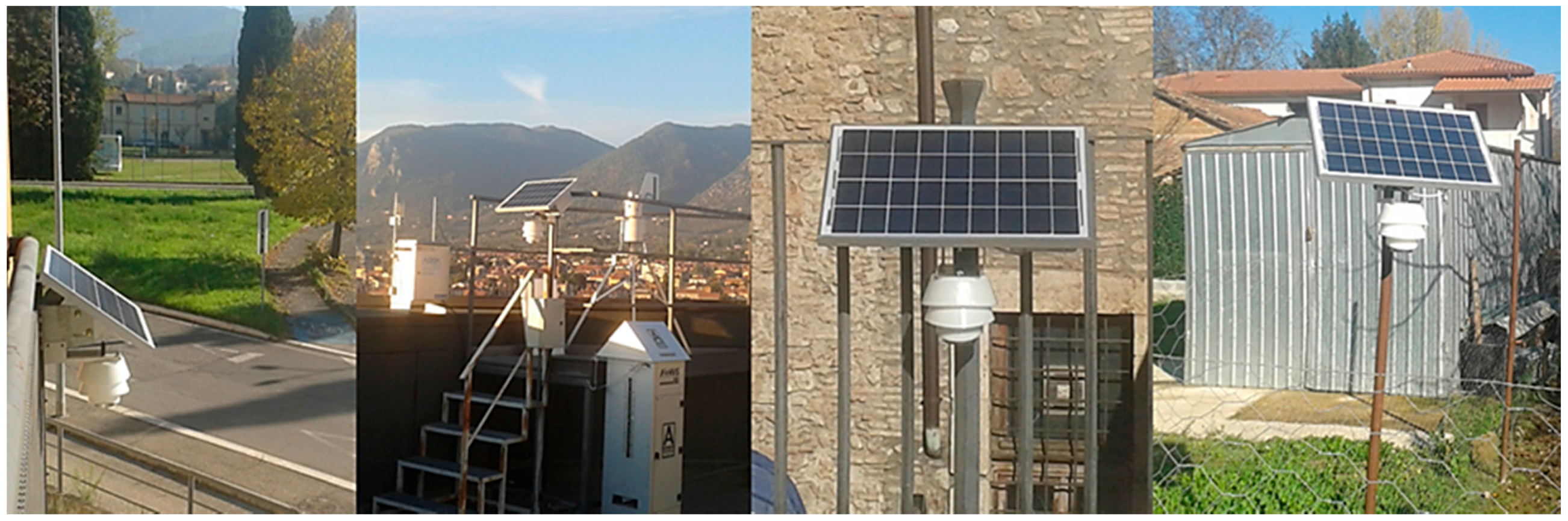
2.1. Sampling Sites and Sampling Equipment

The first phase of this study required great commitment and large amount of time for the identification and the choice of the best locations for the installation of 23 samplers. At first, in the selection of locations, a particulate matter dispersion grid, already developed by the regional agency for environmental protection (ARPA Umbria), was used as a reference system (Figure 1). It was also very important to guarantee that each sampler (SMART SAMPLER Fai Instruments, Fonte Nuova, Roma, Italy) was positioned at the same height (within 4 m) and with the same exposition (southern exposition) to ensure homogeneous sampling conditions. Particular attention was also paid to the representativeness of sites with respect to each local emission source of PM, as follows:

-

power plant for waste treatment located in the West of the city;

-

railway;

-

vehicular traffic due to the presence of streets with heavy traffic;

-

domestic biomass heating;

-

very extensive steel plant in the East of the city.

Table 1. Geographical coordinates of the monitoring sites of Terni.

Type of Site & Major Local PM Emission Sources		Geographical Coordinates
		Latitude	Longitude
RI	Industrial Site-Power Plant & Biomass Domestic Heating	42°33′52.02″ N	12°35′21.94″ E
MA	Industrial Site-Power Plant	42°33′41.42″ N	12°36′19.05″ E
FA	Industrial Site-Power Plant	42°33′03.19″ N	12°36′29.76″ E
GI	Industrial Site-Power Plant & Railway	42°34′06.28″ N	12°36′48.27″ E
FR	Industrial Site-Power Plant & Biomass Domestic Heating	42°33′53.22″ N	12°37′11.44″ E
CB	Industrial Site-Power Plant	42°33′20.30″ N	12°37′20.45″ E
PI	Urban Background Site (South of the City)	42°32′56.96″ N	12°37′52.26″ E
BR	Urban Background Site (North of the City)	42°34′56.19″ N	12°37′23.30″ E
AR	Urban Background Site (North of the City)	42°34′34.23″ N	12°37′39.88″ E
CR	Industrial Site-Power Plant & Railway	42°34′09.49″ N	12°37′39.81″ E
HG	Urban Site-Vehicular Traffic & Railway	42°34′19.32″ N	12°37′56.02″ E
SA	Urban Site-Heavy Vehicular Traffic	42°33′45.16″ N	12°38′18.45″ E
PV	Urban Site-Vehicular Traffic	42°33′06.96″ N	12°38′35.20″ E
LG	Urban Background Site (South of the City)	42°32′59.75″ N	12°39′01.16″ E
CZ	Urban Site-Vehicular Traffic	42°34′06.90″ N	12°38′52.97″ E
HV	Urban Site-Vehicular Traffic	42°33′58.33″ N	12°39′04.74″ E
UC	Urban Site-Vehicular Traffic	42°33′38.09″ N	12°38′47.62″ E
CA	Urban Site-Heavy Vehicular Traffic	42°33′39.01″ N	12°39′03.11″ E
CO	Industrial Site-Steel Plant & Heavy Vehicular Traffic	42°33′34.23″ N	12°39′22.62″ E
RO	Industrial Site-Steel Plant	42°33′51.16″ N	12°39′39.15″ E
OB	Industrial Site-Steel Plant	42°34′18.64″ N	12°40′05.57″ E
PR	Industrial Site-Steel Plant	42°34′20.30″ N	12°40′44.23″ E
CP	Industrial Site-Steel Plant	42°33′31.65″ N	12°40′36.04″ E

reports the geographical coordinates of the 23 selected sites. BR, AR (North of the city), PI and LG (South of the city) are sites located just outside the high density urban areas (urban background sites); MA, RI, GI, FR, CR, HG, FA and CB are situated in the West of the city, in an industrial area near the power plant for waste treatment (Terni En.A.) where domestic biomass heating systems are used; RO, PR, OB and CP are industrial sites close to (RO and PR) and in proximity (OB and CP) of the steel plant, in the East of the city (Terni AST); CO is a site located between the steel plant and the city center; CZ, HV, SA, UC, CA and PV are sites situated in high density urban areas and/or near heavy traffic streets (urban sites). In these 23 selected sites, innovative smart samplers (Figure 2) that have never been used on field before were installed.

Smart samplers are low cost, small, light, automatic, self-powered (with a power supply system constituted by a rechargeable battery and a small solar panel) and characterized by a flow of 0.5 L/min (with a consumption of 0.2 W for the intake system). The use of these samplers, which can be installed on balconies, railings, or light poles, improved access to a larger number of sampling locations, consenting to design an inexpensive, extended and extensive network across Terni. Hence, thanks to the utilization of the smart samplers, it was possible to obtain analytical data of the PM elemental components with a monthly time resolution (good representativeness) and at the same time with a huge spatial resolution (approximately 1 km of distance between the samplers) that could not be obtained by using the conventional 24 h samplers. Furthermore, due to the capacity of such samplers to work autonomously for long periods of time, the monitoring campaign had substantial reduction of associated costs. Smart samplers that possess a size selection inlet (PM₁₀ or PM_2.5) protected from the sun and rain by a small shield were equipped with PM₁₀ sampling head filter system (filter holder diameter 37 mm). Samples of PM₁₀ were collected by using Teflon membrane filters (PTFE membranes, 37 mm diameter, 2 μm pore size, PALL Corporation, Port Washington, New York, NY, USA). All the membrane filters were weighed before and after the sampling, in order to gravimetrically determine the PM₁₀ mass concentration. Smart samplers are equipped with a SD card from which it was possible to download the volumes of sampled air (m³), used for the calculation of the mass concentration of PM₁₀ and its elemental components. The monitoring campaign was carried out from December 2016 to April 2017. The lack of PM₁₀ mass concentration values and elemental concentration values for some collection sites is due to the progressive extension of the monitoring network during the monitoring campaign and sometimes to the malfunction of some samplers. Therefore, it was not possible to acquire sampling data with monthly time resolution at each of the 23 collection sites.

2.2. Analytical Procedure

The analytical procedure for the elemental chemical fractionation, previously optimized and validated [14,15,16], was carried on each PTFE membrane collected during the campaign. This procedure allows to discriminate water-soluble from insoluble fraction of each analyzed element and resulted to be useful in increasing the selectivity of each element as source tracer [14]. First, the supporting polymethylpentene rings were removed from each sampled PTFE membrane. During the first phase of the chemical fractionation procedure, the sampled PTFE membranes were extracted in an ultrasonic bath in 10 mL of deionized water (produced by Arioso UP 900 Integrate Water Purification System) for 30 min. The extracted solutions were then filtered on a cellulose nitrate filter (0.45 μm pore size, Merck Millipore Ltd., Billerica, MA, USA). After the extraction step, both the cellulose nitrate filter and the original PTFE filter were acid-digested in a microwave oven (Ethos Touch Control with Q20 rotor, Milestone, Italy) by using 2 mL of HNO₃ (67% Promochem) and 1 mL of H₂O₂ (30% Suprapur, Merck Millipore Ltd., Billerica, MA, USA). In the beginning of the digestion program, the temperature was linearly increased to 100 °C in 5 min. In the second step, the temperature was linearly increased to 180 °C in 12 min. In the third step, the temperature was kept at 180 °C for 15 min. After 30 min of ventilation and cooling down, the digested solutions were diluted in 50 mL of deionized water. These solutions were filtered with syringe filters (25 mm diameter, 0.45 μm pore size, GVS Filter Technology, Morecambe, UK). The concentrations of 34 elements (Al, As, B, Ba, Bi, Ca, Cd, Ce, Co, Cr, Cs, Cu, Fe, Ga, La, Li, Mg, Mn, Mo, Na, Nb, Ni, Pb, Rb, Sb, Sn, Sr, Ti, Tl, U, V, W, Zn and Zr) were determined in both extract and mineralized residue fractions obtained from each sample by using inductively coupled plasma mass spectrometry (ICP-MS, Bruker 820-MS, Billerica, MA, USA).

2.3. Statistical Analysis

Multivariate statistical computations were performed by the statistical software: R-3.0Gui (32-bit) for Windows (R-project for statistical computing). Multivariate analyses were operated on the data yielded by the analytical determinations on the elemental components of PM₁₀ at each collection site. Two principal component analyses (PCA) were performed. The first one was performed for the 23 monitoring sites by including the averages of the 34 monthly total elemental concentration data (sum of the extracted and residual fractions) recorded at each collection site. The second one was performed for the 23 monitoring sites by including the 34 total elemental concentration data (sum of the extracted and residual fractions) recorded each month at each collection site. The first PCA was performed to separate or group the monitoring sites depending on the type and on the concentration of the source tracers recorded at each site in order to identify the main emission source tracers and their action at each site. The second PCA was performed in order to assess the monthly action of the source tracers at each site and to evaluate the monthly variations of the elemental components of PM₁₀ in the monitored area. The 23 monitoring sites benefit from the choice of the best locations for the 23 smart samplers, hence collection sites are well differentiated for type and location, allowing a detailed discussion about differences in source nature and monthly contributions. In the data set used, some outliers (six outliers in Cr, Fe and Ni water-soluble fraction concentrations of two samples collected in December 2016 at FA and at CA, reasonably attributed to the contamination of these samples during the sample preparation for the extraction procedure) were excluded after having assessed that their presence increased unstable results of PCA.

2.4. Element Solubility Percentages

Solubility percentages of PM₁₀ elemental components were calculated by dividing the soluble fraction of each element analyzed to its total fraction (sum of the extracted and residual fractions) and multiplying by 100. The monthly solubility percentage for each element analyzed in the entire monitored area was obtained making each month an average of the solubility percentages calculated for each element at all the 23 monitoring sites. Standard deviations were calculated to evaluate the contribution of local emission sources to the variability of the elements solubility in the entire monitored area.

3. Results and Discussion

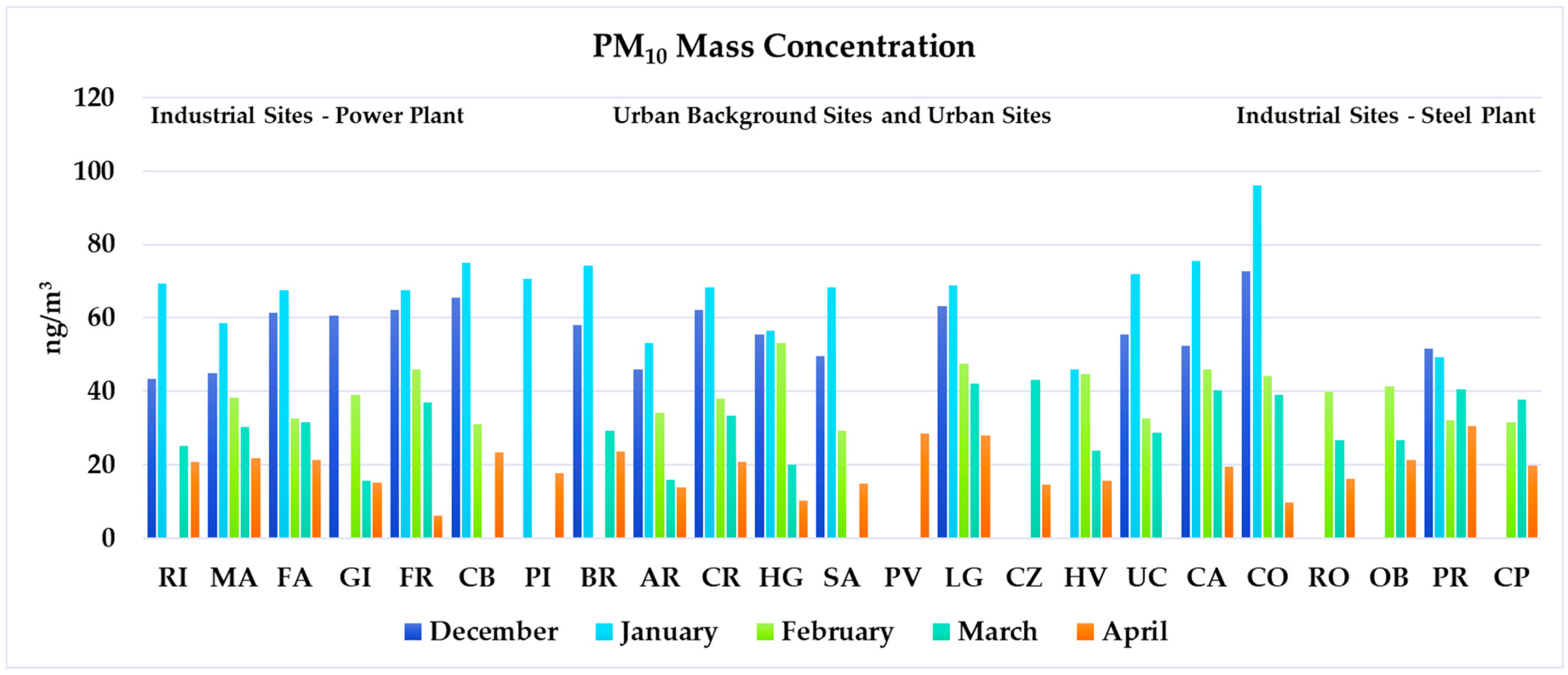
3.1. PM₁₀ Mass Concentration

Figure 3 reports the mass concentrations of PM₁₀ recorded in the 23 collection sites during the five-month monitoring campaign. The left and the right sector of the graphs in Figure 3 and Figure 4 represent, respectively, the data obtained by the collection sites located in the West (industrial sites near the power plant) and in the East (industrial sites in proximity or close to the steel plant) of the city. The central part of the graphs represents the urban sites PV, CZ, HV, SA, UC and CA.

The average of PM₁₀ mass concentrations recorded at all the collection sites of Terni during the monitoring campaign resulted of 42.3 μg/m³ (56.5 μg/m³ in December, 66.9 μg/m³ in January, 39 μg/m³ in February, 30.7 μg/m³ in March and 18.3 μg/m³ in April). The data above demonstrate that a clear increase in PM concentration occurred in all the sites during the winter. The highest PM₁₀ mass concentration (96 μg/m³) was recorded in January, during the colder period, at CO located between the heavily trafficked streets of the city and the steel plant. The lowest PM₁₀ mass concentration (6.2 μg/m³) was recorded in April, during the warmer period, at the monitoring station FR located in the West of the city in an industrial area near the power plant, far from the city center. The data in Figure 3 show that the concentration of PM₁₀ was driven by the contribution of different PM local emission sources as well as by the meteorological conditions. In general, the PM₁₀ mass concentration reflects the strength of the contribution from traffic-related sources at these sites [14]. In fact the highest values of PM₁₀ were recorded during the winter at urban sites CO, CA and UC. The increase of PM₁₀ mass concentrations during the colder months (December and January) can be explained by a combination of two factors: the less efficient mixing of the lower atmosphere during the winter and the strength of some seasonal PM sources, which include domestic heating [18,19,21]. The meteorological conditions of Terni basin limit the dispersion and enhance the accumulation of the atmospheric pollutants. Therefore the local circulation is often weak and this leads to a more stable atmosphere which is generally responsible for a concentration increase in all PM chemical species. Particularly during the winter, the meteorological conditions favor the development of temperature inversions, leading to extended periods of high atmospheric stability.

3.2. Elemental Concentration

Spatially resolved data obtained by sampling in parallel at 23 collection sites consented to properly evaluate the spatial variability of PM₁₀ as well as of some PM₁₀ chemical components and in particular of tracers of the principal local sources. For example Figure 4 reports the monthly values of the total concentrations (sum of the extracted and residual fractions) of Ni, Cu and Rb in PM₁₀ collected from the 23 collection sites during the five-month monitoring campaign. Figure 4 shows how, also for the elements, the highest elemental concentrations, at all the 23 monitoring sites, were recorded during the colder months, due to the presence of additional PM sources and/or to the lower mixing of the atmosphere [18]. The concentration of most elements increased with the level of urbanization at the collection site and with the proximity of the site to one of the main emission sources of the city: the steel plant.

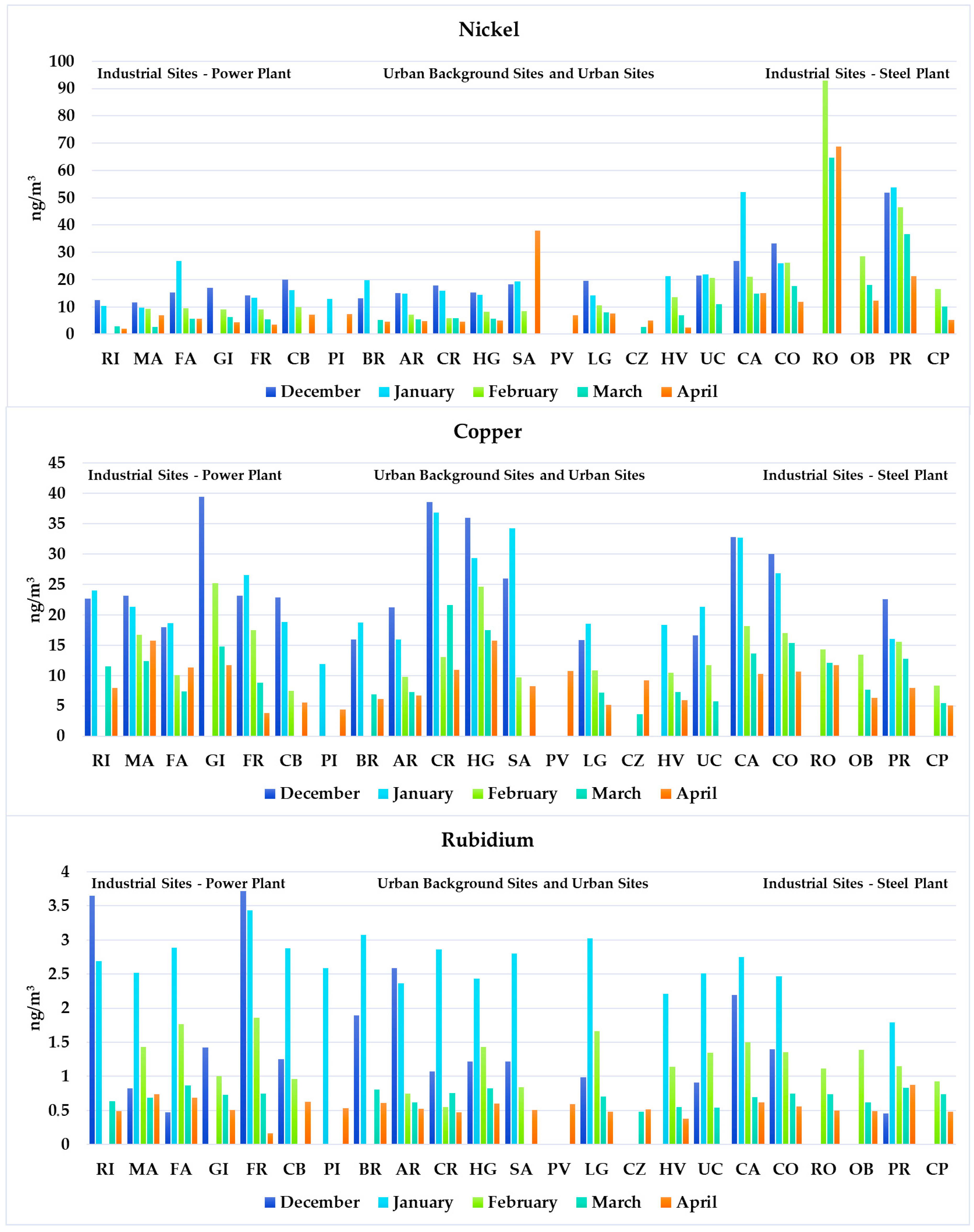
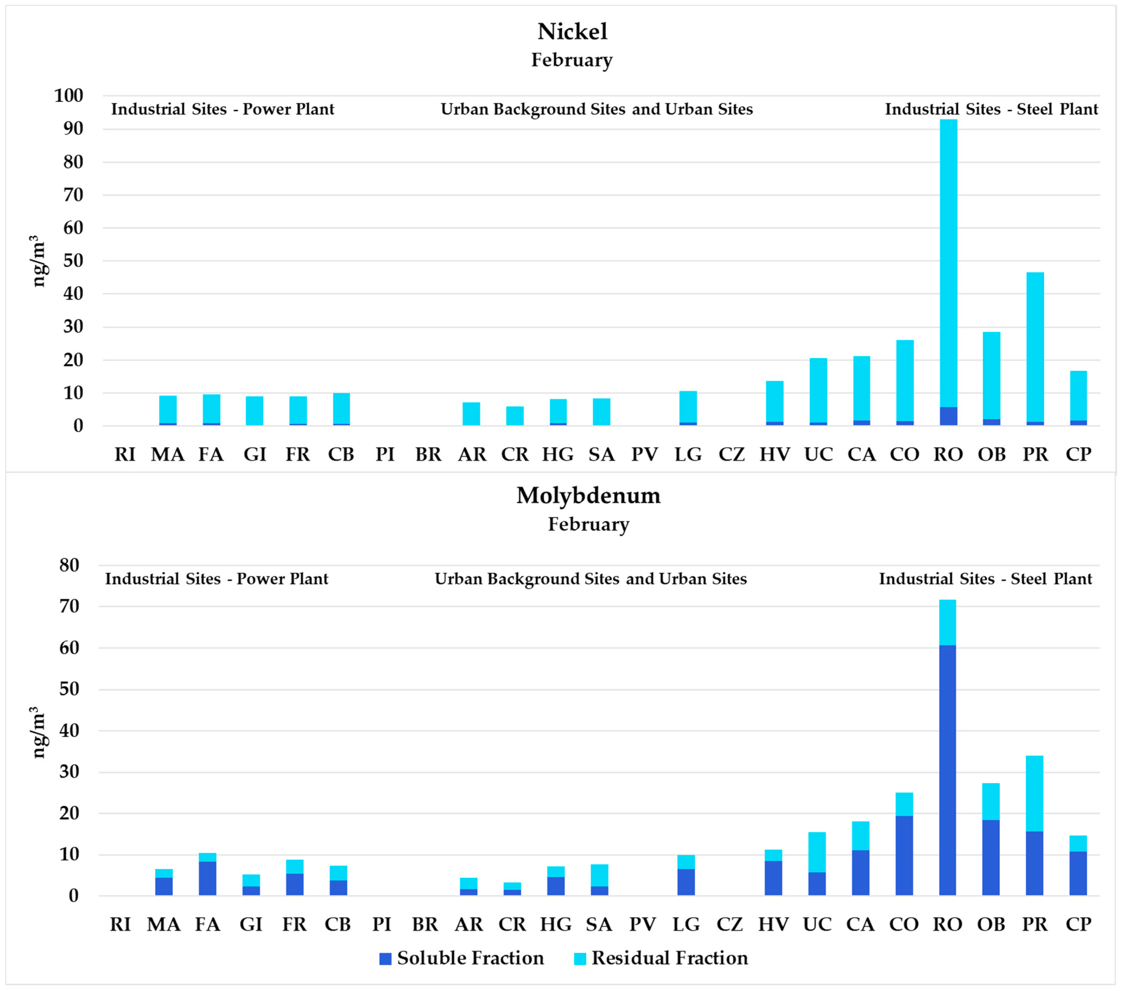
3.2.1. Ni, Cr, Mn, Mo, Pb and Fe Concentration

Cr, Mn and Mo showed the same behavior as Ni (upper panel of Figure 4) with a relevant increase of concentrations at the sites in proximity of the steel plant: RO, PR, OB, CP and CO. The highest concentrations of Ni were individuated in February at RO: 93 ng/m³. It is worth noting that this value is almost five times higher than the European Union (EU) target value (20 ng/m³), calculated on yearly averages (EU 2008/50/CE). Ni, Cr, Mo and Mn were identified as the main source tracers of the steel plant emission source. Cr and Ni are the basic composition of stainless steel which allows them to be the known tracers of the industry. Cr enables the steel to become resistant to chemical oxidation. Ni functions to create properties such as strength, ductility and toughness. Mn and Mo are secondary components of the stainless steel. Mo increases the corrosion resistance of the steel. Mn is used to increase toughness and tensile strength [22]. Even though the general behavior of the four tracers was similar, the results showed that Ni and Mo resulted less dispersed than Cr and Mn. The limited dispersion of these elements in the monitored area suggests that particles containing Ni and Mo had a lower diffusion capacity than those containing Cr and Mn. The low spatial dispersion of this steel plant related contribute suggest that, at least in part, mechanical and abrasive processes are more relevant than combustion ones. In fact, it is well known that fine particles, mainly produced by combustive processes, are easily carried by the wind, while coarse ones, mainly produced by mechanical and abrasive processes, tend to remain within the local emission area [23]. Each emission source is responsible for the release of particles having different dimensional ranges and containing chemical species having different solubility. Figure 5 reports the concentration of Ni and Mo measured in their soluble and residual fractions during the month of February. It is possible to observe that the two elements showed quite the same dispersion profiles, but they had a very different solubility distribution: Mo was emitted mainly as soluble species, while Ni was almost entirely contained in the residual fraction. Hence, it is possible to suppose that the steel plant released course particles containing mainly water-soluble species of Mo and insoluble species of Ni. The concentration of Pb demonstrated a consistent distribution throughout the city. At site PR, close to the steel industry, the Pb concentrations were especially high. This suggests that Pb must be emitted by the steel plant, possibly when it is added to carbon-steels in order to improve their machinability. Fe concentration (mainly present in the insoluble fraction) is also affected by the contribution from the steel plant, but it showed a different spatial profile respect to Ni, Cr, Mo and Mn, which are to be considered as more selective steel plant source tracers [24]. Fe in fact is also influenced by vehicular traffic and railway emission sources. Concentration peaks of Fe (>1000 ng/m³) in PM₁₀ were individuated during the winter at CA which is in proximity of heavy traffic streets, at sites close to the steel plant (RO and PR) and at CO, which is located between the steel plant and the high density urban area and at sites in proximity of the railway (GI, CR and HG).

3.2.2. Cu and Sb Concentration

As it is possible to see from the second panel of Figure 4, Cu resulted to be a more representative traffic-related source tracer. It showed concentration peaks in December only at sites located in proximity of heavy traffic streets (CA, SA and CO) and at sites in proximity of the railway (GI, CR and HG). Cu, Fe and Sb showed a similar distribution pattern at sites HG, CA and CO, in which their concentrations are relatively high because they are in proximity of the most trafficked roads of the city. Differently to what was previously described for the steel plant tracers, for Cu and Sb, the differences in terms of concentration between the monitoring sites resulted less marked, highlighting the role of vehicular traffic as the most common and distributed emission source of the city.

3.2.3. Rb, Bi, Sr, Mg and V Concentration

Finally, as it is possible to note from the third panel of Figure 4, Rb was emitted in higher concentrations during the winter months of December and January at sites in the West of the city (left part of the graph). Rb (main in the water-soluble fraction) was emitted in highest concentrations in December at sites RI and FR which are located in an industrial area in proximity of the power plant where domestic biomass heating systems are used. Therefore, Rb (water-soluble fraction) was identified as the most representative source tracer of biomass burning. It is worth noting that Rb concentration during the month of December also reflected the contribution of New Year’s fireworks, together with Bi, Sr and Mg. The analyses of the spatial variability in concentrations of other elements such as V did not reveal significant differences between the sites, without defining clear source profiles. The spatial homogeneity of V in the PM₁₀ within the city is due to the lack of influence of local sources responsible for its emission.

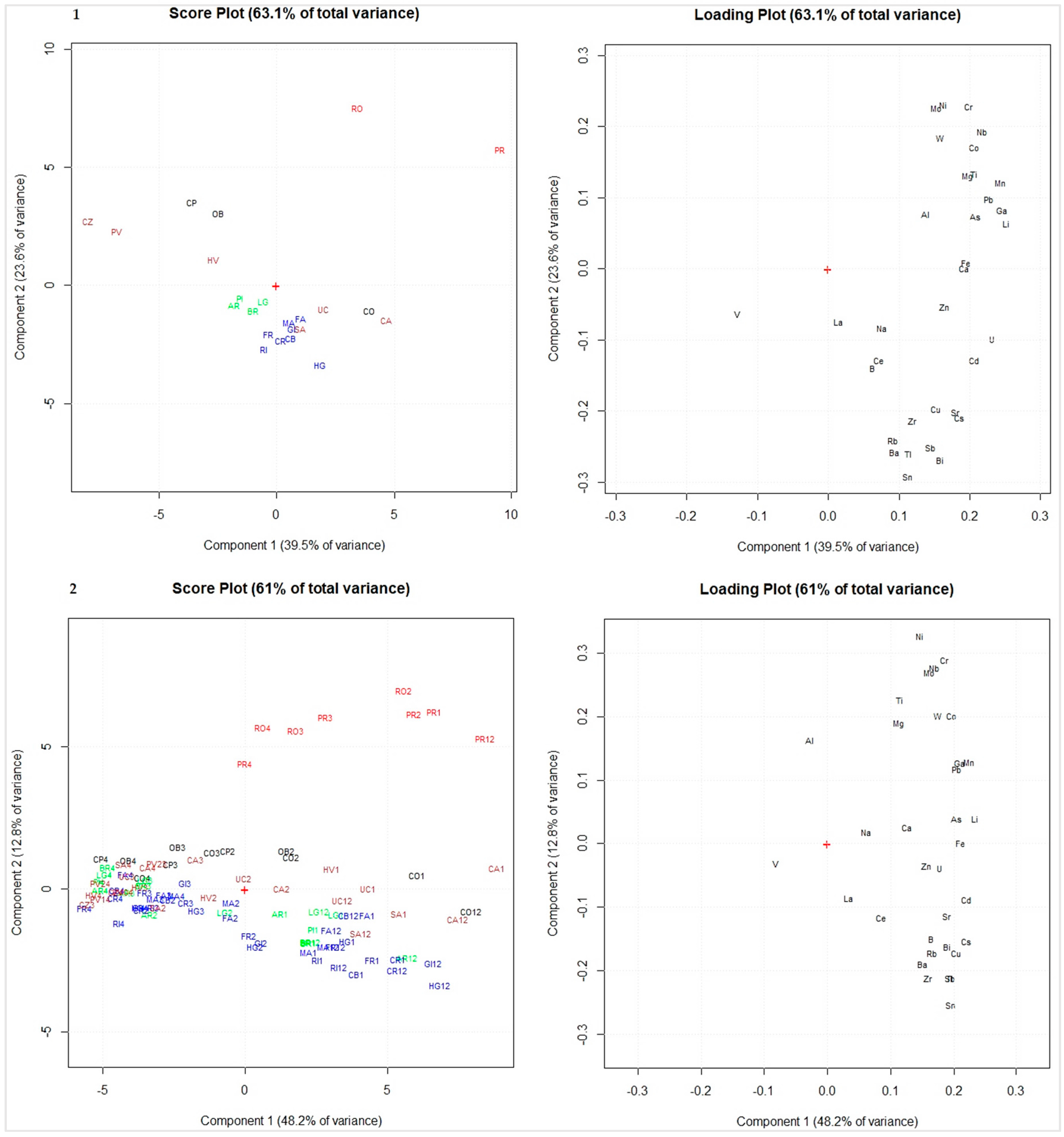
3.3. Source Tracers Identification by Principal Component Analysis

Results from the two principal component analyses performed in this study were evaluated and reported in Figure 6; all the total concentrations of the elemental components of PM₁₀ recorded were considered to identify the source tracers. The monitoring sites were represented in the left panels of Figure 6 with different colors depending on the type and location of each site, as follows:

-

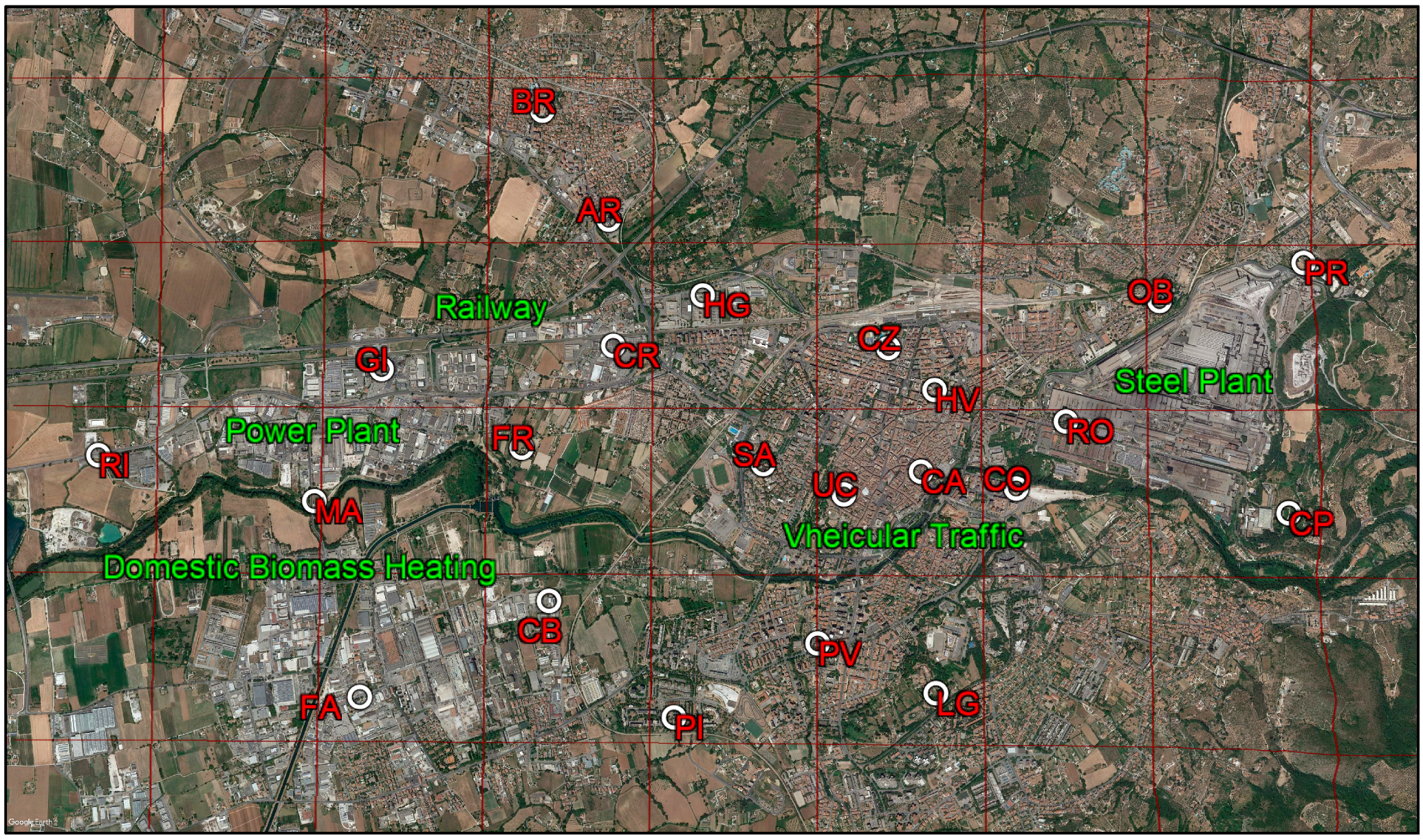
the urban background sites, located in the South and in the North of the city, outside the high density urban areas, (BR, AR, PI and LG) are represented with the green color;

-

the sites situated in the West of the city, in the industrial area near the power plant for waste treatment where domestic biomass heating systems are used (MA, RI, GI, FR, CR, HG, FA and CB) are represented with the blue color;

-

the sites located in the East of the city, in proximity of the steel plant (OB and CP) or between the steel plant and the city center (CO) are represented with the black color;

-

the sites located in the East of the city, close to the steel plant (RO and PR) are represented with the red color;

-

the urban sites, situated in high density urban areas and/or near heavy traffic streets (CZ, HV, SA, UC, CA and PV) are represented with the brown color.

An overview of all sources affecting the 23 monitoring sites used for the multivariate statistical analysis was obtained by performing a first preliminary PCA (upper panels of Figure 6) including the averages of all the 34 monthly total elemental concentration data (sum of the extracted and residual fractions) recorded at each collection site. Thanks to the first PCA, it was possible to separate or group the monitoring sites (scores) in the score plot depending on the type and on the concentration of the source tracers (loading) recorded at each site (upper panels of Figure 6). Hence, it was possible to properly identify the main source tracers (loadings) of the monitored area and their action at each site. The 63.1% of the total variance was explained by the first two principal components (PC1 and PC2). The urban background sites (green color) were positioned in the center of the score plot (left upper panel of Figure 6) because at these monitoring sites, lower concentrations of all the elemental components of PM₁₀ were recorded. The sites in the industrial area near the power plant (blue color), were separated from these on the PC2 by Zr, Sb, Bi, Tl, Sn, Ba and Rb, which were classified as biomass burning source tracers. The urban sites (brown color) resulted well distributed on the two principal components confirming the role of vehicular traffic as most common and distributed emission source of the city. The sites CZ, PV and HV, which are located in the city center but quite distant from the heavy traffic streets, were separated from UC, SA and CA by Sb, Cd, Fe, Cu, Ba and Zn, which are typical source tracers of vehicular traffic, by Rb, tracer of domestic heating and by Bi and Sr, which are fireworks burning source tracers. The sites at the East of the city, closer to the steel plant, were separated from all the other monitoring sites on the PC2 by Ni, Cr, Mo and Mn, which were already identified as steel plant source tracers, and by Ti, Nb, W, Co, Mg and Pb. It is interesting to note that PR was separated from RO on the PC1 by Pb, Mg, Mn and Ti. This suggests the presence of different steel plant local emission sources. The sites in proximity of the steel plant or between the steel plant and the city center (black color) were positioned exactly between the urban sites and the sites closer to the steel plant, confirming the action of both vehicular traffic and steel plant emission source at site CO. V did not reveal significant differences between the sites confirming the spatial homogeneity of V in the PM₁₀ within the city. From the second PCA performed, it was possible to assess the monthly action of the source tracers at each monitoring site and to evaluate the monthly variations of the elemental components of PM₁₀ at each collection site. As can be seen from the lower panels of Figure 6, the first two components explained the 60.6% of the total variance. The number associated to the name of the monitoring sites in the left lower panel of Figure 6 correspond to the month of sampling at each site: December: 12, January: 1, February: 2, March: 3 and April: 4. The second PCA confirmed the progressively decrease of PM₁₀ elemental components’ concentrations at each site from December to April, due to the presence of additional PM sources and/or to the lower mixing of the atmosphere during the colder months. The months of sampling at each collection site were separated on the PC1 from the right part to the left part of the score plot, following the monthly sequence of sampling, from December to April. The different types of monitoring sites were maintained separated on the PC2 confirming the efficiency of the source tracers identified from the first PCA performed.

3.4. Seasonal Variability of Element Solubility Percentages in PM₁₀

The monthly solubility percentages obtained for each element analyzed in the entire monitored area (

Table 2. Means (AM) and standard deviations (SD) of the elements solubility percentages (%) calculated monthly for each element at all the 23 monitoring sites.

Month	December			January			February			March			April
	AM	±	SD	AM	±	SD	AM	±	SD	AM	±	SD	AM	±	SD
Li	65	±	6	68	±	5	57	±	13	34	±	9	68	±	16
B	51	±	14	79	±	9	67	±	19	53	±	29	70	±	22
Na	39	±	17	44	±	27	53	±	10	55	±	15	49	±	11
Mg	51	±	6	57	±	10	47	±	9	37	±	6	54	±	9
Al	9	±	3	9	±	3	5	±	2	1	±	1	3	±	1
Ca	47	±	17	64	±	13	50	±	15	26	±	11	57	±	15
Ti	1	±	0	3	±	2	4	±	2	1	±	0	4	±	2
V	32	±	14	51	±	27	51	±	25	45	±	18	75	±	11
Cr	6	±	2	6	±	3	4	±	2	3	±	2	9	±	4
Mn	45	±	5	47	±	5	38	±	9	26	±	9	45	±	8
Fe	3	±	2	3	±	2	3	±	2	1	±	0	4	±	1
Co	15	±	4	20	±	15	14	±	6	10	±	6	23	±	13
Ni	10	±	5	9	±	3	7	±	3	5	±	3	15	±	8
Cu	22	±	5	22	±	4	23	±	7	12	±	7	32	±	7
Zn	47	±	14	54	±	12	43	±	11	13	±	7	37	±	12
Ga	11	±	3	14	±	3	13	±	6	5	±	3	32	±	20
As	59	±	12	65	±	8	51	±	21	15	±	9	87	±	8
Rb	67	±	21	90	±	1	86	±	8	52	±	7	70	±	14
Sr	48	±	12	74	±	10	65	±	16	45	±	11	75	±	10
Zr	1	±	1	1	±	1	5	±	3	1	±	1	6	±	7
Nb	1	±	1	1	±	1	4	±	2	1	±	1	39	±	21
Mo	43	±	7	60	±	10	60	±	16	63	±	9	82	±	7
Cd	89	±	9	70	±	13	71	±	18	38	±	20	93	±	5
Sn	1	±	0	2	±	1	7	±	4	4	±	2	15	±	6
Sb	26	±	5	35	±	9	27	±	12	29	±	10	53	±	12
Cs	77	±	4	81	±	2	66	±	9	31	±	7	95	±	5
Ba	29	±	9	42	±	10	28	±	0	28	±	0	47	±	15
La	7	±	4	8	±	6	12	±	8	3	±	2	6	±	4
Ce	4	±	2	4	±	3	11	±	8	3	±	1	3	±	5
W	37	±	6	47	±	6	42	±	13	43	±	15	70	±	20
Tl	81	±	5	77	±	5	69	±	13	49	±	10	95	±	20
Pb	19	±	4	12	±	3	15	±	5	6	±	4	20	±	6
Bi	3	±	1	6	±	1	8	±	4	5	±	3	28	±	29
U	11	±	2	7	±	4	15	±	7	9	±	6	88	±	0

) allowed to evaluate the seasonal variability of the element soluble fractions in PM₁₀ and to estimate the environmental mobility and the bio-accessibility of each element [18]. From the standard deviations calculated, it was also possible to evaluate the contribution of local sources to the variability of the elements solubility in the entire monitored area. Cd, B, Rb, Sr, Mo, Cs and Tl showed the highest solubility percentages and bio-accessibility during the five-month monitoring campaign while Al, Ti, Cr, Fe, Ni, Zr, Nb, Sn, La, Ce, Pb and Bi resulted released mostly in the residual fraction.

Zn, Ni, Fe, Cr and Pb are considered as some of the most potential dangerous elements for human health. However, the bio-accessibility of these elements in the monitored area appeared quite limited because they resulted predominantly present in the residual fraction at all the 23 locations. The solubility percentages of the elements in PM₁₀ did not show a clear seasonal variability. From December to March, the elements solubility percentages resulted constant, while a slight, and in some cases considerable, increase was recorded for the majority of the elements in the month of April. This increase might be due to the variation of some local emission sources that released particles containing mostly insoluble chemical species.

4. Conclusions

The results obtained proved the efficiency of the new experimental procedure elaborated for the evaluation of the spatial variability of PM₁₀ and its chemical components through the acquisition of spatially resolved data. In particular, the innovative smart samplers, used for the first time in this campaign, allowed to build an extended and extensive monitoring network, with low associated costs, which was able to represent the different emission source contributes to total PM₁₀ in the monitored area. From the acquisition of spatially resolved data, it was possible to properly evaluate the dispersion capacity of PM₁₀ and its elemental components. The elemental analyses associated with the chemical fractionation procedure and the statistical treatment of the data allowed to identify the source tracers of each PM₁₀ local emission source which will be used for future source apportionment studies. Chemical fractionation, by providing information on the chemical form, improved the selectivity of different source tracers. Spatial variability of Ni, Cr, Mn (insoluble fraction) and Mo (water-soluble fraction) concentrations showed the steel plant role in the emission of PM₁₀. Spatial variability of Fe (insoluble fraction) resulted to be correlated not only to the steel plant emission but also to the influence of vehicular traffic sources. The role of this emission source was also confirmed by the spatial variability of element such as Sb and Cu, which showed high concentrations at the sites near high-traffic streets and the railway. Rb (soluble fraction) was confirmed to be a good tracer of biomass combustion processes. This experimental approach, based on the acquisition of spatially resolved data for analyzing spatial variability of PM₁₀ and its chemical components, will be effective for the validation of dispersion models without the high costs associated to an air quality monitoring network.

References

1. Pope, C.A.; Burnett, R.T.; Thun, M.J.; Calle, E.E.; Krewski, D.; Ito, K.; Thurston, G.D. Lung Cancer Cardiopulmonary Mortality, and Long-term Exposure to Fine Particulate Air Pollution. J. Am. Med. Assoc. 2002, 287, 1132–1141. [Google Scholar] [CrossRef]
2. Hwang, I.; Hopke, P.K. Estimation of Source Apportionment and Potential Source Locations of PM2.5 at a West Coastal IMPROVE Site. Atmos. Environ. 2007, 4, 506–518. [Google Scholar] [CrossRef]
3. Conti, G.O.; Heibati, B.; Kloog, I.; Fiore, M.; Ferrante, M. A review of AirQ Models and their applications for forecasting the air pollution health outcomes. Environ. Sci. Pollut. Res. 2017, 24, 6426–6445. [Google Scholar] [CrossRef] [PubMed]
4. Vitali, L.; Morabito, A.; Adani, M.; Assennato, G.; Ciancarella, L.; Cremona, G.; Giua, R.; Pastore, T.; Piersanti, A.; Righini, G.; et al. A Lagrangian modelling approach to assess the representativeness area of an industrial air quality monitoring station. Atmos. Pollut. Res. 2016, 7, 990–1003. [Google Scholar] [CrossRef]
5. Weil, J.C.; Sykes, R.I.; Venkatram, A. Evaluating air quality models: Review and Outlook. J. Appl. Meteorol. 1992, 31, 1121–1145. [Google Scholar] [CrossRef]
6. Irwin, J.C. A suggested method for dispersion model evaluation. J. Air Waste Manag. Assoc. 2014, 4, 255–264. [Google Scholar] [CrossRef]
7. Padoan, E.; Malandrino, M.; Giacomino, A.; Grosa, M.M.; Lollobrigida, F.; Martini, S.; Abollino, O. Spatial distribution and potential sources of trace elements in PM10 monitored in urban and rural sites of Piedmont Region. Chemosphere 2016, 145, 495–507. [Google Scholar] [CrossRef] [PubMed]
8. Kim, B.U.; Bae, C.; Kim, H.C.; Kim, E.; Kim, S. Spatially and chemically resolved source apportionment analysis: Case study of high particulate matter event. Atmos. Environ. 2017, 162, 55–70. [Google Scholar] [CrossRef]
9. Fox, D.G. Uncertainty in Air Quality Modeling. Bull. Am. Meteorol. Soc. 1984, 65, 27–36. [Google Scholar] [CrossRef]
10. Almeida, S.M.; Pio, C.A.; Freitas, M.C.; Reis, M.A.; Trancoso, M.A. Source apportionment of atmospheric urban aerosol based on weekdays/weekend variability: Evaluation of road re-suspended dust contribution. Atmos. Environ. 2006, 40, 2058–2067. [Google Scholar] [CrossRef]
11. Perrino, C.; Canepari, S.; Pappalardo, S.; Marconi, E. Time-resolved measurements of water-soluble ions and elements in atmospheric particulate matter for the characterization of local and long-range transport events. Chemosphere 2010, 80, 1291–1300. [Google Scholar] [CrossRef] [PubMed]
12. Moroni, B.; Ferrero, L.; Crocchianti, S.; Cappelletti, D. Aerosol dynamics upon Terni basin (Central Italy): Results of integrated vertical profile measurements and electron microscopy analysis. Rendiconti Lincei 2013, 24, 319–328. [Google Scholar] [CrossRef]
13. Guerrini, R. Qualità dell’aria nella provincia di Terni tra il 2002 e il 2011. Quad. ARPA Umbria 2012, XXXIII, 81–87. [Google Scholar] [CrossRef]
14. Canepari, S.; Pietrodangelo, A.; Perrino, C.; Astolfi, M.L.; Marzo, M.L. Enhancement of source traceability of atmospheric PM by elemental chemical fractionation. Atmos. Environ. 2009, 43, 4754–4765. [Google Scholar] [CrossRef]
15. Canepari, S.; Cardarelli, E.; Giuliano, A.; Pietrodangelo, A. Determination of metals, metalloids and non-volatile ions in airborne particulate matter by a new two-step sequential leaching procedure Part A: Experimental design and optimization. Talanta 2006, 69, 581–587. [Google Scholar] [CrossRef] [PubMed]
16. Canepari, S.; Cardarelli, E.; Giuliano, A.; Strincone, M. Determination of metals, metalloids and non-volatile ions in airborne particulate matter by a new two-step sequential leaching procedure Part B: Validation on equivalent real samples. Talanta 2006, 69, 588–595. [Google Scholar] [CrossRef] [PubMed]
17. Templeton, D.M.; Ariese, F.; Cornelis, R.; Danielsson, L.G.; Muntau, H.; Van Leeuwen, H.P.; Lobinski, R. Guidelines for terms related to chemical speciation and fractionation of elements. Definitions, structural aspects, and methodological approaches (IUPAC Recommendations 2000). Pure Appl. Chem. 2000, 72, 1453–1470. [Google Scholar] [CrossRef]
18. Canepari, S.; Astolfi, M.L.; Farao, C.; Maretto, M.; Frasca, D.; Marcoccia, M.; Perrino, C. Seasonal variations in the chemical composition of particulate matter: A case study in the Po Valley. Part II: Concentration and solubility of micro- and trace-elements. Environ. Sci. Pollut. R. 2014, 21, 4010–4022. [Google Scholar] [CrossRef] [PubMed]
19. Perrino, C.; Catrambone, M.; Dalla Torre, S.; Rantica, E.; Sargolini, T.; Canepari, S. Seasonal variations in the chemical composition of particulate matter: A case study in the Po Valley. Part I: Macro-components and mass closure. Environ. Sci. Pollut. Res. 2014, 21, 3999–4009. [Google Scholar] [CrossRef] [PubMed]
20. Harrison, R.M.; Yin, J. Particulate matter in the atmosphere: Which particle properties are important for its effects on health? Sci. Total Environ. 2000, 249, 85–101. [Google Scholar] [CrossRef]
21. Perrino, C.; Tofful, L.; Canepari, S. Chemical characterization of indoor and outdoor fine particulate matter in an occupied apartment in Rome, Italy. Indoor Air 2016, 26, 558–570. [Google Scholar] [CrossRef] [PubMed]
22. Blair, M.; Stevens, T.L. Steel Castings Handbook, 6th ed.; Steel Founders’ Society and ASM International: Novelty, OH, USA, 1995; pp. 2–34. [Google Scholar]
23. Li, R.; Wiedinmyer, C.; Hannigan, M.P. Contrast and correlations between coarse and fine particulate matter in the United States. Sci. Total Environ. 2013, 456–457, 346–358. [Google Scholar] [CrossRef] [PubMed]
24. Taiwo, A.M.; Harrison, R.M.; Shi, Z. A review of receptor modelling of industrially emitted particulate matter. Atmos. Environ. 2014, 97, 109–120. [Google Scholar] [CrossRef]
Figure 1. Map of monitoring sites of Terni (Google Earth Pro) with the particulate matter dispersion grid and the main local emission sources represented.
Atmosphere 08 00200 g001
Figure 2. Smart samplers (SMART SAMPLER Fai Instruments, Fonte Nuova, Roma, Italy) installed in 4 of the 23 monitoring sites of Terni.
Atmosphere 08 00200 g002
Figure 3. PM10 mass concentrations (μg/m3) recorded at the 23 collection sites during the five-month monitoring campaign.
Atmosphere 08 00200 g003
Figure 4. Variations of Ni, Cu and Rb monthly concentrations (ng/m3) recorded during the five-month monitoring campaign at the 23 collection sites.
Atmosphere 08 00200 g004
Figure 5. Soluble and residual fractions of Ni and Mo concentrations (ng/m3) recorded in February at the 23 collection sites.
Atmosphere 08 00200 g005
Figure 6. Panel 1—Score and loading plots of the PCA performed by using the averages of the 34 monthly total elemental concentration data recorded at each collection site. Panel 2—Score and loading plot of the PCA performed by using the 34 total elemental concentration data recorded each month at each collection site.
Atmosphere 08 00200 g006