Article

Synoptic Conditions Generating Heat Waves and Warm Spells in Romania

by
Lucian Sfîcă
1,
Adina-Eliza Croitoru
2,*,
Iulian Iordache
3 and
Antoniu-Flavius Ciupertea
4
1
Geography Department, Faculty of Geography and Geology, Alexandru Ioan Cuza University, Iași 700506, Romania
2
Department of Physical and Technical Geography, Faculty of Geography, Babes-Bolyai University, Cluj-Napoca 400006, Romania
3
Doctoral School, Faculty of Geography and Geology, Alexandru Ioan Cuza University, Iași 700506, Romania
4
Doctoral School, Faculty of Geography, Babes-Bolyai University, Cluj-Napoca 400006, Romania
*
Author to whom correspondence should be addressed.
Atmosphere 2017, 8(3), 50; https://doi.org/10.3390/atmos8030050
Submission received: 25 December 2016 / Revised: 15 February 2017 / Accepted: 24 February 2017 / Published: 1 March 2017
(This article belongs to the Special Issue Temperature Extremes and Heat/Cold Waves)

Abstract

:
Heat waves and warm spells are extreme meteorological events that generate a significant number of casualties in temperate regions, as well as outside of temperate regions. For the purpose of this paper, heat waves and warm spells were identified based on daily maximum temperatures recorded at 27 weather stations located in Romania over a 55-year period (1961–2015). The intensity threshold was the 90th percentile, and the length of an event was of minimum three consecutive days. We analyzed 111 heat wave and warm spell events totaling 423 days. The classification of synoptic conditions was based on daily reanalysis at three geopotential levels and on the online version of a backward trajectories model. The main findings are that there are two major types of genetic conditions. These were identified as: (i) radiative heat waves and warm spells (type A) generated by warming the air mass due to high amounts of radiation which was found dominant in warm season; and (ii) advective heat waves and warm spells (type B) generated mainly by warm air mass advection which prevails in winter and transition seasons. These major types consist of two and three sub-types, respectively. The results could become a useful tool for weather forecasters in order to better predict the occurrence of heat waves and warm spells.

1. Introduction

Extreme high temperatures and related events such as heat waves (HWs) and warm spells (WSs) have been largely documented to show that they have increased in magnitude and frequency over the last few decades in most regions of the planet [1,2,3,4,5,6,7,8,9,10,11,12,13]. Usually, when a relative threshold is used to define extreme high temperature events over the year, HWs term is employed for summer, late spring, and early winter events (May–September), while WS term is frequently used for winter, late autumn, and early spring events (October–April). They have become a very important issue as they imply a significant threat to life and property in times of accelerated population growth and climate change [14].
It has been documented that they have direct consequences on society and the environment, as well as indirect adverse consequences affecting different domains such as agriculture, water resources, energy demand, regional economies and human health [15,16,17,18]. Studies on HWs and WSs developed over the last three decades focused on their physical features or on different types of impact they have, especially on human health, thermal and air quality conditions [19,20,21], or heat-related mortality and morbidity [22,23,24,25,26]. The August 2003 HW alone is considered as the worst natural disaster in Europe of the last 50 years, with an estimated death toll exceeding 30,000 people [14,27], followed by other similar events such as in July 2007 with great impact on Southeastern Europe and in July 2010 bringing a historical HW in Eastern Europe [28].
Reducing the impacts of future HWs requires addressing fundamental questions, such as whether HWs can be predicted, detected and whether their impacts can be mitigated [6]. Under these circumstances, investigations on the relationship between HWs and atmospheric circulation are of great importance for any region, as weather forecasting should improve and become more efficient in order to alert people and authorities. In addition, the adaptation to increased HWs and WSs conditions could be a challenge for public authorities in the most prone regions to choose the most appropriate measures.
A better understanding of the large scale connections is essential to improve the forecasts of HWs and WSs. A growing number of studies have looked at the mechanisms that contribute to the formation and prediction of such extreme warm events in many regions of the world [6,14,29,30,31,32,33,34,35,36,37,38]. Most of those studies revealed that HWs and WSs do not occur independently of circulation conditions, but their occurrence is favored by certain flow configurations while unlikely under other ones. The relationship between circulation and the occurrence of prolonged extreme events is thus an important component of a climate system [1]. Certainly, the synoptic behavior of cyclones and anticyclones is an important manifestation of how large scale circulation can interact with weather extremes [14]. In recent decades, the frequency of blocking systems over Europe or different regions in Europe has increasingly generated HWs [37,38,39], while the number of low pressure systems south of 55° N has decreased [40,41,42]. Some other papers have demonstrated that an increase in the stability of the atmospheric circulation may partly explain the more frequent extreme air temperatures in Europe. Kysely [43,44,45] found that, in summer, more stable circulation types contribute to the occurrence of more intense and longer HWs. Moreover, the occurrence of thermal anomalies was found to be connected with longer lasting high pressure blocking events in summer and spring [39,42,46]. Extremes on both ends of the temperature distribution are closely connected to atmospheric blocking. Surface temperatures can be impacted by atmospheric blocking via radiative forcing or advection [39].
Information on HWs and WSs for Romanian territory is available in some studies developed at global or regional scale, based on gridded or observation data. Few recent studies analyzing indices of extreme temperatures at global, regional or national scale, including those related to HWs and WSs, revealed significant increasing trends over the period 1951–2010 in Romania [13,36,47,48]. Some other studies focused on smaller areas such as Southern Romania or the Bârlad Plateau [49,50,51,52].
This paper will document the large-scale conditions associated with HWs and WSs occurrence in Romania as well as the analysis of anomalies associated with HWs and WSs in Romania. We presented a brief synoptic climatology of HWs and WSs identified for each circulation pattern. Such a multi-angle investigation of HWs and WSs has not been done so far in Romania. This subject is especially relevant for short and mid-term weather forecasting [36].

2. Experiments

2.1. Data Used

For this paper, HWs and WSs identification is based on daily maximum temperature (TX) data sets recorded in 27 weather stations across Romania over a 55-year period (1961–2015) (Figure 1).
The 55-year period (1961–2015) was chosen to avoid as much as possible inhomogeneities and gaps in the daily data that could be introduced by some non-climatic factors, such as changes in observational practices and timetables [53]. The recommendation of the World Meteorological Organization [54] is to maintain only those stations that have no more than 5% missing data. Finally, all the stations used for this study had no more than 0.5% missing daily data (Table 1).
Most data were freely downloaded from European Climate Assessment and Database project database (non-blend data) [55] and reconstructed from raw synoptic messages available on www.meteomanz.com. For four weather stations (Oradea, Timisoara, Targu Mures, and Brasov), the data sets were provided by the Romanian National Meteorological Administration (RNMA) [13]. For Romania, the temperature analysis for different types of HWs and WSs was performed based on gridded data of daily maximum temperature extracted from ROmanian ClimAtic DAtaset ROCADA datasets [56]. ROCADA is a new gridded dataset, containing national daily maximum and minimum temperatures covering 1961–2013 across Romania, and it was developed by the RNMA. It has a spatial resolution of 10 km and was based on 150 weather station measurements. Datasets are available on the World Data Center PANGAEA portal. We have used the ROCADA data base for mapping the composite mean of maximum temperature anomalies due to its better spatial resolution and accuracy compared to other gridded databases, such as E-OBS.
Synoptic analysis is based on maps for sea level pressure, air masses and fronts from the Daily Weather Bulletin of the RNMA for the interval 1961–2002 and from the Deutsche Wetterdienst for 2003–2015.
Meteorological input data for the trajectory simulations, the reanalysis datasets, freely provided by National Centers for Environmental Prediction (NCEP) and the National Center for Atmospheric Research (NCAR) Reanalysis were used. HYbrid Single-Particle Lagrangian Integrated Trajectory (HYSPLIT) application uses archived three-dimensional meteorological fields generated from observations and short-term forecasts [57]. In addition, for the description of weather conditions at continental level during HWs and WSs affecting Romania, composite maps were derived using the mean daily composites tool from Earth System Research Laboratory of National Oceanic and Atmospheric Administration (NOAA) [58].

2.2. Methods

2.2.1. HWs and WSs Analysis

There are no universal methods or criteria that can be used to classify extreme events globally or locally [59], including HWs. It is expected that more appropriate HWs definitions may emerge in the future [8]. At the same time as stated by [60], attention needs no longer to be restricted to a rigid definition of HWs, about which there is not necessarily any consensus. Most HWs definitions use two types of thresholds to identify events: thresholds for intensity (temperature) and thresholds for duration (days). For intensity, fixed or relative thresholds are usually employed [61].
HWs are defined as: (1) several-day periods with maximum or mean daily temperature above a specific threshold value [62,63,64]; (2) periods with apparent temperature (AT) above the 95th percentile which starts with a minimum 2.0 °C increase in relation to the preceding day [65]; and (3) periods longer than five consecutive days with TX exceeding at least 5 °C above the 1961–1990 daily TX norm [36,37,66]. In addition, there is no exact definition of HWs in terms of type of datasets used. Thus, many definitions could apply to HWs that quantify the duration and/or intensity of either nighttime minimum or daytime maximum temperatures as well as both of them or mean daily temperature [1,3,35,37,38,67,68]. Most papers referring to HWs use the aforementioned definitions, but some of them consider data sets only for a few months of the year (usually June–August or April–September). The intensity threshold can be defined as a fixed value (e.g., 30 °C or 35 °C) or a relative one (daily average, 90th or 95th percentile).
Since it is unusual to talk about heat events related to winter or late autumn/early spring, for this study we decided that it is more appropriate to use “heat waves” for the warm half of the year (April–September) and “warm spell” for the cold half of the year (October–March).
In this paper, the identification of HWs and WSs is based on the 90th percentile of daily maximum temperature as the intensity threshold, while the minimum length is of three consecutive days for each individual event. This is one of the most commonly used methods to identify HWs and WSs [69]. The daily percentile is calculated for each day of the year and then the TX of each day in the dataset is compared to the percentile value of the corresponding calendar day. The percentile was calculated for the baseline period 1981–2010 because according to WMO recommendations, for practical purposes, as weather forecasts, the baseline period should be the latest available: using a more recent period results in a slight improvement in predictive accuracy for elements that show a secular trend (that is, where the time series shows a consistent rise or fall in its values when measured over a long term) and would be viewed by many users as more “current” than 1961–1990 [54] and we consider that this would be more appropriate for the purpose of the study.
A similar reference period is already in use in climate forecast or in other recent climatic studies [28,36,70], mainly due to its higher relevance for the actual conditions of the climate. In addition, taking into account that our study aims to be used in weather forecast applied to climate conditions most people are familiar with—and not just to understand climate variability—it is recommended to use the last three decades as a reference period [71].
Later, when analyzing the synoptic conditions, we had to introduce a threshold for spatial coverage of the HWs and WSs. Thus, we considered only those HWs/WSs that were registered almost simultaneously over the greater part of Romania. When a HW/WS event of a minimum three consecutive days was identified in each weather station considered, but only two days are common for at least 75% of the weather station, we selected it as a HW/WS valid for this analysis. This approach was adopted due to the delay generated by air mass propagation: if in the South or in the East of the country a HWs/WSs strikes in day i and lasts until day i+2, in the opposite side of the country (North or West) it can begin on day i+1 and end in day i+3. Thus, in each area, the HW/WS lasts three days, but due to the delay introduced by air mass propagation, the common period with HW/WS conditions for the whole country is only two days (day i+1 and i+2). More specifically, we considered at least two out of three minimum consecutive days when the intensity threshold was simultaneously exceeded.
Under these conditions, we identified and analyzed 111 HW/WS events that hit simultaneously throughout Romania, cumulating 423 days.
In this paper, we focused our statistical analysis mainly on the number of days and not on the events number because in some multi-event seasons it is quite difficult to distinguish the separation between events. Some sources consider that a 20-day separation period is needed to consider a new HW or WS event [35]. Otherwise, it can be considered that later events can be caused by persistent overlying atmospheric conditions (i.e., event recurrence). This situation can generates bias in the overall count of HWs, while the total number of days would not be affected.

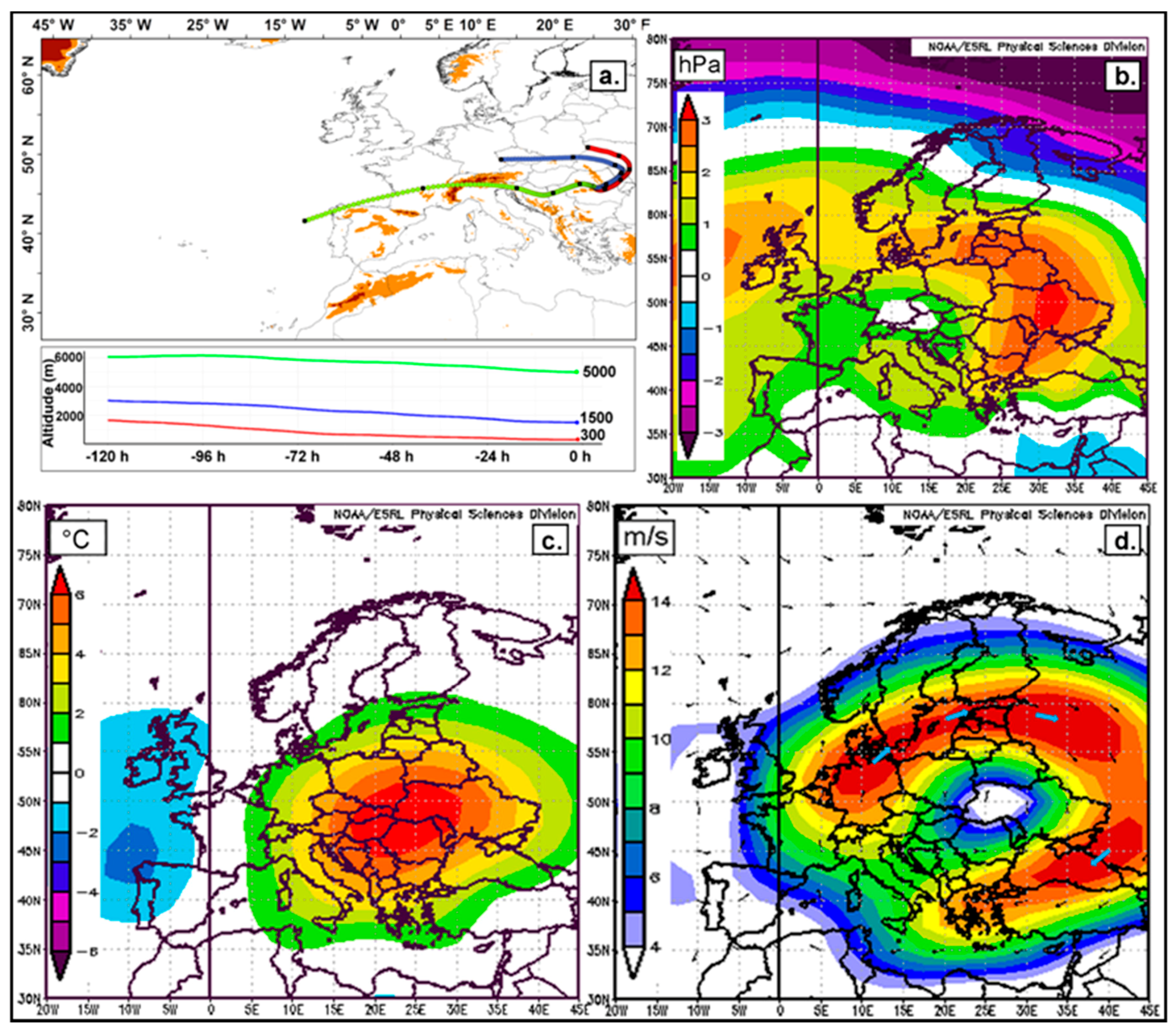
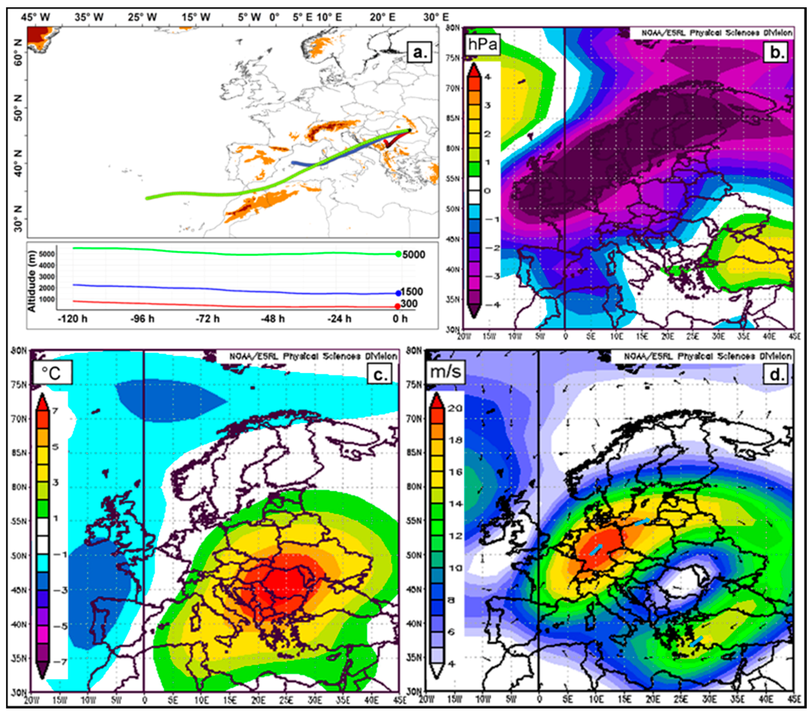
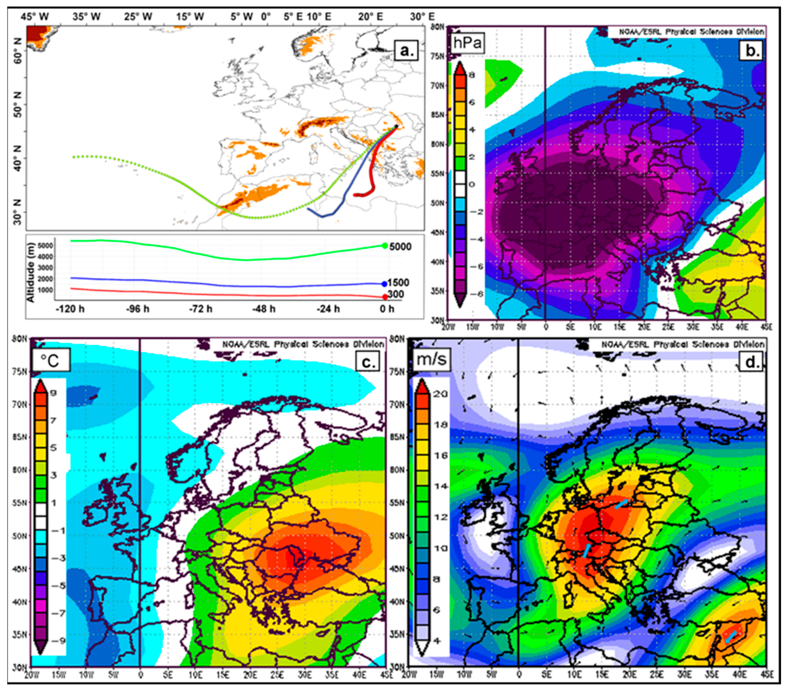
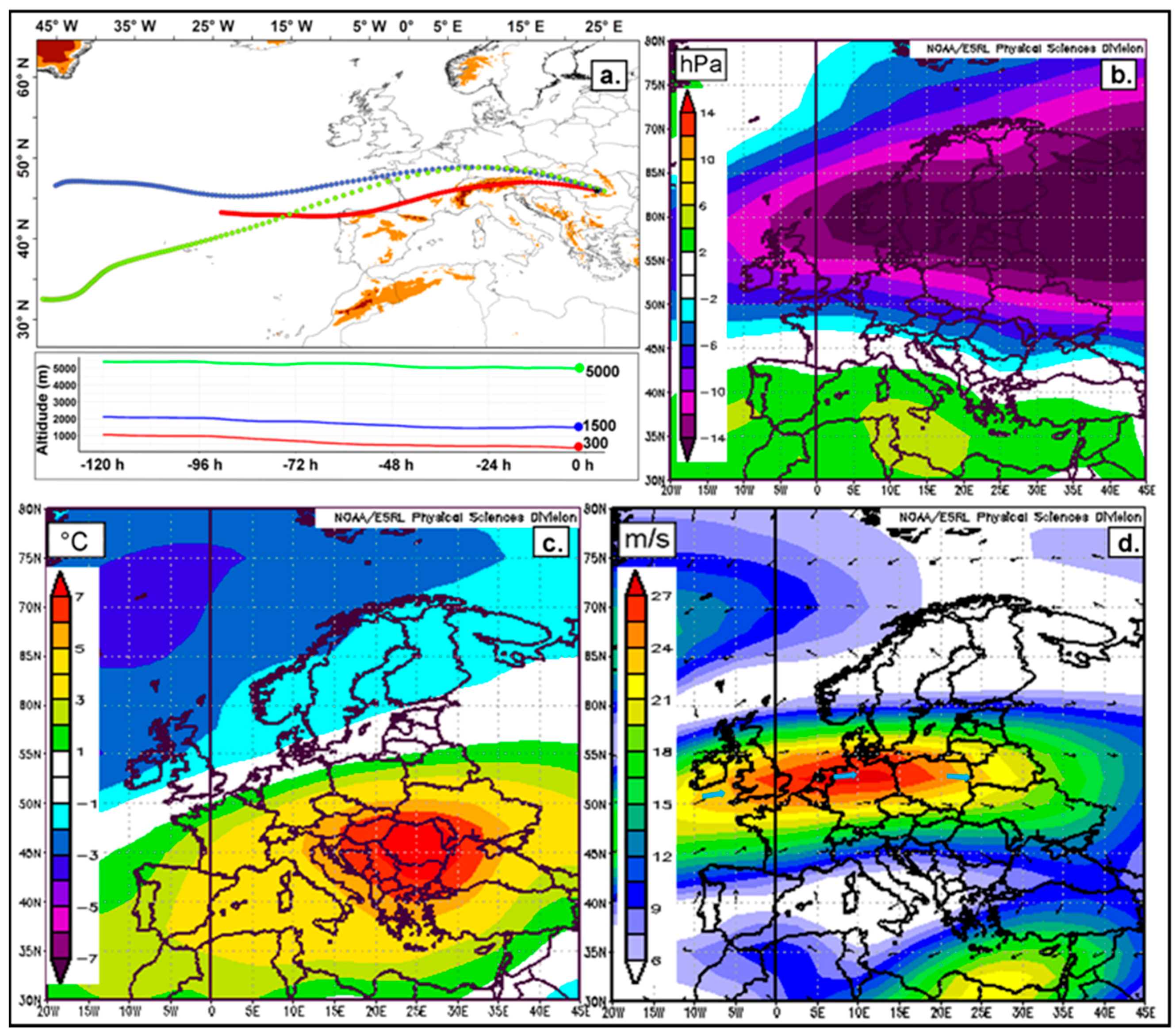
2.2.2. Synoptic Analysis

The synoptic classification of HW events was performed based on the analysis of daily issued synoptic maps at three geopotential levels: 300 hPa for jet stream trajectory, sea level pressure and 850 hPa for temperature advection, on the basis of the Earth System Research Laboratory composite maps tool from NOAA. In this section, the relationship between the HWs/WSs and the circulation conditions are analyzed using objective parameters of large-scale circulation patterns. Similar classifications were previously used by Unkašević and Tošić, [37,38].
In the first step, we considered the sea level pressure distribution in order to differentiate the main HW/WS types. Weak baric gradient over Romania is considered characteristic for A-type, considered as radiative–advective, while strong baric gradient was found specific for B-type, considered as advective–radiative. The threshold between weak and strong baric gradient is considered 4 hPa across Romania (approximately 0.5 hPa per 111 km).
In the second step, the origin of air masses generating HWs/WSs detected based on HYSPLIT trajectories was the criterion used to differentiate between sub-types of HWs, as used in other previous studies [36,72]. For A-type, anticyclonic curvature of trajectories was associated to A1-subtype (Figure 2a), while cyclonic curvature of trajectories was associated to A2-subtype (Figure 3a). The three sub-types of B-type HWs/WSs were identified based on the analysis of the spatial origins of the air masses: B1 was assumed to have North and Northeast African origins (Figure 4a), B2 was associated with Northwest Africa/Southwest Europe and subtropical North Atlantic origins (Figure 5a), while B3 was assumed to be with central North Atlantic origins (Figure 6a). Mean trajectories were computed based on all cases for each HW/WS sub-type (Figure 2a, Figure 3a, Figure 4a, Figure 5a and Figure 6a).
To identify the source regions of the air masses generating HWs/WSs, the atmospheric backward trajectories of the air particles have been simulated by employing the online version of HYSPLIT model Real-time Environmental Application and Display sYstem (READY), developed by researchers at the National Oceanic and Atmospheric Administration (NOAA) [57,58,73].
For this paper, we used backward trajectories detected at three levels, from near-ground level (0 m above ground level (AGL)) up to mid-troposphere (1500 and 5000 m AGL, respectively). By employing the vertical velocity option included in the HYSPLIT application, the vertical transport has been modeled for each 6-h intervals. The aforementioned levels were chosen to allow identification of possible different source-regions of air masses and the existence of different air masses in low and middle troposphere, respectively, over the considered region similarly to other studies. The trajectories of air particles were identified for the previous 120 hours of the first day of the HW/WS event. The backward trajectory was computed for the central area of Romania represented by the point located at 46°00′00″ N and 25°00′00″ E to identify the geographical area of air mass origins.
To fully describe each synoptic subtype, NCEP/NCAR reanalysis tool was used. The composite maps for SLP anomaly, 850 hPa temperature anomaly, and 300 hPa vector wind anomaly were obtained based on daily maps of the afore-mentioned variables for each HW subtype. Thus, we have a synthetic situation of synoptic conditions prior and during a HW event (analyzed based on five-day HYSPLIT backward trajectory and composite maps).
This analysis proved to be very useful for providing information needed to explain and classify conditions for HWs and WSs occurrence that could be of interest for the implementation of an early warning system.

3. Results and Discussion

3.1. Synoptic Classification of HWs/WSs in Romania

The synoptic conditions for HWs/WSs occurrence in Romania resulting from our analysis, can be divided into two major types:
(i) Radiative–advective HWs/WSs, for which radiative forcing plays the leading role in the occurrence of high temperature. For this type, solar heating, static stability, and the dryness of the air mass also play fundamental roles [14]. We shall refer to this HWs/WSs type as radiative HWs/WSs type to avoid any confusion.
(ii) Advective–radiative HWs/WSs for which the advection of a warm air mass plays the leading role for the occurrence of very high temperature. From now on, in this paper, we shall refer to this HWs/WSs type as advective HWs/WSs.
It is worth noting that no HWs/WSs occurred exclusively due to radiative or advective conditions. Both warm air mass advection and radiative forcing led to the occurrence of HWs/WSs. A second general synoptic characteristic of HWs/WSs is given by the fact that advection seems to be dominant in the process of HWs/WSs occurrence.

3.1.1. Synoptic Conditions Generating Radiative HWs/WSs

For the synoptic conditions generating radiative HWs/WSs two major subtypes were identified: Anticyclonic/Blocking High Conditions (A1) and Cyclonic/West European Upper Trough (A2). Generally, a weak advection of air masses is a common characteristic of typical HWs in the Balkans and Greece [26], as well as an increase in the stability of the atmospheric circulation that could partly explain the more frequent extreme air temperatures in Europe [43,44].
Subtype A1 is characterized by the following conditions:
(i) Anticyclonic curvature of backward trajectories indicating a general slow advection in the lower troposphere from northeasterly directions (Figure 2a) favored by the weak baric gradient, and a more intense southwesterly advection in the middle troposphere with its origins in Southwestern Europe.
(ii) High pressure conditions at sea level over Central and Southeastern Europe are associated very often with intense activity of Azores High during blocking circulation developed at a continental scale. Blocking conditions usually prevent cold fronts from bringing relief to the hot weather [14] and are well-known as an important factor for HWs/WSs occurrence in Europe [39]. This is the main dynamic cause for recording breaking HWs in Europe [74]. In addition, due to low advection, long-lasting high temperatures may support the development of high ridges in the mid-troposphere, which it is known as an important mechanism for this HW type action [1].
(iii) Warm high ridge associated to a positive air temperature anomaly at 850 hPa level (Figure 2b,c) becoming quasi-stationary in upper levels over Southeastern Europe with a negligible baric gradient at ground level over Romania.
(iv) The mean anomaly of wind vectors at 300 hPa during A1HW sub-type indicates high development of Rossby waves with a cut-off high structure centered over Romania; Central and Eastern Europe are located in the pole ward displacement of the jet stream that crosses with its axis over the Baltic Sea (Figure 2d); it is well-known that the persistence of HWs is determined by the presence of the long lasting upper tropospheric anticyclonic circulation [75]. Recently, Feudale [76] found that these conditions are probably enhanced by the positive anomaly of sea surface temperature of the Mediterranean Sea.
A similar synoptic pattern was identified as the main cause generating HWs over Central Europe [42] and the weak advection from Northeast under anticyclonic conditions is a common feature of the HWs in Southeast Europe [36].
From all 423 days cumulated by HWs/WSs in Romania identified during the period 1961–2015, 32.2% (136) of the days were characterized by this atmospheric circulation condition. The mean length of this HWs/WSs type is 3.7 days, while the maximum length was eight days (7–14 May 2003).
Subtype A2 is characterized by the following conditions:
(i) Cyclonic curvature of backward trajectories with a very slow advection generated by a weak gradient in the lower troposphere is associated with a stronger one in the upper level which has its origins in Southwestern Europe or Northwestern Africa (Figure 3a). This situation is also specific for Central-European HWs/WSs occurrence [42]. It generates important radiative warming, which represents, similar to A1 sub-type, an important contributor to the occurrence and persistence of high temperatures [1].
(ii) Weak negative pressure anomalies create conditions at sea level which prevail almost entirely over Europe, associated with a very weak baric gradient over the European continent; actually, this very weak gradient represents the main difference between this HWs/WSs sub-type and B2 HWs/WSs sub-type. In most cases, a center of low pressure can be identified over Great Britain, emphasized by the negative anomaly of 5 hPa on the map of sea level pressure, as well as at 850 hPa level (Figure 3b,c). A low pressure system, which is active over Great Britain and Northwest Europe was found to be the main center associated with HWs/WSs in Central Europe [42]. In addition, an important role seems to be played by a high pressure area, which is located over the Black Sea and Anatolia, leading to a weak southerly advection in the lower troposphere over Romania; this center is sustained by a weak convergence region on the upper level charts as depicted by the vector wind at 300 hPa (Figure 3d).
(iii) A strong ridge bringing very warm air masses in the upper level over Southeastern Europe in connection with a well-developed upper level trough over Western Europe is observed. These are separated by a strong jet stream, generally oriented from Southwestern toward Northeastern Europe.
From all 423 HWs/WSs days in Romania recorded over the period 1961–2015, 30.0% (127 days) were associated with this atmospheric circulation pattern. The mean length of HWs/WSs generated by this circulation type is 4.5 days, while the longest event reached 11 consecutive days (from 24 April to 4 May 2013).
Both sub-types of radiative HWs/WSs are associated with very warm ridges which are imposing a soil moisture deficit prior to the onset of the beginning of the HW/WS event [77], which is known as a main contributor to the increase in TX during HWs [78].

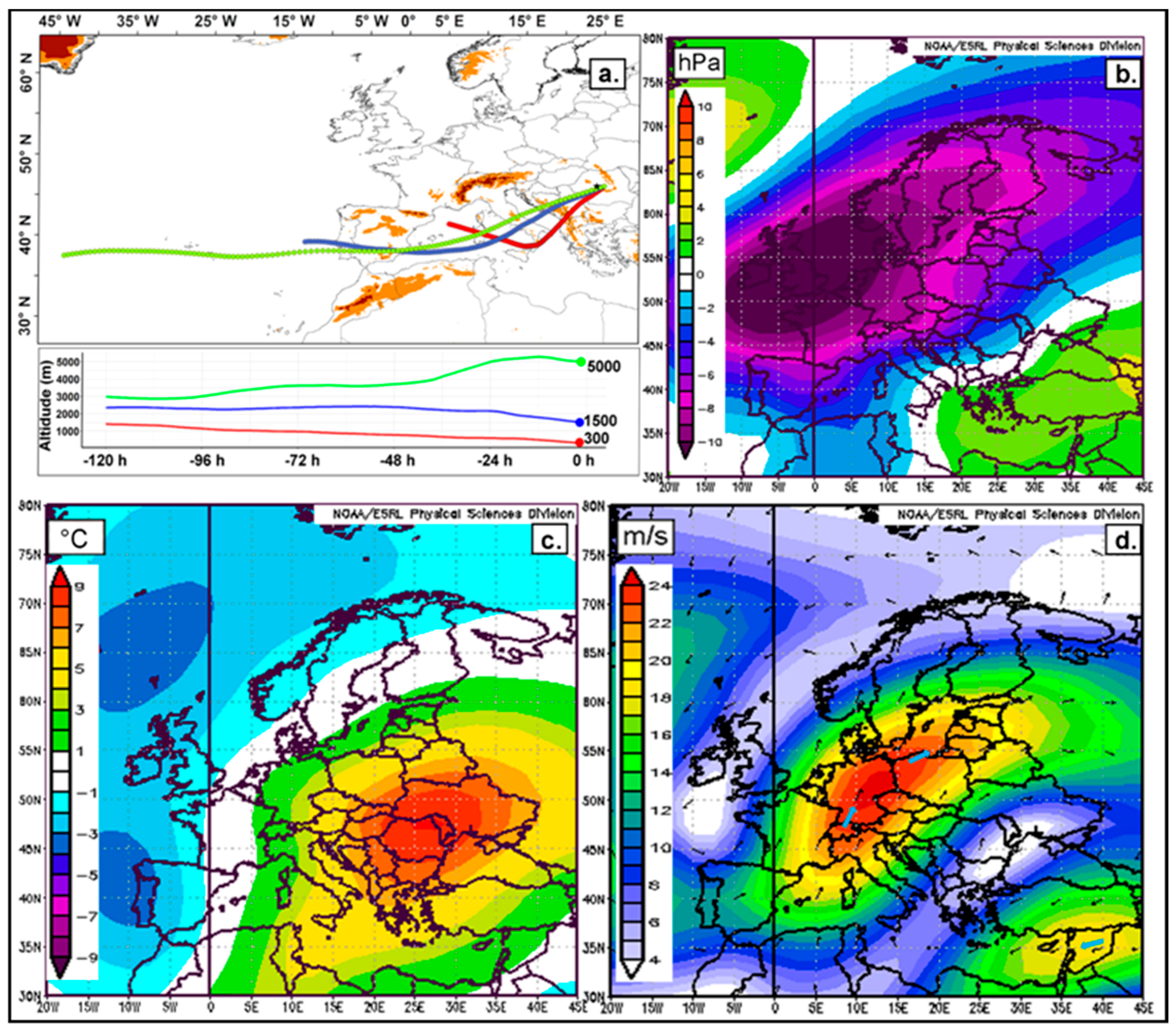
3.1.2. Synoptic Conditions Generating Advective HWs/WSs

The advective HWs/WSs can be also divided into three major sub-types according to the geographical origin of warm air mass advection: South (B1), Southwest (B2), and West (B3).
Subtype B1 is characterized by the following conditions:
(i) The backward trajectories indicate North African origins for the air particles in the previous five days, generally from the Libyan Desert at ground level, and from Northwestern Africa at 1500 m and 5000 m (Figure 4a–c);
(ii) A steep baric gradient covers the region of Romania, which is situated on the front Southeasterly side of low pressure systems centered over Central and Western Europe. At the same time, a high pressure field covers Southeastern Europe; these pressure patterns favor advection from South in the lower troposphere;
(iii) The jet stream splits over Europe into two branches that follow different trajectories: one goes over the subtropical regions and the other one over the Baltic Sea; in the region between these two branches, a positive temperature anomaly is characteristic over Southeast Europe including Romania (Figure 4d).
From the total number of HWs/WSs days detected in Romania for the 55-year period considered, 7.8% are associated with these atmospheric circulation conditions. This type of events has a mean duration of 3.8 days, while the maximum length was eight days (9–16 November 2010).
Subtype B2 is characterized by the following conditions:
(i) The backward trajectories indicate Southwest Europe and Northwest Africa origins for the air particle in the previous five days, generally from the Maghreb region at sea level and subtropical Atlantic origin for the lower and middle troposphere (Figure 5a–c).
(ii) A strong pressure gradient covers the region of Romania, which is located between some intense low pressure systems, acting over Northwestern Europe, and a high pressure field over Southeastern Europe. This synoptic pattern is also common for the HWs/WSs occurrence in Central Europe [42,79], and generates a strong Southwest advection in the lower troposphere. This is the main difference compared to A2 HWs/WSs type, which could be considered very similar.
(iii) The jet stream has the same spatial characteristics as for A2 HWs/WSs subtype (from Northwestern Africa toward Northeastern Europe) (Figure 5d), except for a higher speed, which determines a more intense advection in the lower troposphere.
This sub-type of synoptic conditions is responsible for 19.1% of the HWs/WSs days. The mean length of these HWs/WSs is 3.8 days, while their maximum length does not exceed five consecutive days.
North African high pressure advection processes were also found responsible for the most intense HWs occurrence in Serbia [37,38].
Sub-type B3 is characterized by the following conditions:
(i) The backward trajectories indicate Atlantic or even North American origin of the air particles associated with a very intense advection in connection with a zonal flow of the jet stream along the temperate zone (Figure 6a).
(ii) The subtropical warm ridge transition from Western toward Eastern Europe rather than a warm Atlantic air mass advection inside the continent (Figure 6b) leads to the positive temperature anomaly that covers the Mediterranean basin and Southern Romania (Figure 6c).
(iii) The Westerly flow conditions prevail over the entire continent, with high pressure systems covering Southern Europe and mobile Icelandic cyclones crossing North Europe from West to East (Figure 6d).
This sub-type of synoptic pattern is characteristic for 10.9% of days under HWs/WSs conditions. The mean length of these HWs/WSs is 3.5 days, with a maximum length not exceeding six consecutive days (1–6 December 1961).

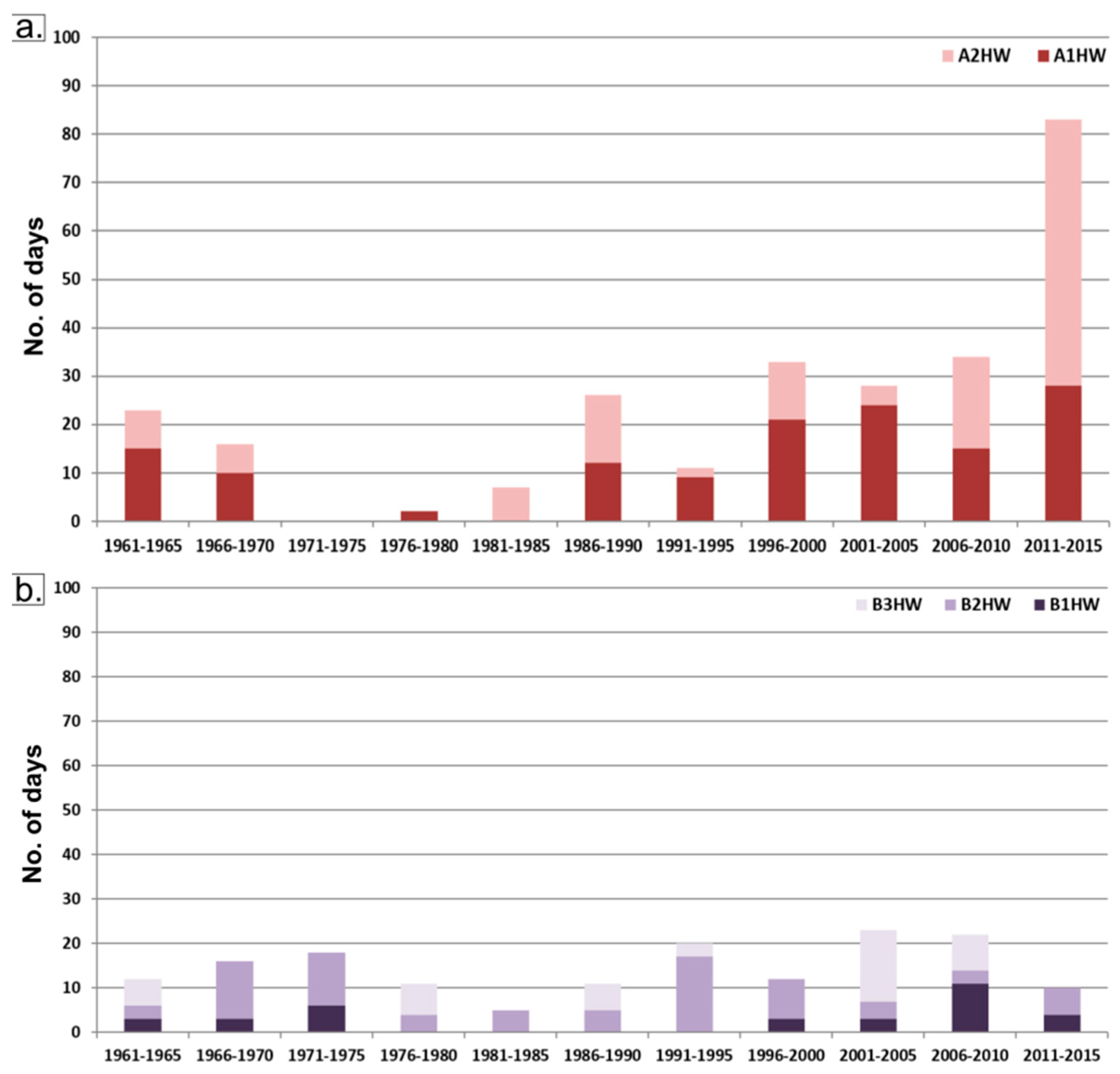
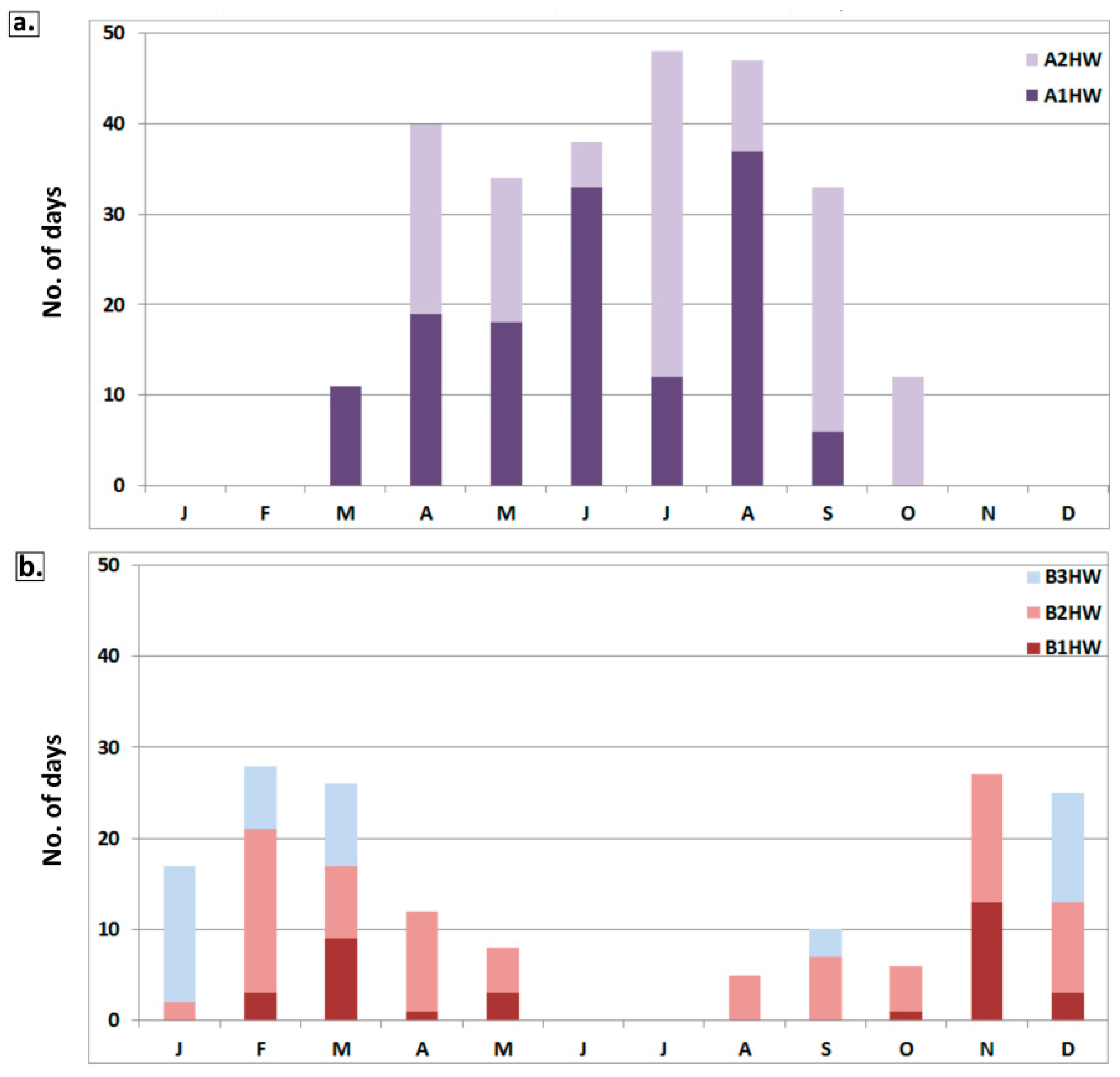
3.2. Frequency of HWs/WSs by Synoptic Conditions Types

According to scientific studies conducted in Europe or at global scale over the last two decades [6,37,38,42,69,80], the increasing frequency and intensity of HWs/WSs seem to be connected to the general trend observed in the temperature series along the second half of last century [81]. Tomczyk [36] revealed that in Southeast Europe, the increase of HWs/WSs frequency in the recent decades is at the highest level in Europe. This is confirmed also by our analysis, which indicates that 40% of the HWs/WSs days recorded in Romania, during the last 55 years are concentrated in the last 15 years (Figure 7). In this line, we can talk about an abrupt warming in the region rather than of a simple linear warming trend. The HWs/WSs represent a characteristic of the temperature variability all over the year [69,82], but their concentration is higher during the warm period. This fact is caused especially by the higher variability of the temperature during this period of the year. A third of the total number of days identified over the period 1961–2015, were concentrated in the summer, while the winter gathers only 16% of the days.
Generally, the first type of HWs/WSs (radiative) is more frequent during the warm season, while the second one is more common for the cold season (advective) (Figure 8). In spring and autumn, the HW/WS events develop both under advective (as also stated by Brunner et al. [39] for central Europe) and radiative conditions.

3.3. Intensity Features of HWs/WSs Associated to Each Synoptic Type

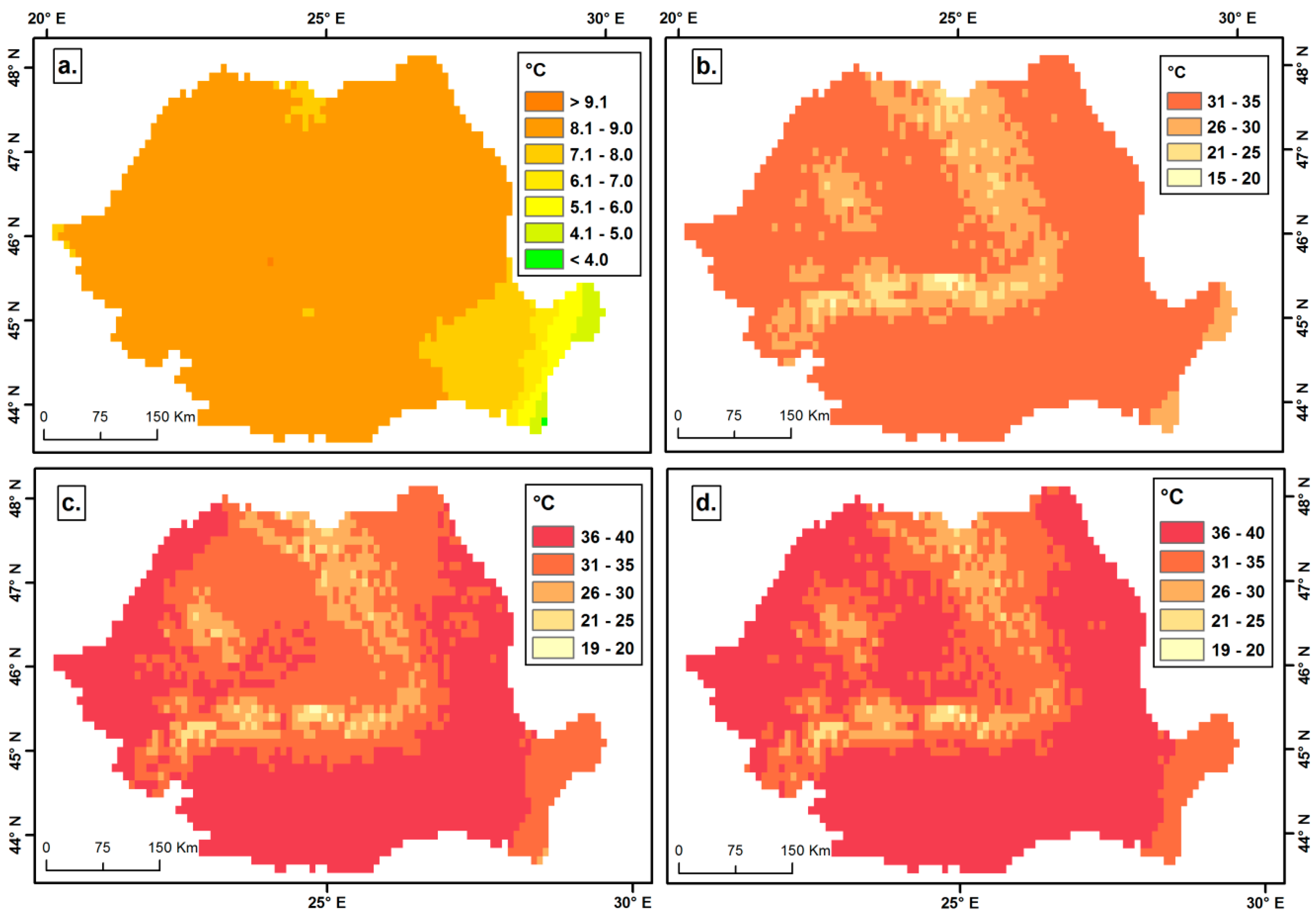
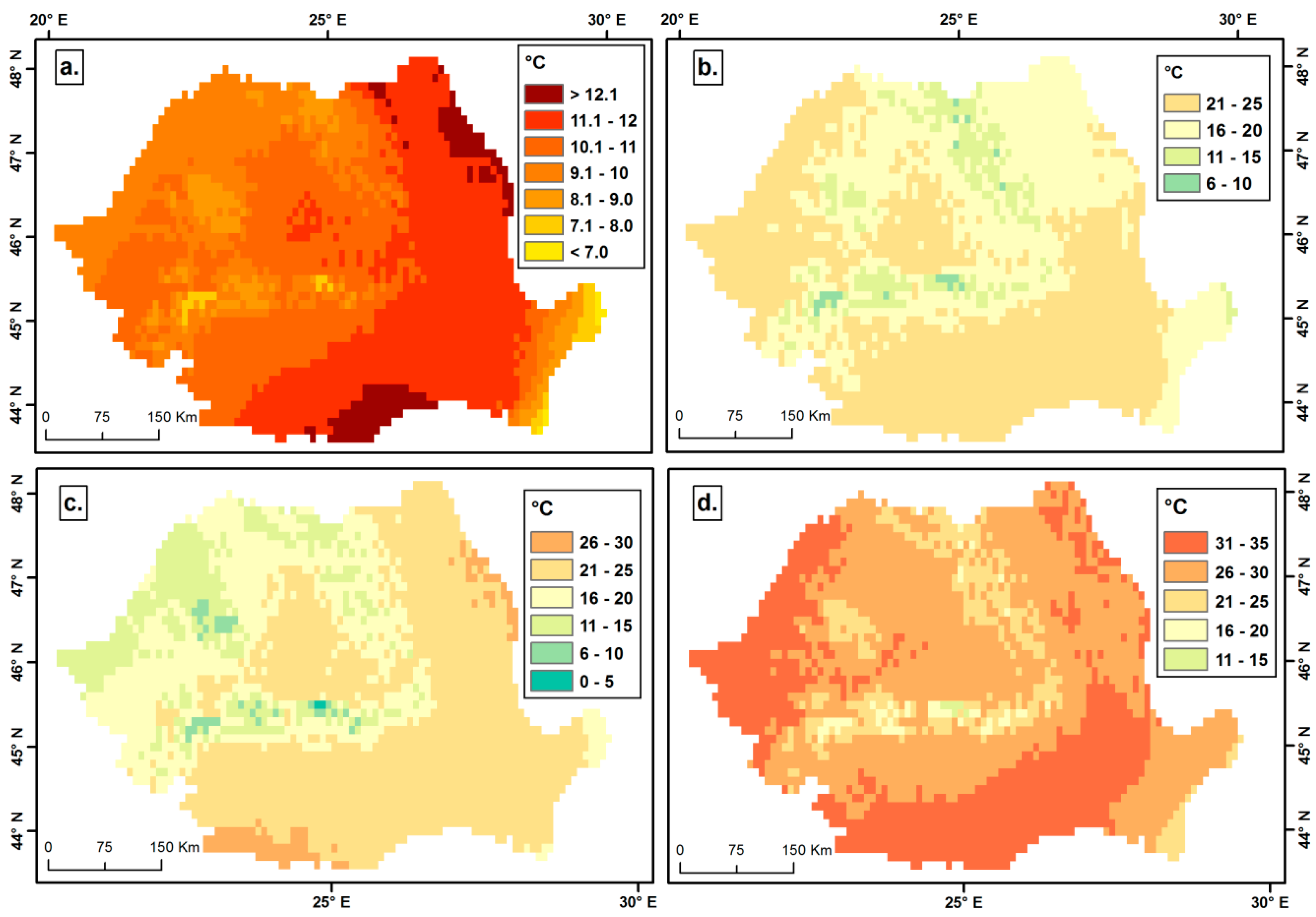
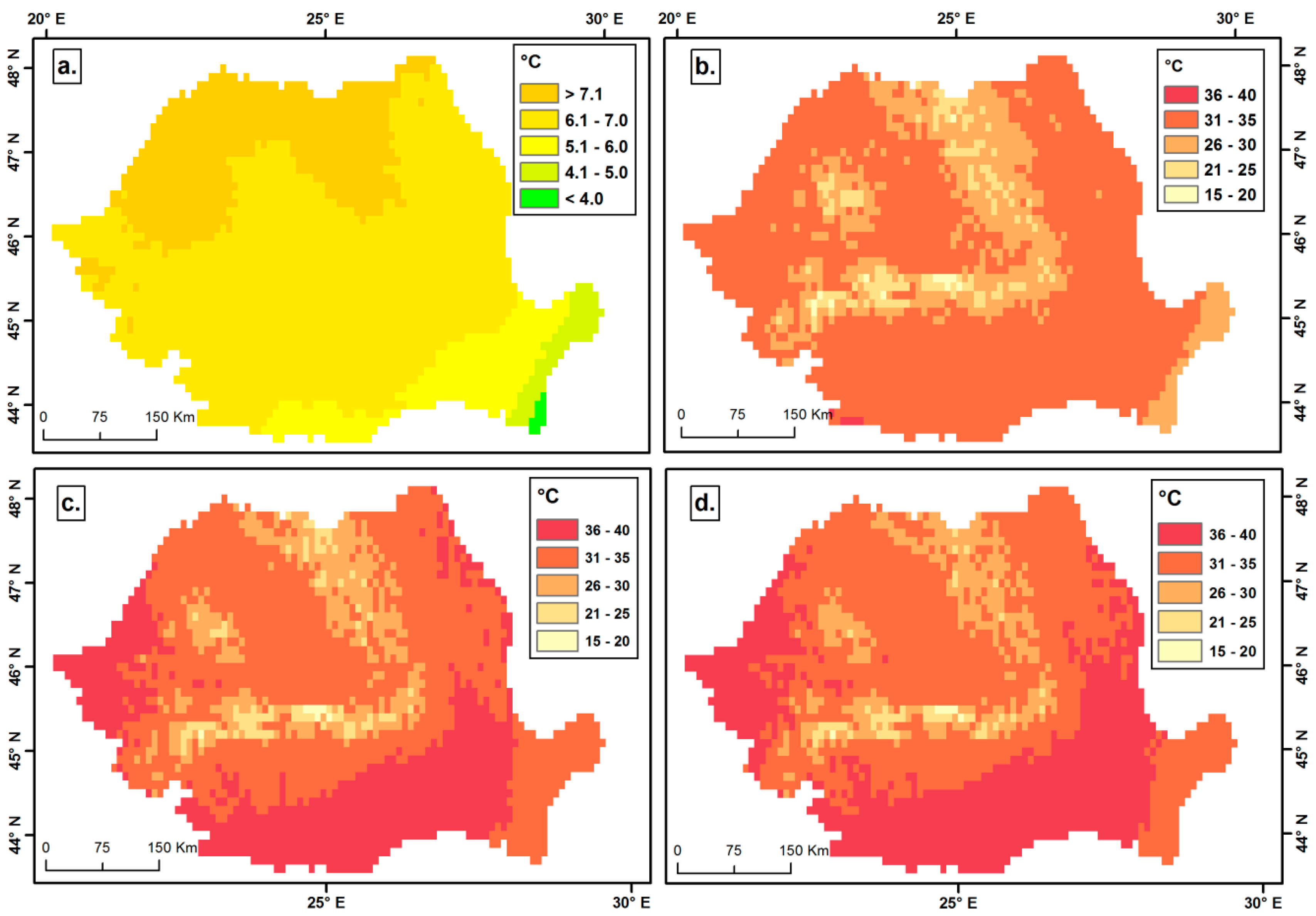
3.3.1. The Radiative HWs Characteristics

For A1 HWs/WSs type, the lowest positive anomaly occurs on the shoreline of the Black Sea, with less than 4 °C (Figure 9a) as a result of the large water body influence, especially in June (Figure 9b). The lowest TX is specific to the mountain area, with daily average values below 20 °C, recorded on the highest peaks of the Carpathians and 20–25 °C in the mid-height mountains. This fact sustains the contribution of the radiative processes for high temperature occurrences because of the intense loss of solar radiation in the mountain area seems to be responsible for weaker anomalies recorded in those areas. A1 HWs/WSs type was characterized by temperatures which generally exceed 35 °C during summer in the lowlands of Romania, especially in July and August (Figure 9c,d), a value which corresponds to a pronounced positive anomaly for TX. The maximum anomaly, of more than 7 °C was found in North and Northwest Romania, and underlines the North to South homogenization of TX in Romania during summer HWs. This pattern of positive anomaly across Romania is explained by the mean position of a warm ridge and an anticyclonic center over central Europe during A1 HWs/WSs type (Figure 3).
The circulation pattern of A2 HWs/WSs type generates a more uniform spatial distribution of TX anomalies over the entire country (Figure 10), which usually do not exceed 10 °C. This situation is caused mainly by the intense warm ridge, which prevails in the lower and middle troposphere causing an intense warm advection both at low and high altitudes.
These synoptic conditions lead to temperatures that exceed 40 °C, values which are close to the absolute maximum temperature recorded in the country (44.5 °C). It is very important to highlight the abrupt increasing frequency of this heat events in the last decade, which must be considered as a signal for the higher frequency of the occurrence of long lasting hot days during summer, in the region. The mean maximum daily temperatures for this HWs sub-type are higher than for A1 HW sub-type due to the higher temperature at altitude. At ground level, values greater than 35 °C were encountered in July and August in the Transylvanian Basin.
Another characteristic related to this HWs sub-type is represented by the lower maximum air positive anomaly over southeastern Romania. The maximum temperature is moderated by the large water body of the Black Sea, such as for A1 HWs. This time a more pronounced temperature along the shoreline in July and August (Figure 10c,d) is specific. The lower temperature is associated with the sea breeze mechanism which can develop more intensively during A2 HWs than during A1 HWs due to the lower baric gradient. Under these conditions, the daily maximum temperature along the Black Sea coast is just a few degrees above 30 °C, while in the central part of the Danube Plain or along the Danube valley the mean maximum temperature can rise up to 35 °C, or even 40 °C.

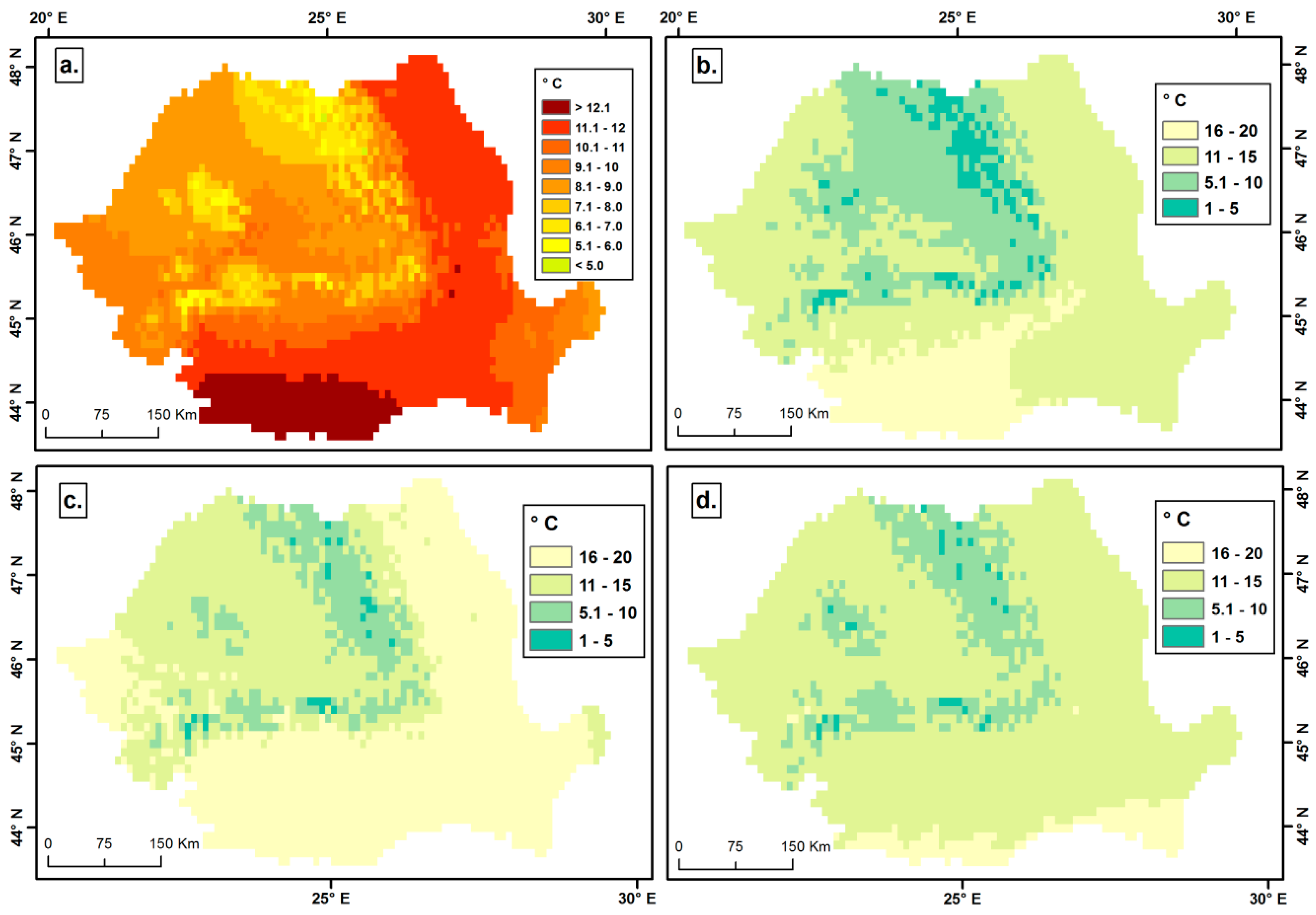
3.3.2. The Advective HWs/WSs Characteristics

B1 and B2 HWs/WSs types have a quite similar impact in terms of spatial distribution of daily maximum temperatures in Romania, even though the synoptic conditions are different (as presented before). For these two types of HWs/WSs, the positive anomaly of maximum temperatures usually exceeds 11 °C (Figure 11a and Figure 12a) in eastern Romania, while mean maximum temperature are much higher compared to the mean values of the period (Figure 11b–d and Figure 12b–d).
Under these circumstances, the temperatures seem to be comfortable for the human body, but they become very dangerous when they occur in transitional seasons, especially when they cause an early germination of the plants in March–April, making them extremely vulnerable to the late frost that can occur until late April or even May.
The axes of the warm ridges, which characterize these HWs types, pass over the southern and eastern parts of Romania; the anomaly in the northwestern part of the country is lower because of their peripheral position in relation to the axis. We should emphasize that the southern and eastern parts of the country are more susceptible to the warm air masses’ advection than the northwestern part of the country.
In the case of B1 HWs sub-type with closer origins to the tropical air masses (Libyan or Algerian Sahara), the positive anomaly exceeds 13 °C in the lowlands in the South and Northeast of Romania. Under these circumstances, maximum temperatures up to 30 °C can occur in April or October (Figure 11c), while, in May or September, values higher than 30 °C are quite frequent. For B2 HW sub-type, with a more pronounced Southwest airflow, the mean maximum temperature is higher in the South and West of Romania (31–35 °C), while in the Northeast the mean maximum temperature does not exceeds 30 °C (Figure 12d).
It is important to note that the maximum positive anomaly occurs isolatedly in the regions located at the eastern and southern periphery of the Carpathians (Sub-Carpathian region), a pre-mountain region, where the warm advection is more important than in the Danube Plain where haze, fog or even low clouds can diminish the temperature increase in spring or autumn.
The low positive anomalies near the Black Sea coastline for both HWs/WSs sub-types are a consequence of low clouds and fog, which develop as a result of mixture between the warm air advection and the cooler air mass specific in low layers over the waters of the Black Sea. The frequency of fog and low clouds is the highest along the shoreline of the Black Sea from February to April [83], when these two WSs types have the highest frequency, too. The lowest positive anomaly recorded in the Danube Delta (2–3 °C above normal) is a direct indicator of this mechanism.
During winter the most intense WSs are caused by an intense Westerly circulation, indicated here as B3 WSs type (Figure 13). This sub-type of atmospheric circulation is known to bring positive deviation in the field of air temperature over Romania, especially in winter [84] and sometimes, the increase in air temperature is high enough to include the events in the WSs category.
Under these conditions, the highest positive anomaly was recorded in southwestern Romania and locally near the curvature of the Romanian Carpathians (Figure 13a). The last region may be an indicator of the role played by the foehn effect of the Westerly flow crossing over the mountains, reflected in the mean maximum temperature in December (Figure 13b). High anomalies are also specific in the northeast of the country, a region prone to the westerly circulation.
The lower maximum temperature, in the winter, in southeastern Romania is generated by the proximity of the Black Sea, especially in the region of the Danube Delta.
The positive anomalies are lower in Northern Carpathians and generally in central and Northwestern Romania because of the Westerly circulation which brings colder polar air masses from the North Atlantic, while eastern and southern Romania are still under the influence of the warm air advected previously from Central and Western Europe. In addition, intense thermal inversions can develop in the mountain depressions in northwestern Romania under warm air advection conditions induced by the Westerly circulation, and resulting in lower maximum temperatures than outside the Carpathian Mountains.

4. Conclusions

Europe has had many recent instances of unprecedented HWs affecting large populated areas with very high mortality rates, particularly in the summers of 2003 and 2006 [14,24,85,86,87]. In this paper, we bring a large scale perspective to the HWs/WSs occurrence conditions in Romania, but these results can also be useful for some neighboring regions.
In this paper, we identified two main types and five sub-types of synoptic conditions generating HWs/WSs. We found that, in summer, HWs are induced by positive or neutral sea level pressure anomalies, with major role played by strong and persistent well-developed ridges and their ability to push moisture pole ward along their western branch. During other seasons, the cyclonic conditions associated with intense advections are common. A steep increase of the HWs/WSs days during the last 15 years must be highlighted as a possible indicator of the future evolution of these types of extreme weather events.
These results can become a useful tool for weather forecasters to better predict the occurrence of HWs/WSs as well as to different stakeholders acting in health and public transportation systems or energy supplying systems due to the multitude of negative impact types induced by HWs/WSs.

Acknowledgments

This research was developed under the framework of the research grant Extreme weather events related to air temperature and precipitation in Romania (project code: PN-II-RU-TE-2014-4-0736), funded by the Executive Unit for Financing Higher Education, Research, Development, and Innovation (UEFISCDI) in Romania. The funds of the project do not cover the open access publication. The authors acknowledge the daily temperature data provided by the European Climate Assessment & Dataset project [55], Meteomanz data base, and the National Meteorological Administration in Romania data base for direct measurements and gridded data [56]. The authors gratefully acknowledge the NOAA Air Resources Laboratory (ARL) for the provision of the HYSPLIT transport and dispersion model and/or READY website (http://www.ready.noaa.gov) used in this publication. The authors kindly acknowledge the three anonymous reviewers for their useful comments and suggestions.

Author Contributions

Lucian Sfica and Adina-Eliza Croitoru conceived and designed the paper; Adina-Eliza Croitoru and Flavius-Antoniu Ciupertea performed the data processing for identification of HWs/WSs; Lucian Sfica and Iulian Iordache analyzed the synoptic data; and Lucian Sfica and Adina-Eliza Croitoru wrote the paper.

Conflicts of Interest

The authors declare no conflict of interest.

References

  1. Huth, R.; Kysely, J.; Pokorna, L. A GCM simulation of heat waves, dry spells, and their relationships to circulation. Climatic Change 2000, 46, 29–60. [Google Scholar] [CrossRef]
  2. Beniston, M. The 2003 heat wave in Europe: A shape of things to come? An analysis based on Swiss climatological data and model simulations. Geophys. Res. Lett. 2004, 31, 202. [Google Scholar] [CrossRef]
  3. Meehl, G.; Tebaldi, C. More intense, more frequent, and longer lasting heat waves in the 21st century. Science 2004, 305, 994–997. [Google Scholar] [CrossRef] [PubMed]
  4. Schär, C.; Vidale, P.; Luthi, D.; Frei, C.; Haberli, C.; Liniger, M.; Appenzeller, C. The role of increasing temperature variability in European summer heatwaves. Nature 2004, 427, 332–336. [Google Scholar] [CrossRef] [PubMed]
  5. Stott, P.; Stone, D.; Allen, M. Human contribution to the European heatwave of 2003. Nature 2004, 432, 610–614. [Google Scholar] [CrossRef] [PubMed]
  6. Della-Marta, P.M.; Luterbacher, J.; von Weissenfluh, H.; Xoplaki, E.; Brunet, M.; Wanner, H. Summer heat waves over western Europe 1880–2003, their relationship to large-scale forcings and predictability. Clim. Dyn. 2007, 29, 251–275. [Google Scholar] [CrossRef]
  7. Coumou, D.; Rahmstorf, S. A decade of weather extremes. Nat. Clim. Change 2012, 2, 491–496. [Google Scholar] [CrossRef]
  8. Perkins, S.E.; Alexander, L.V. On the measurement of heat waves. J. Clim. 2013, 26, 4500–4517. [Google Scholar] [CrossRef]
  9. Peterson, T.C.; Heim, R.R., Jr.; Hirsch, R.; Kaiser, D.P.; Brooks, H.; Diffenbaugh, N.S.; Dole, R.M.; Giovannettone, J.P.; Guirguis, K.; Karl, T.R.; et al. Monitoring and understanding changes in heat waves, cold waves, floods, and droughts in the United States: State of knowledge. Bull. Amer. Meteor. Soc. 2013, 94, 821–834. [Google Scholar] [CrossRef]
  10. Keellings, D.; Waylen, P. Increased risk of heat waves in Florida: Characterizing changes in bivariate heat wave risk using extreme value analysis. Appl. Geogr. 2014, 46, 90–97. [Google Scholar] [CrossRef]
  11. Keggenhoff, I.; Elizbarashvili, M.; King, L. Heat wave events over Georgia since 1961: Climatology, changes and severity. Climate 2015, 3, 308–328. [Google Scholar] [CrossRef]
  12. Rusticucci, M.; Kyselý, J.; Almeira, G.; Lhotka, O. Long-term variability of heat waves in Argentina and recurrence probability of the severe 2008 heat wave in Buenos Aires. Theor. Appl. Climatol. 2016, 124, 679–689. [Google Scholar] [CrossRef]
  13. Croitoru, A.-E.; Piticar, A.; Ciupertea, A.F.; Roşca, C.F. Changes in heat waves indices in Romania over the period 1961–2015. Glob. Planet. Change 2016, 146, 109–121. [Google Scholar] [CrossRef]
  14. Pezza, A.-B.; van Rensch, P.; Cai, W. Severe heat waves in the Southern Australia: Synoptic climatology and large scale connections. Clim. Dyn. 2012, 38, 209–224. [Google Scholar] [CrossRef]
  15. Meehl, G.A.; Karl, T.; Easterling, D.R.; Changnon, S.; Pielke, R.J.; Changnon, D.; Evans, J.; Groisman, P.Y.; Knutson, T.R.; Kunkel, K.E.; et al. An introduction to trends in extreme weather and climate events: Observations, socioeconomic impacts, terrestrial ecological impacts, and model projections. Bull. Am. Meteorol. Soc. 2000, 81, 413–416. [Google Scholar] [CrossRef]
  16. Heatwaves: Risks and responses. Available online: http://www.euro.who.int/en/publications/abstracts/heat-waves-risks-and-responses (accessed on 27 September 2016).
  17. Managing the risks of extreme events and disasters to advance climate change adaptation. Available online: https://www.ipcc.ch/pdf/special-reports/srex/SREX_Full_Report.pdf (accessed on 27 September 2016).
  18. Radinović, D.; Ćurić, M. Criteria for heat and cold wave duration indexes. Theor.Appl. Climatol. 2012, 107, 505–510. [Google Scholar] [CrossRef]
  19. Giles, B.D.; Balafoutis, C.J. The Greek Heat Waves of 1987 and 1988. Int. J. Climatol. 1990, 10, 505–517. [Google Scholar] [CrossRef]
  20. Giles, B.D.; Balafoutis, C.; Maheras, P. Too hot for comfort: The heat waves in Greece in1987 and 1988. Int. J. Biometeorol. 1990, 34, 98–104. [Google Scholar] [CrossRef] [PubMed]
  21. Matzarakis, A.; Mayer, H. Heat stress in Greece. Int. J. Biometeorol. 1997, 41, 34–39. [Google Scholar] [CrossRef] [PubMed]
  22. Pantavou, K.; Theoharatos, G.; Nikolopoulos, G.; Katavoutas, G.; Asimakopoulos, D. Evaluation of thermal discomfort in Athens territory and its effect on the daily number of recorded patients at hospitals’ emergency rooms. Int. J. Biometeorol. 2008, 52, 773–778. [Google Scholar] [CrossRef] [PubMed]
  23. Dolney, T.J.; Sheridan, S.C. The relationship between extreme heat and ambulance response calls for the city of Toronto, Ontario, Canada. Environ. Res. 2006, 101, 94–103. [Google Scholar] [CrossRef] [PubMed]
  24. Fouillet, A.; Rey, G.; Laurent, F.; Pavillon, G.; Bellec, S.; Guihenneuc-Jouyaux, C.; Clavel, J.; Jougla, E.; Hémon, D. Excess mortality related to the August 2003 heatwave in France. Int. Arch. Occup. Environ. Health 2006, 80, 16–24. [Google Scholar] [CrossRef] [PubMed] [Green Version]
  25. Basu, R.; Samet, J.M. Relation between elevated ambient temperature and mortality: Are view of the epidemiologic evidence. Epidemiol. Rev. 2002, 24, 190–202. [Google Scholar] [CrossRef] [PubMed]
  26. Theoharatos, G.; Pantavou, K.; Mavrakis, A.; Spanou, G.-K.; Efsthatiou, P.; Mpekas, P.; Asimakopoulos, D. Heat waves observed in 2007 in Athens, Greece: Synoptic conditions, bioclimatological assessement, air quality levels and health effects. Environ. Res. 2010, 110, 152–161. [Google Scholar] [CrossRef] [PubMed]
  27. De Bono, A.; Giuliani, G.; Kluser, S.; Peduzzi, P. Impacts of summer 2003 heat wave in Europe. Eur. Environ. Alert. Bull. 2004, 2, 1–4. [Google Scholar]
  28. Russo, S.; Sillmann, J.; Fischer, E.M. Top ten European heatwaves since 1950 and their occurrence in the coming decades. Environ. Res. Lett. 2015, 10, 124003. [Google Scholar] [CrossRef]
  29. Colman, A. Prediction of summer central England temperature from preceding North Atlantic winter sea surface temperature. Int. J. Climatol. 1997, 17, 1285–1300. [Google Scholar] [CrossRef]
  30. Enfield, D.B.; Mestas-Nunez, A.M.; Trimble, P.J. The Atlantic multidecadal oscillation and its relation to rainfall and river flows in the continental US. Geophys. Res. Lett. 2001, 28, 2077–2080. [Google Scholar] [CrossRef]
  31. Kysely, J. Temporal fluctuations in heat waves at Prague-Klementinum, the Czech Republic, from 1901–1997, and their relationships to atmospheric circulation. Int. J. Climatol. 2002, 22, 33–50. [Google Scholar] [CrossRef]
  32. Cassou, C.; Terray, L.; Phillips, A.S. Tropical Atlantic Influence on European Heat Waves. J. Clim. 2005, 18, 2805–2811. [Google Scholar] [CrossRef]
  33. Sutton, R.T.; Hodson, D.L.R. Atlantic Ocean forcing of North American and European summer climate. Science 2005, 309, 115–118. [Google Scholar] [CrossRef] [PubMed]
  34. Nakamura, M.; Enomoto, T.; Yamane, S. A simulation study of the 2003 heatwave in Europe. J. Earth. Simul. 2005, 2, 55–69. [Google Scholar]
  35. Teng, H.; Branstator, G.; Wang, H.; Meehl, G.A.; Washington, W.M. Probability of US heat waves affected by a subseasonal planetary wave pattern. Nat. Geosci. 2013, 6, 1056–1061. [Google Scholar] [CrossRef]
  36. Tomczyk, A.M. Impact of atmospheric circulation on the occurrence of heat waves in southeastern Europe. Időjárás 2016, 120, 395–414. (In Magyar) [Google Scholar]
  37. Unkašević, M.; Tošić, I. An analysis of heat waves in Serbia. Glob. Planet. Change 2009, 65, 17–26. [Google Scholar] [CrossRef]
  38. Unkašević, M.; Tošić, I. Seasonal analysis of cold and heat waves in Serbia during the period 1949–2012. Theor. Appl. Climatol. 2015, 120, 29–40. [Google Scholar] [CrossRef]
  39. Brunner, L.; Hegerl, G.; Steiner, A. Connecting Atmospheric Blocking to European Temperature Extremes in Spring. J. Clim. 2017, 30, 585–594. [Google Scholar] [CrossRef]
  40. Leckebusch, G.C.; Ulbrich, U. On the relationship between cyclones and extreme windstorms over Europe under climate change. Glob. Planet. Change 2004, 44, 181–193. [Google Scholar] [CrossRef]
  41. Leckebusch, G.C.; Weimer, A.; Pinto, J.G.; Reyers, M.; Speth, P. Extreme wind storms over Europe in present and future climate: A cluster analysis approach. Meteorol. Z. 2008, 17, 67–82. [Google Scholar]
  42. Tomczyk, A.M.; Bednorz, E. Heat waves in Central Europe and their circulation conditions. Int. J. Climatol. 2016, 36, 770–782. [Google Scholar] [CrossRef]
  43. Kysely, J.; Domonkos, P. Recent increase in persistence of atmospheric circulation over Europe: Comparison with long-term variations since 1881. Int. J. Climatol. 2006, 26, 461–483. [Google Scholar] [CrossRef]
  44. Kysely, J. Implications of enhanced persistence of atmospheric circulation for the occurrence and severity of temperature extremes. Int. J. Climatol. 2007, 27, 689–695. [Google Scholar] [CrossRef]
  45. Kysely, J. Influence of the persistence of circulation patterns onwarm and cold temperature anomalies in Europe: Analysis over the 20th century. Glob. Planet. Change 2008, 62, 147–163. [Google Scholar] [CrossRef]
  46. Porebska, M.; Zdunek, M. Analysis of extreme temperature events in Central Europe related to high pressure blocking situations in 2001–2011. Meteorol. Z 2013, 22, 533–540. [Google Scholar]
  47. Donat, M.G.; Alexander, L.V.; Yang, H.; Durre, I.; Vose, R.; Robert, J.H.D.; Katharine, M.W.; Enric, A.; Manola, B.; Caesar, J.; et al. Updated analyses of temperature and precipitation extreme indices since the beginning of the twentieth century: The HadEX2 dataset. J. Geophys. Res. Atmos. 2013, 118, 2098–2118. [Google Scholar] [CrossRef]
  48. Spinoni, J.; Lakatos, M.; Szentimrey, T.; Bihari, Z.; Szalai, S.; Vogt, J.; Antofie, T. Heat and cold waves trends in Carpathian Region from 1961 to 2010. Int. J. Climatol. 2015, 35, 4197–4209. [Google Scholar] [CrossRef]
  49. Dragotă, C.-S.; Havriş, L.-E. Changes in Frequency, persistence and intensity of extreme high-temperature events in the Romanian Plain. In Proceedings of Air and water—Components of the Environment, Cluj, Romania, 20–22 March 2015.
  50. Huștiu, M.C. Cold and heat waves in the Barlad Plateau between 1961 and 2013. Riscuri şi Catastrofe 2016, 18, 31–42. [Google Scholar]
  51. Croitoru, A.-E.; Antonie, R.I.; Rus, A. Heat waves and their estimated socio-economic impact in Bucharest city, Romania. In Proceedings of the 14th International Multidisciplinary Scientific GeoConference SGEM2014, Sofia, Bulgaria, 7–26 June 2014; pp. 367–374.
  52. Papathoma-Koehle, M.; Promper, C.; Bojariu, R.; Cica, R.; Sik, A.; Perge, K.; Laszlo, P.; Balazs, C.E.; Dumitrescu, A.; Turcus, C.; et al. A common methodology for risk assessment and mapping for south-east Europe: An application for heat wave risk in Romania. Nat. Hazards 2016. [Google Scholar] [CrossRef]
  53. Croitoru, A.-E.; Piticar, A.; Burada, D.C. Changes in precipitation extremes in Romania. Quatern. Int. 2016, 415, 325–335. [Google Scholar] [CrossRef]
  54. Guide to Climatological Practices. Available online: http://www.wmo.int/pages/prog/wcp/ccl/guide/documents/WMO_100_en.pdf (accessed on 22 January 2017).
  55. Klein Tank, A.M.G.; Wijngaard, J.B.; Konnen, G.P.; Böhm, R.; Demaree, G.; Gocheva, A.; Mileta, M.; Pashiardis, S.; Hejkrilik, L.; Kern-Hansen, C.; et al. Daily dataset of 20th-century surface air temperature and precipitation series for the European climate assessment. Int. J. Climatol. 2002, 22, 1441–1453. [Google Scholar] [CrossRef]
  56. Dumitrescu, A.; Birsan, M.V. ROCADA: A gridded daily climatic dataset over Romania (1961–2013) for nine meteorological variables. Nat. Hazards 2015, 78, 1045–1063. [Google Scholar] [CrossRef]
  57. Stein, A.F.; Draxler, R.R.; Rolph, G.D.; Stunder, B.J.B.; Cohen, M.D.; Ngan, F. NOAA’s HYSPLIT atmospheric transport and dispersion modeling system. Bull. Amer. Meteor. Soc. 2015, 96, 2059–2077. [Google Scholar] [CrossRef]
  58. Real-time Environmental Applications and Display sYstem (READY). Available online: https://www.ready.noaa.gov/index.php (accessed on 16 October 2016).
  59. Ustrnul, Z.; Czekierda, D. Atlas of Extreme Meteorological Phenomena and Synoptic Situations in Poland; Instytut Meteorologii i Gospodarki Wodnej: Warszawa, Poland, 2009; pp. 1–182. [Google Scholar]
  60. Furrer, E.M.; Katz, R.W.; Walter, M.D.; Furrer, R. Statistical modeling of hot spells and heat waves. Clim. Res. 2010, 43, 191–205. [Google Scholar] [CrossRef]
  61. Croitoru, A.-E. Heat waves. Concept, definition and methods used to detect. Riscuri și Catastrofe 2014, XV(2), 25–32. [Google Scholar]
  62. Kyselý, J. Probability estimates of extreme temperature events: Stochastic.modelling approach vs. extreme value distributions. Stud. Geophys. Geod. 2002, 46, 93–112. [Google Scholar] [CrossRef]
  63. Kossowska-Cezak, U. Fale upałów i okresy upalne-metody ich wyróżniania i wyniki zastosowania. Prace Geograficzne 2010, 123, 143–149. (In Polski) [Google Scholar]
  64. Bobvos, J.; Fazekas, B.; Páldy, A. Assessment of heat-related mortality in Budapest from 2000 to 2010 by different indicators. Időjárás 2015, 119, 143–158. (In Magyar) [Google Scholar]
  65. Kuchcik, M.; Degórski, M. Heat- and cold-related mortality in the north-east of Poland as an example of the socio-economic effects of extreme hydrometeorological events in the Polish Lowland. Geographia Polonica. 2009, 82, 69–78. [Google Scholar] [CrossRef]
  66. Frich, P.; Alexander, L.V.; Della-Marta, P.; Gleason, B.; Haylock, M.; Klein Tank, A.M.G.; Peterson, T. Observed coherent changes in climatic extremes during 2nd half of the 20th century. Clim. Res. 2002, 19, 193–212. [Google Scholar] [CrossRef]
  67. Palecki, M.A.; Changnon, S.A.; Kunkel, K.E. The Nature and Impacts of the July 1999 heat wave in the Midwestern United States: Learning from the lessons of 1995. Bull. Am. Meteor. Soc. 2001, 82, 1353–1367. [Google Scholar] [CrossRef]
  68. Baldi, M.; Dalu, G.; Maracchi, G.; Pasqui, M.; Cesarone, F. Heatwaves in the Mediterranean: A local feature or a large scale effect? Int. J. Climatol. 2006, 26, 1477–1487. [Google Scholar] [CrossRef]
  69. Perkins, S.E.; Alexander, L.V.; Nairn, J.R. Increasing frequency, intensity and duration of observed global heatwaves and warm spells. Geophys. Res. Lett. 2012, 39, L20714. [Google Scholar] [CrossRef]
  70. Saha, S.; Moorthi, S.; Wu, X.; Wang, J.; Nadiga, S.; Tripp, P.; Behringer, D.; Hou, Y.-T.; Chuang, H.-Y.; Iredell, M.; et al. The NCEP Climate Forecast System Version 2. J. Clim. 2012, 27, 2185–2208. [Google Scholar] [CrossRef]
  71. Hansen, J.; Sato, M.; Ruedy, R. Perception of climate change. Proc. Natl. Acad. Sci. USA 2012. [Google Scholar] [CrossRef] [PubMed]
  72. Lee, Y.; Grotjahn, R. California Central Valley Summer Heat Waves Form Two Ways. J. Clim. 2016, 29, 1201–1217. [Google Scholar] [CrossRef]
  73. Stein, A.F.; Draxler, R.R.; Rolph, G.D.; Stunder, B.J.B.; Cohen, M.D. NOAA’s HYSPLIT Atmospheric Transport and Dispersion Modeling System. BAMS 2015. [Google Scholar] [CrossRef]
  74. Grumm, R. The central European and Russian heat event of July–August 2010. Bull. Am. Met. Soc. 2011. [Google Scholar] [CrossRef]
  75. Large Scale Extreme Events in Surface Temperature during 1950–2003: An Observational and Modeling Study. Available online: http://dl.acm.org/citation.cfm?id=1168779 (accessed on 15 November 2016).
  76. Feudale, L.; Shukla, J. Role of Mediterranean SST in enhancingthe European heat wave of summer 2003. Geophys. Res. Lett. 2007, 34, L03811. [Google Scholar] [CrossRef]
  77. Fischer, E.M.; Seneviratne, S.I.; Vidale, P.L.; Lüthi, D.; Schär, C. Soil moisture–Atmosphere interactions during the 2003 European summer heat wave. J. Clim. 2007, 20, 5081–5099. [Google Scholar] [CrossRef]
  78. Wang, W.W.; Zhou, W.; Li, X.Z.; Wang, X.; Wang, D.X. Synoptic-scale characteristics and atmospheric controls of summer heat waves in China. Clim. Dynam. 2016, 46, 2923–2941. [Google Scholar] [CrossRef]
  79. Lhotka, O.; Kysely, J. Hot central-European summer of 2013 in a long-term context. Int. J. Clim. 2015, 35, 4399–4407. [Google Scholar] [CrossRef]
  80. Kysely, J. Recent severe heat waves in central Europe: How to view them in a long-term prospect? Int. J. Clim. 2010, 30, 89–109. [Google Scholar] [CrossRef]
  81. Luterbacher, J.; Dietrich, D.; Xoplaki, E.; Grosjean, M.; Wanner, H. European seasonal and annual temperature variability, trends, and extremes since 1500. Science 2004, 303, 1499–1503. [Google Scholar] [CrossRef] [PubMed]
  82. Cowan, T.; Purich, A.; Perkins, S.; Pezza, A.; Boschat, G.; Sadler, K. More frequent, longer, and hotter heat waves for Australia in the twenty-first century. J. Clim. 2014, 27, 5851–5871. [Google Scholar] [CrossRef]
  83. Sandu, I.; Pescaru, V.I.; Poiana, I. Clima Romaniei; Editura Academiei Romane: București, Romania, 2008. [Google Scholar]
  84. Sfîcă, L.; Niță, A.; Iordache, I.; Ilie, N. Specific weather conditions on romanian territory for Hess-Brezowsky westerly circulation types. In Proceedings of the 15th International Multidisciplinary Scientific Geoconference SGEM2015, Albena Resort, Bulgaria, 18–24 June 2015.
  85. Black, E.; Blackburn, M.; Harison, G.; Hoskins, B.; Methven, J. Factors contributing to the summer 2003 heatwave. Weather 2004, 59, 217–223. [Google Scholar] [CrossRef]
  86. Fink, A.; Brucher, T.; Kruger, A.; Leckebusch, G.; Pinto, J.; Ulbrich, U. The 2003 European summer heatwaves and drought-synoptic diagnosis and impacts. Weather 2004, 59, 209–216. [Google Scholar] [CrossRef]
  87. Fischer, E.M.; Seneviratne, S.I.; Luthi, D.; Schär, C. Contribution of land-atmosphere coupling to recent European summer heat waves. Geophys. Res. Lett. 2007, 34, L06707. [Google Scholar] [CrossRef]
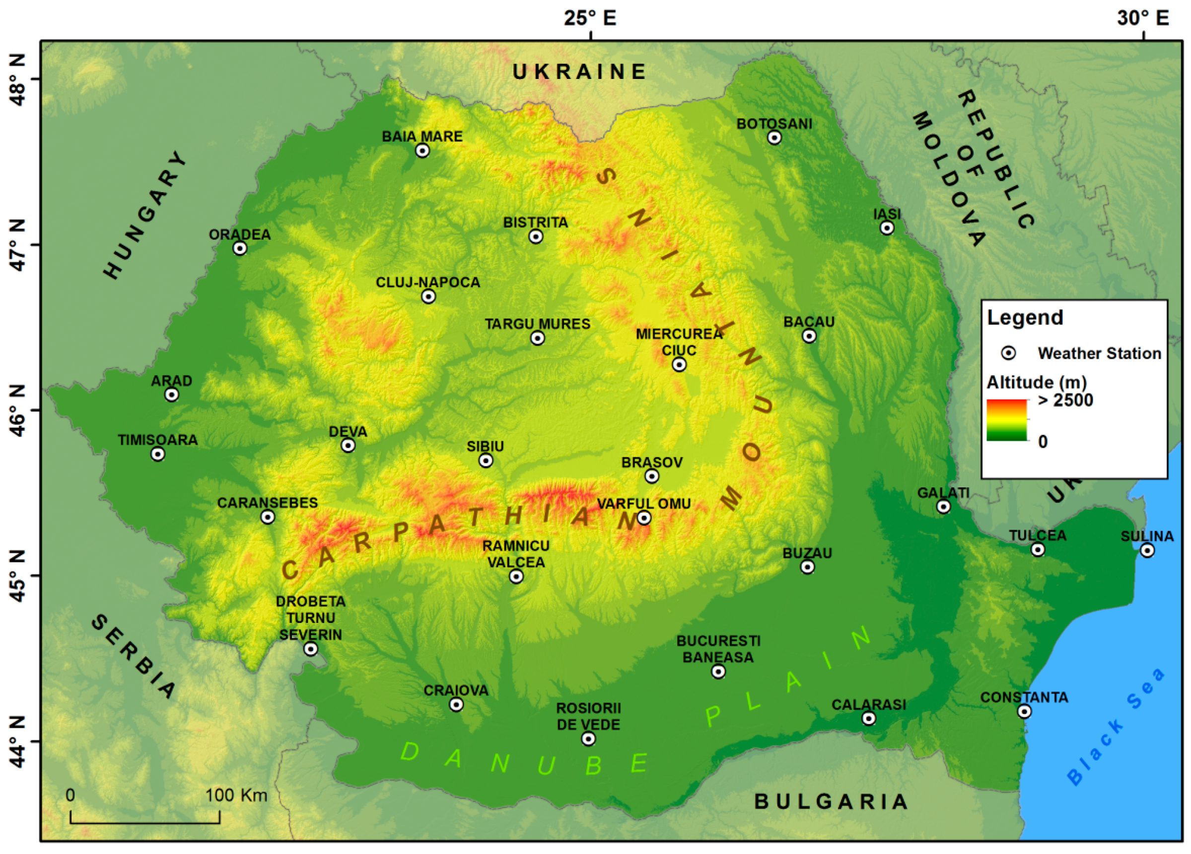
Figure 1. Location of weather stations used for this study.
Atmosphere 08 00050 g001
Figure 2. (a) Mean five-day backward trajectories of air particles before the first day of A1 HW/WS type; (b) composite sea level pressure anomaly; (c) composite air temperature anomaly at 850 hPa; and (d) composite of jet stream mean position anomaly at 300 hPa for A1 HW/WS type.
Atmosphere 08 00050 g002
Figure 3. (a) Mean five-day backward trajectories of air particles before the first day of A2 HW/WS type; (b) composite sea level pressure anomaly; (c) composite air temperature anomaly at 850 hPa; and (d) composite jet stream mean position anomaly at 300 hPa for A2 HW/WS type.
Atmosphere 08 00050 g003
Figure 4. (a) Mean five-day backward trajectories of air particles before the first day of B1 HW/WS type; (b) composite sea level pressure anomaly; (c) composite air temperature anomaly at 850 hPa; and (d) composite jet stream mean position anomaly at 300 hPa for B1 HW/WS type.
Atmosphere 08 00050 g004
Figure 5. (a) Mean five-day backward trajectories of air particles before the first day of B2 HW/WS type; (b) composite sea level pressure anomaly; (c) composite air temperature anomaly at 850 hPa; and (d) composite jet stream mean position anomaly at 300 hPa for B2 HW/WS type.
Atmosphere 08 00050 g005
Figure 6. (a) Mean five-day backward trajectories of air particles before the first day of B3 HW/WS type; (b) composite sea level pressure anomaly; (c) composite air temperature anomaly at 850 hPa; and (d) composite jet stream mean position anomaly at 300 hPa for B3 HW/WS type.
Atmosphere 08 00050 g006
Figure 7. Five-year frequency of HWs/WSs days in Romania (1961–2015) during: (a) radiative sub-types; and (b) advective sub-types.
Atmosphere 08 00050 g007
Figure 8. Absolute monthly frequency of HWs/WSs days in Romania (1961-2015) during (a) radiative sub-types; and (b) advective sub-types.
Atmosphere 08 00050 g008
Figure 9. Mean maximum temperature anomaly in Romania in summer (a); and mean maximum temperature in: June (b); July (c); and August (d) for A1 HW type based on ROmanian ClimAtic DAtaset (ROCADA) gridded database.
Atmosphere 08 00050 g009
Figure 10. Mean maximum temperature anomaly in Romania in summer (a); and mean maximum temperature in: June (b); July (c); and August (d) for A2 HW type based on ROCADA gridded database.
Atmosphere 08 00050 g010
Figure 11. Mean maximum temperature anomaly in Romania in spring and autumn (a); and mean maximum temperature in: March/November (b); April/October (c); and May/September (d), for B1 HW/WS type based on the ROCADA gridded database.
Atmosphere 08 00050 g011
Figure 12. Mean maximum temperature anomaly in Romania in spring and autumn (a); and mean maximum temperature in: March/November (b); April/October (c); and May/September (d), for B2 HW/WS type based on the ROCADA gridded database.
Atmosphere 08 00050 g012
Figure 13. Mean maximum temperature anomaly in Romania in winter (a); and mean maximum temperature in: December (b); January (c); and February (d) for B3 WS type based on the ROCADA gridded database.
Atmosphere 08 00050 g013
Table 1. Geographical coordinates of the weather stations considered.
No.Station Name *Latitude (N)Longitude (E)Altitude (m)Missing Daily Data (%)
Western Romania
1.Oradea47°02′10″21°53′51”1360.0
2.Arad46°08′15″21°21′13″1170.0
3.Timisoara45°46′17″21°15′35″860.0
4.Caransebes45°25′01″22°13′30″2410.0
Eastern Romania
5.Botosani47°44′08″26°38′40″1610.0
6.Bacau46°31′54″26°54′45″1840.0
7.Iasi47°10′15″27°37′42″1020.0
8.Galati45°28′23″28°01′56″710.0
Southern Romania
9.Buzau45°07′57″26°51′05″970.0
10.Ramnicu Valcea45°05′19″24°22′45″2390.5
11.Drobeta-Turnu Severin44°37′43″22°37′33″770.3
12.Bucuresti Baneasa44°31′00″26°05′00″900.0
13.Craiova44°18′36″23°52′00″1920.0
14.Calarasi44°12′22″27°20′18″190.0
15.Rosiori de Vede44°06′26″24°58′42″1020.0
Central Romania
16.Bistrita47°08′56″24°30′49″3670.0
17.Cluj-Napoca46°46′39″23°34′17″4100.0
18.Targu Mures46°32′01″24°32′07″3170.0
19.Deva45°51′52″22°53′55″2300.0
20.Sibiu45°47′21″24°05′28″4440.0
21.Brasov45°41′46″25°31′40″5350.0
Southwestern Romania
22.Tulcea45°11′26″28°49′26″40.1
23.Sulina45°02′26″23°16′35″30.2
24.Constanta44°12′49″28°38′41″130.0
Carpathians region
25.Baia Mare47°39′40″23°29′36″2240.0
26.Miercurea Ciuc46°22′16″25°46′21″6610.0
27.Varful Omu45°26′45″25°27′24″25040.0
* Weather stations are ordered from North to South for each region.

