
The Influence of an Increase of the Mediterranean Sea Surface Temperature on Two Nocturnal Offshore Rainbands: A Numerical Experiment


Abstract
:1. Introduction
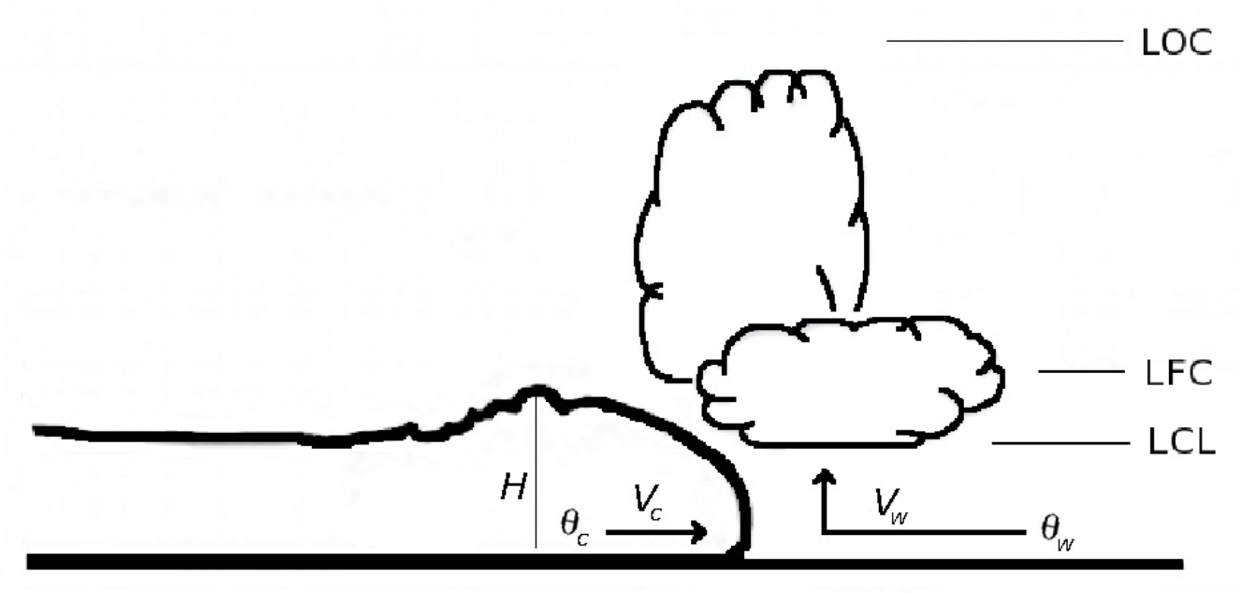
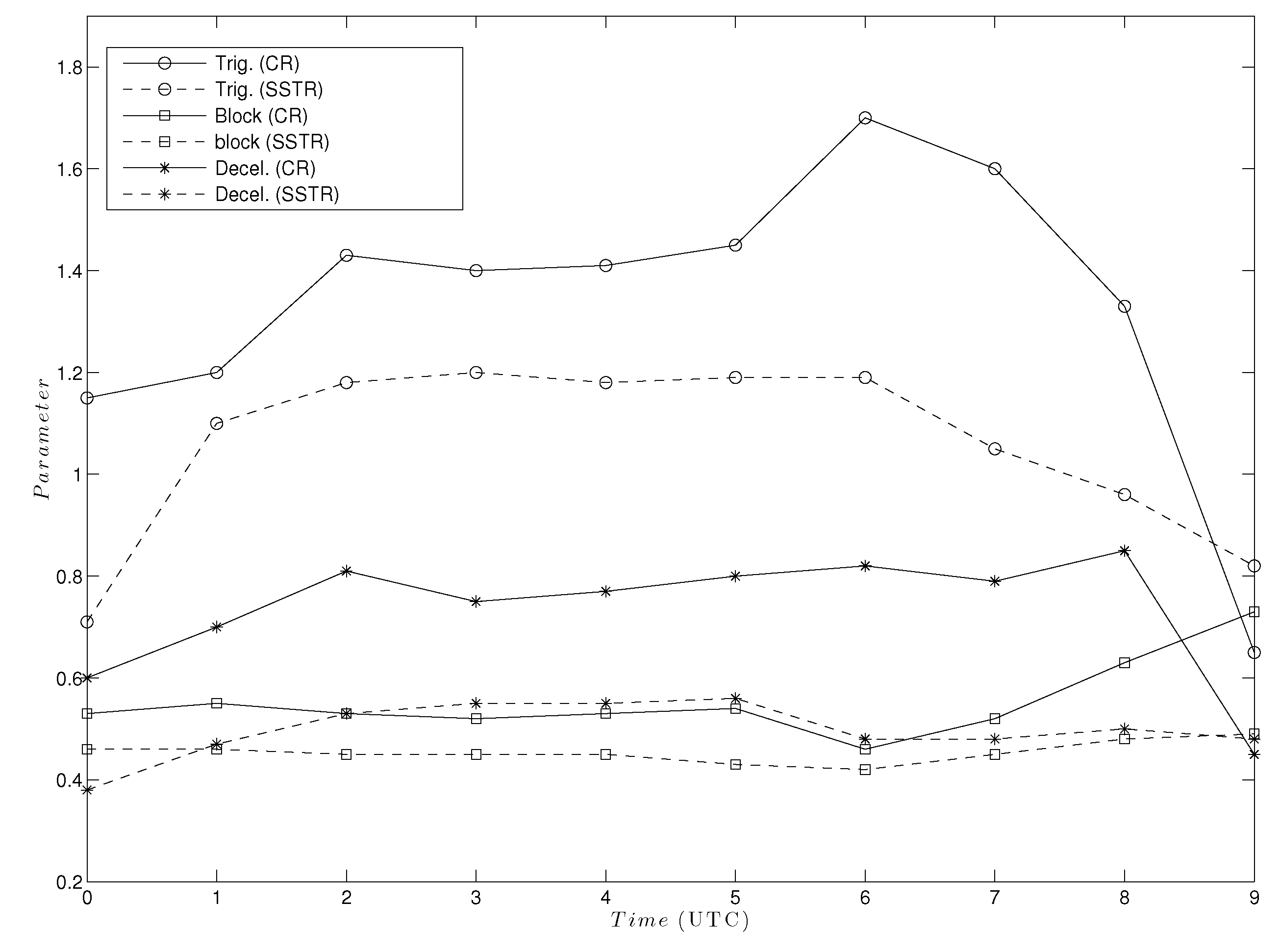
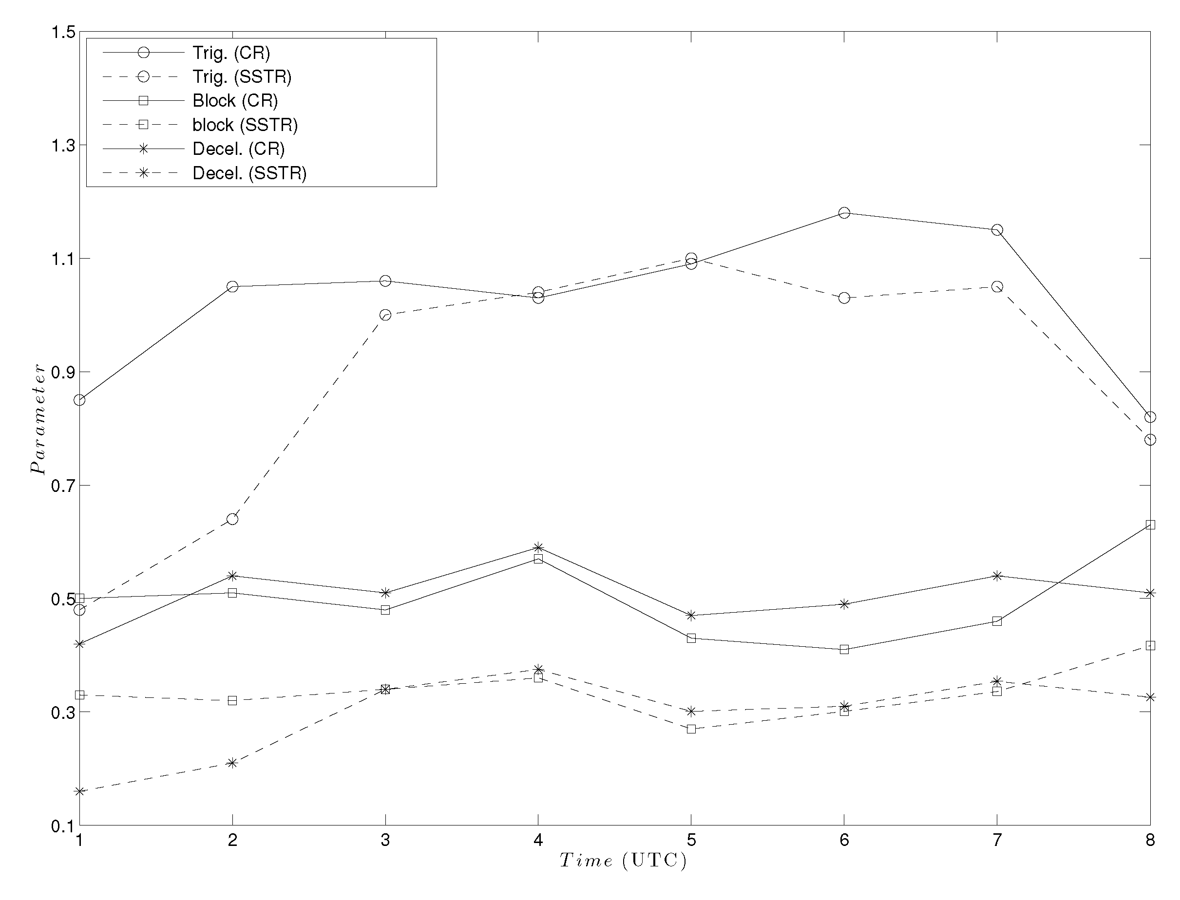
1.1. Theoretical Parameters
1.2. SST on the Mediterranean Basin
2. Methodology
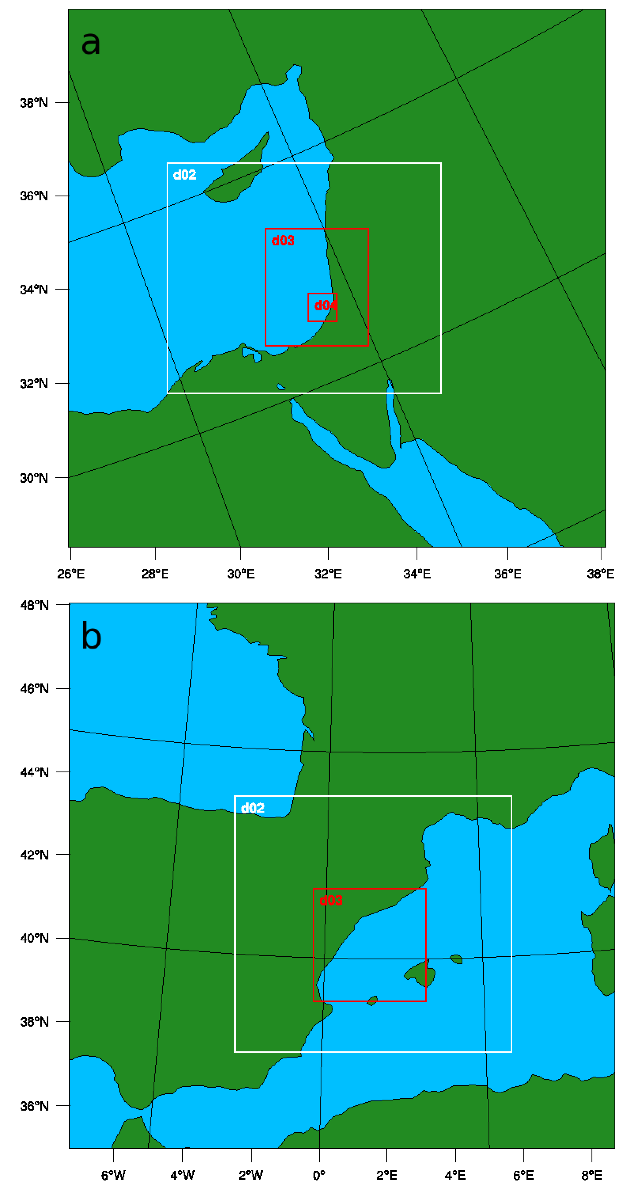
WRF Set-Up
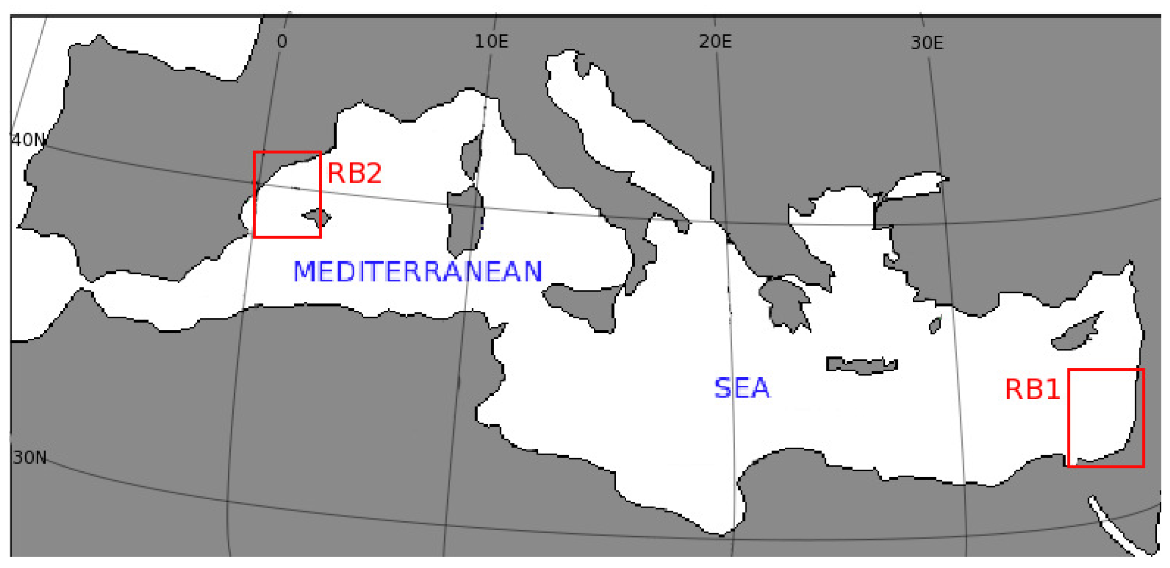
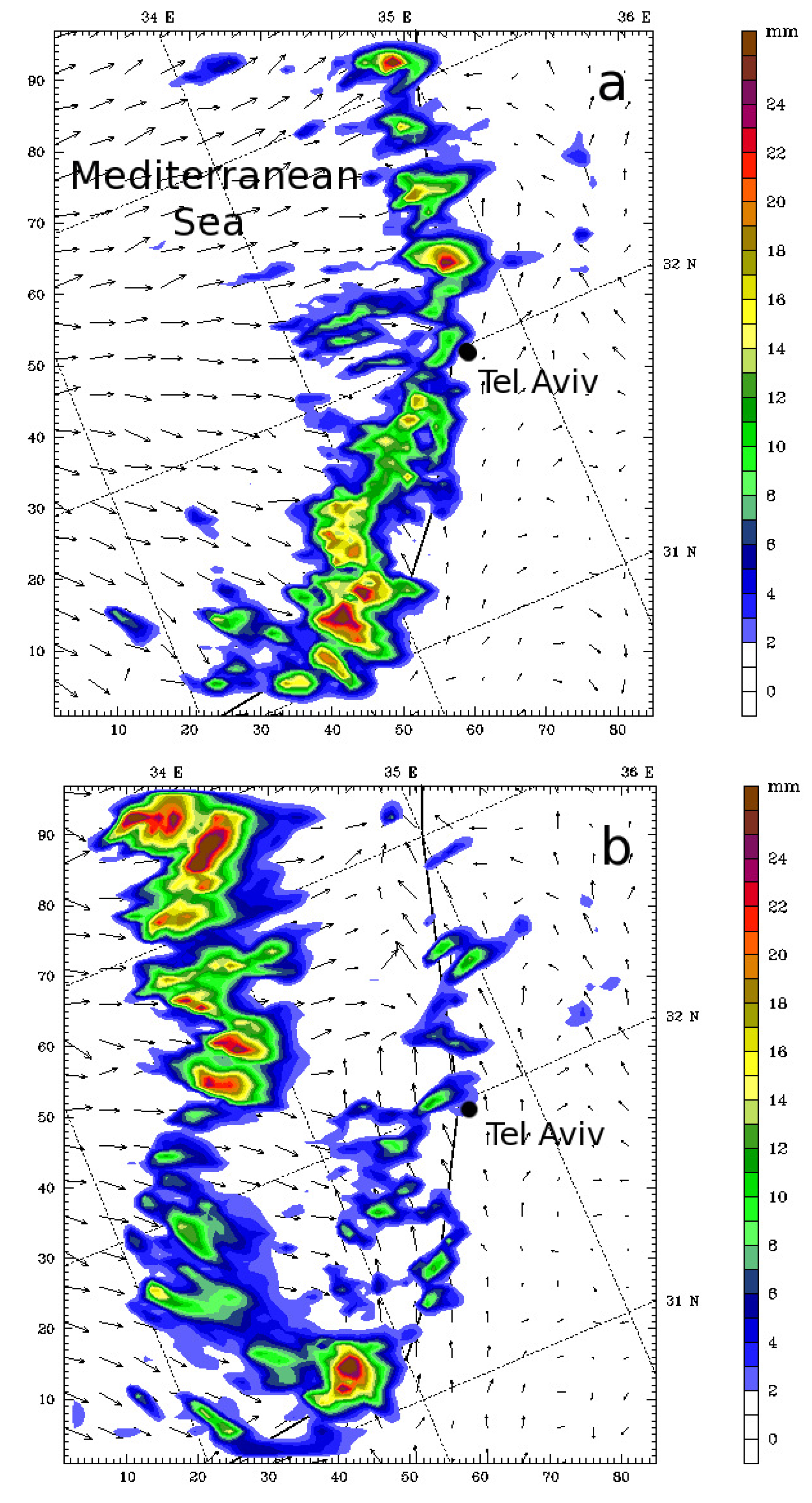
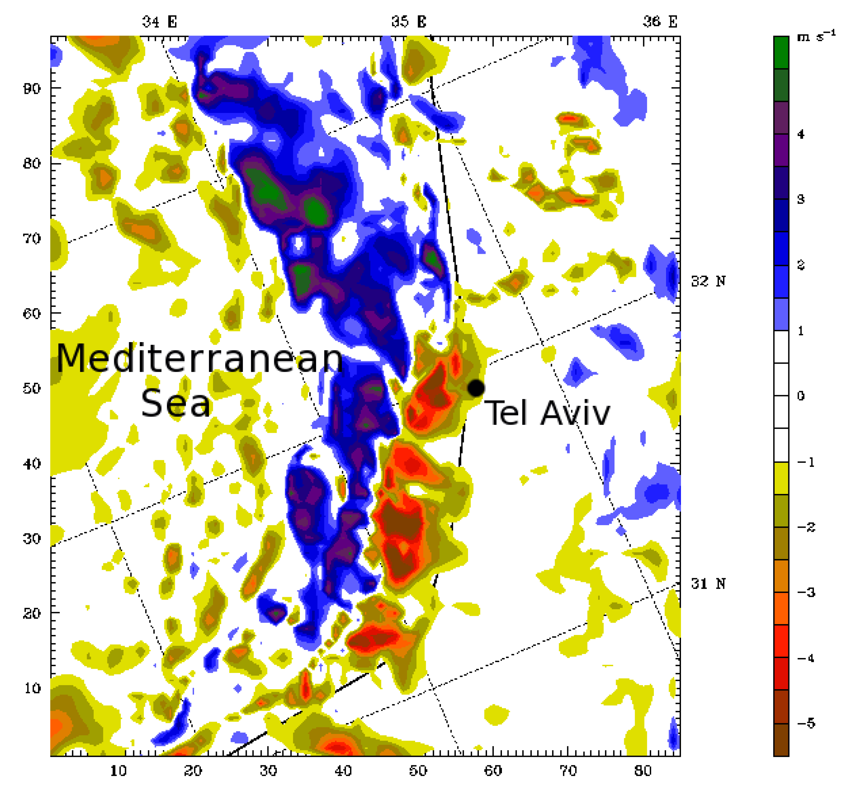
3. The Rainband in the Eastern Mediteranean Basin: RB1
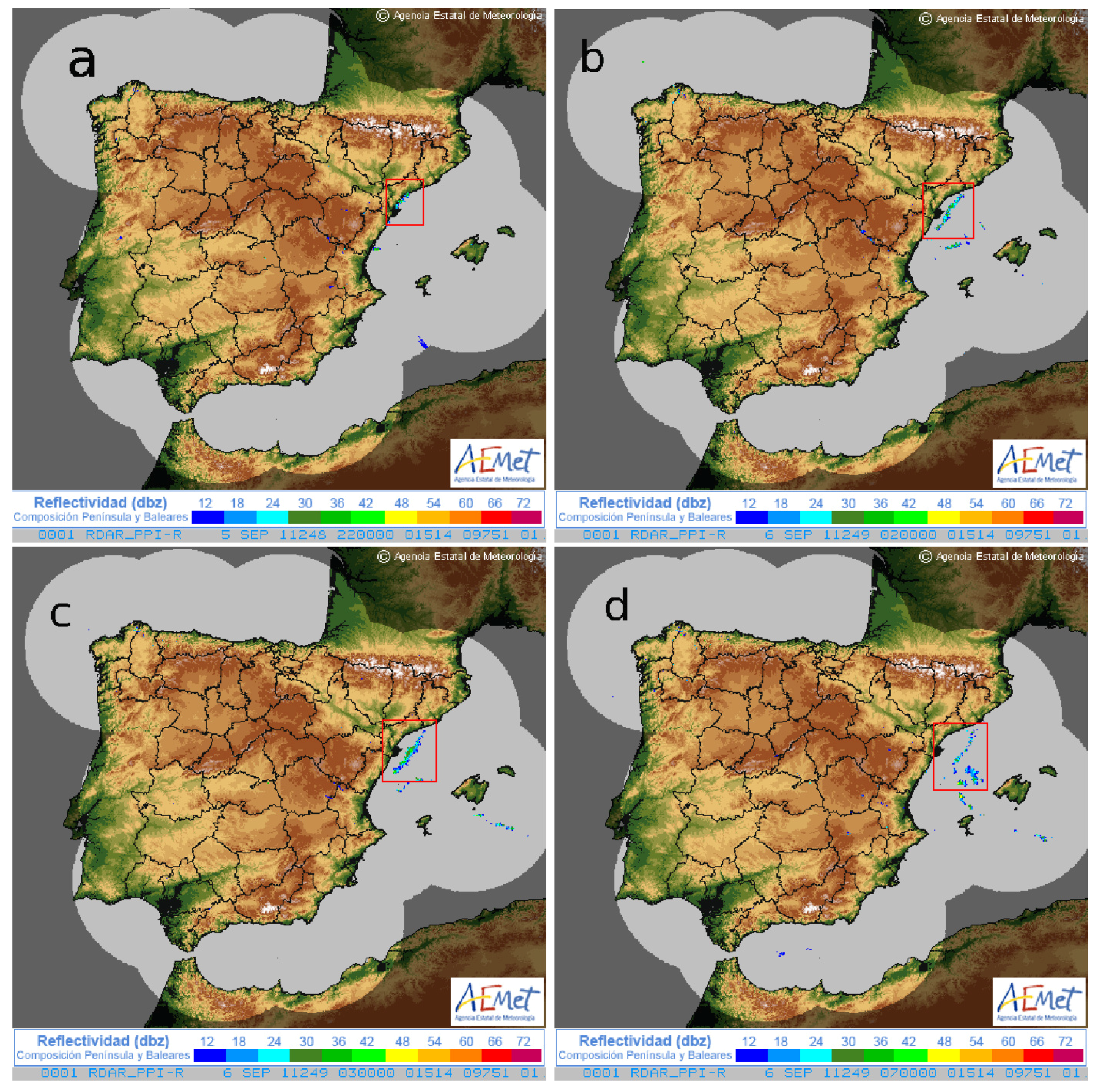
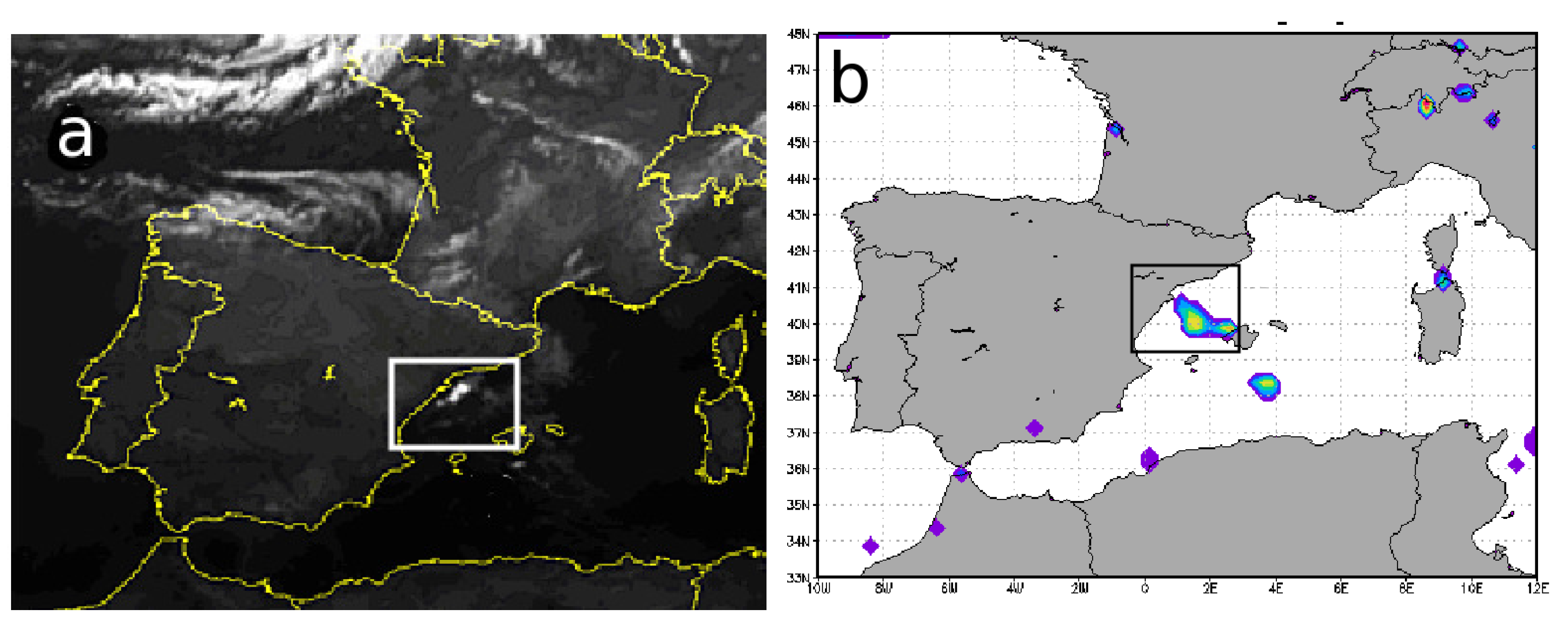
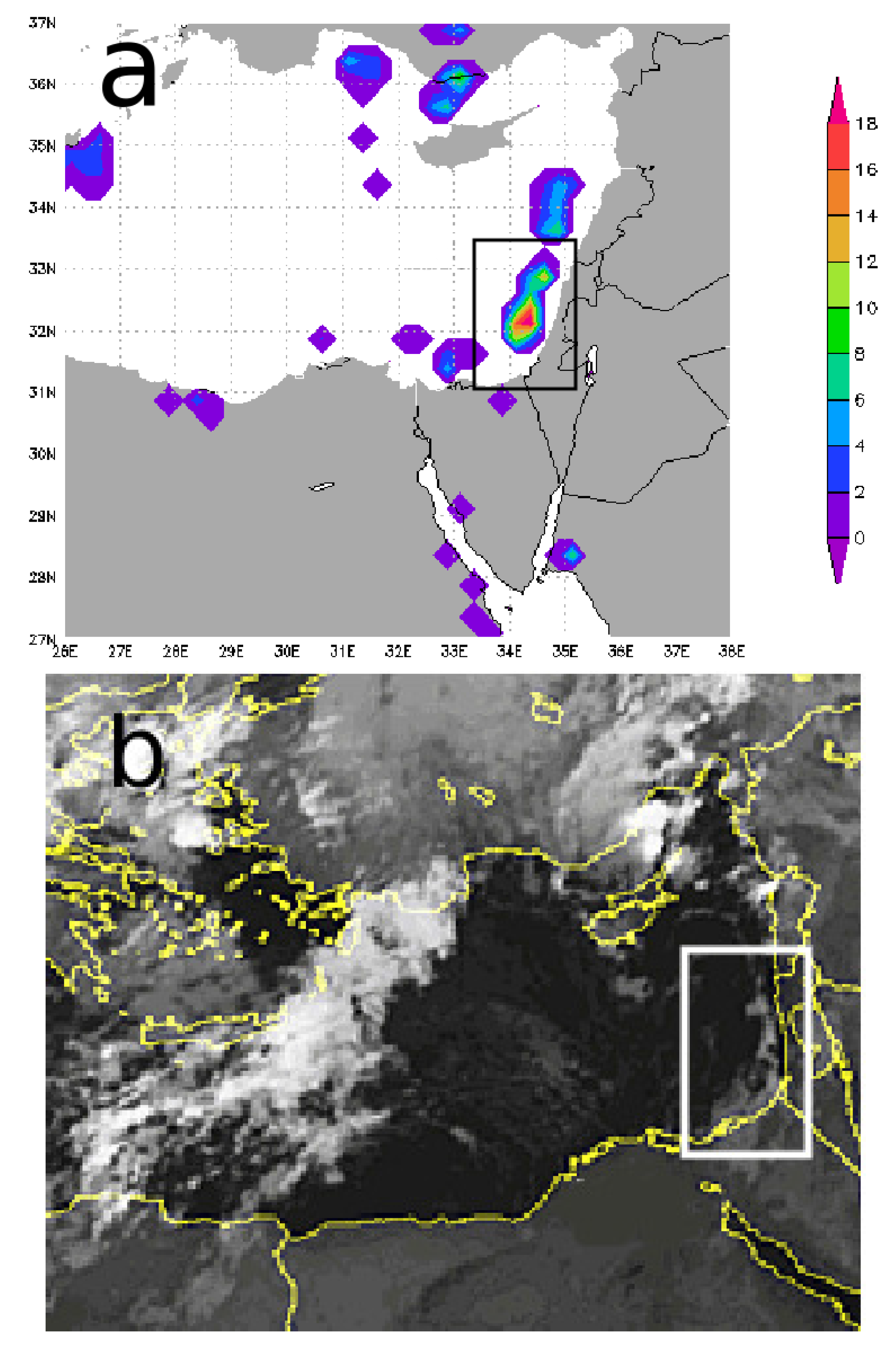
3.1. Observations
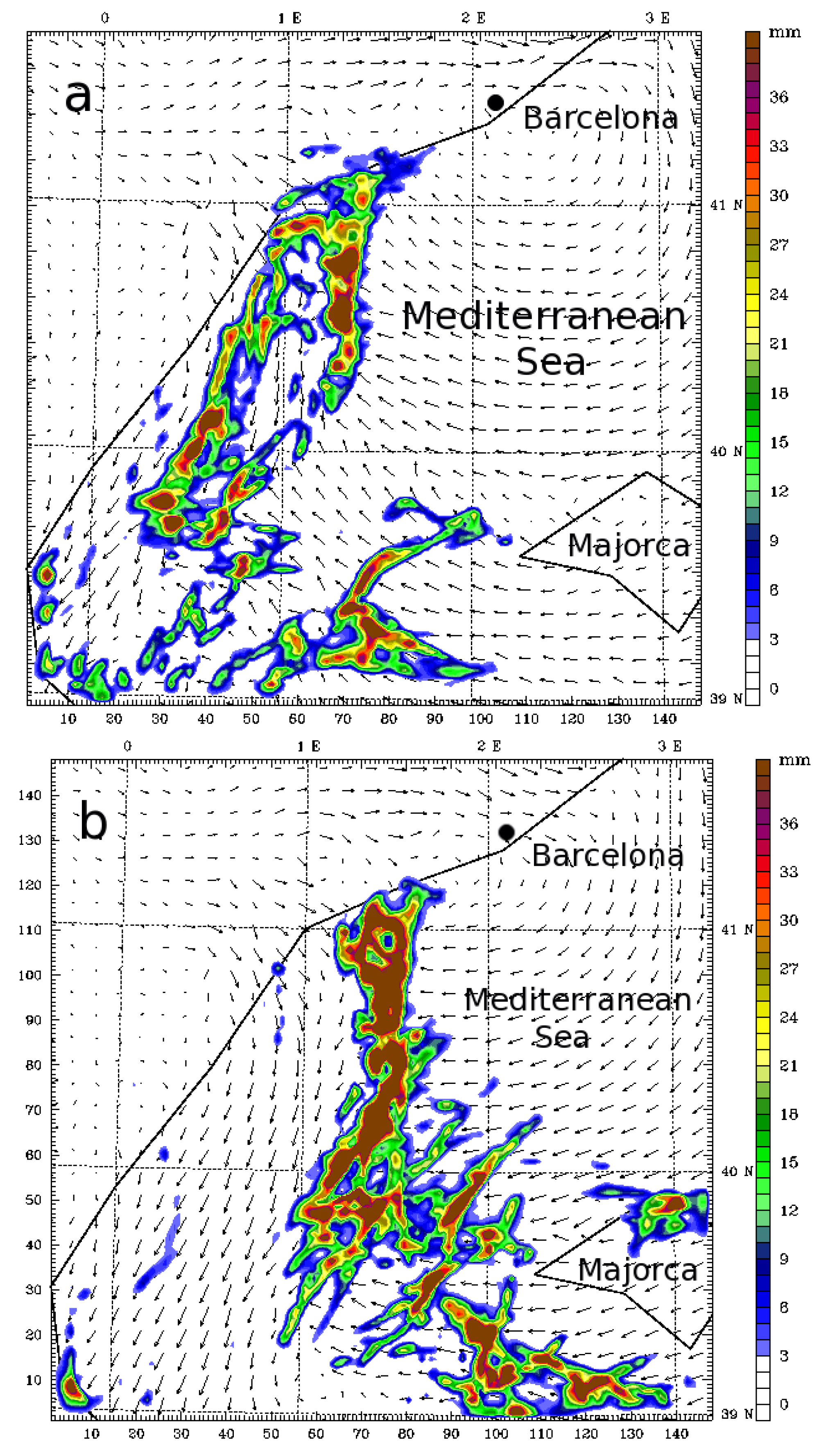
3.2. Numerical Simulations
4. The Rainband in the Western Mediterranean Basin: RB2
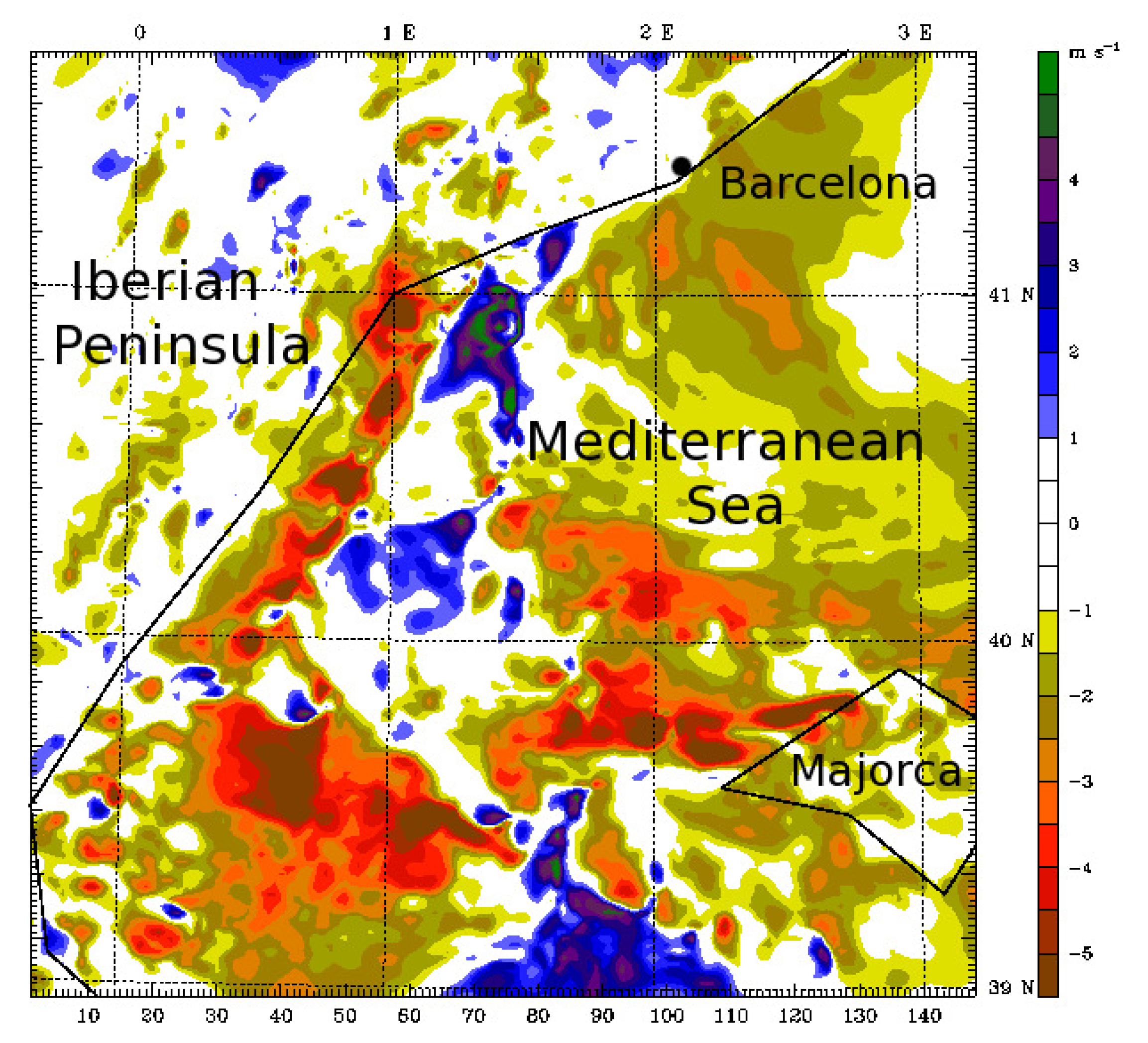
4.1. Observations
4.2. Numerical Simulations
5. Conclusions
Acknowledgments
Author Contributions
Conflicts of Interest
References
- Wang, J.J.; Rauber, R.; Ochs, H.T.I.; Carbone, R.E. The effects of the island of Hawaii on offshore rainband evolution. Mon. Weather Rev. 2000, 128, 1052–1069. [Google Scholar] [CrossRef]
- Ohsawa, T.; Ueda, H.; Hayashi, T.; Watanabe, A.; Masumoto, J. Diurnal variations of convective activity and rainfall in tropical Asia. J. Meteorol. Soc. Jpn. 2003, 79, 333–352. [Google Scholar] [CrossRef]
- Mapes, B.; Warner, T.; Xu, M.; Negri, A. Diurnal patterns of rainfall in northwestern South America. Part III: Diurnal gravity waves and nocturnal convection offshore. Mon. Weather Rev. 2003, 131, 830–884. [Google Scholar] [CrossRef]
- Yu, C.K.; Jou, B.J. Radar observations of the diurnal forced offshore convection lines among the southeastern coast of Taiwan. Mon. Weather Rev. 2004, 133, 1613–1636. [Google Scholar] [CrossRef]
- Neumann, J. Land breezes and nocturnal thunderstorms. J. Meteorol. 1951, 8, 60–67. [Google Scholar] [CrossRef]
- Greich, Y.; Mozes, H.; Rosenfeld, D. Radar analysis of cloud systems and their rainfall yield in Israel. Isr. J. Earth Sci. 2004, 53, 63–76. [Google Scholar]
- Mazon, J.; Pino, D. The role of nocturnal Low–Level–Jet in nocturnal convection and rainfalls in the west Mediterranean coast: The episode of 14 December 2010 in northeast of Iberian Peninsula. Adv. Sci. Res. 2011, 8, 27–31. [Google Scholar] [CrossRef] [Green Version]
- Mazon, J.; Pino, D. Numerical simulation of relatively heavy nocturnal rainbands associated with nocturnal coastal fronts in the Mediterranean basin. Nat. Hazards Earth Syst. Sci. Discuss 2013, 1, 7595–7613. [Google Scholar] [CrossRef]
- Mazon, J.; Pino, D. Role of the nocturnal coastal–front depth on cloud formation and precipitacion in the Mediterranean basin. Atmos. Res. 2015, 153, 145–154. [Google Scholar] [CrossRef]
- Schoenberg, L.M. Doppler radar observation of land–breeze cold front. Geophys. Res. Lett. 1984, 112, 2455–2464. [Google Scholar]
- Miglietta, M.; Rotunno, R. Numerical simulations of low–CAPE flows over a mountain ridge. J. Atmos. Sci. 2010, 67, 2391–2401. [Google Scholar] [CrossRef]
- Meyer, J.H. Radar observations of land breeze fronts. J. Appl. Meteorol. 1971, 10, 1224–1232. [Google Scholar] [CrossRef]
- Heiblum, R.H.; Koren, I.; Altaratz, O. Coastal precipitation formation and discharge based on TRMM observations. Atmos. Chem. Phys. 2011, 11, 13201–13217. [Google Scholar] [CrossRef]
- Mapes, B.; Warner, T.; Xu, M.; Negri, A. Diurnal patterns of rainfall in northwestern South America. Part I: Observations and context. Mon. Weather Rev. 2003, 131, 799–812. [Google Scholar] [CrossRef]
- Malda, D.; Vilà-Guerau de Arellano, J.; van der Berg, W.D.; Zuurendonk, I.W. The role of atmospheric boundary layer-surface interactions on the development of coastal fronts. Ann. Geophys. 2007, 25, 341–360. [Google Scholar] [CrossRef]
- Lin, Y.L.; Chiao, S.; Wang, T.A.; Kaplan, M.; Weglarz, R. Some common ingredients for heavy orographic rainfall. Weather Forecast. 2001, 16, 633–660. [Google Scholar] [CrossRef]
- Durran, D.R.; Klemp, J.B. Another look at down–slope winds. Part II: Nonlinear amplification beneath wave–overturning layers. J. Atmos. Sci. 1987, 44, 3402–3412. [Google Scholar] [CrossRef]
- Simpson, J.E.; Britter, R.E. A laboratory model of atmospheric mesofront. Q. J. R. Meteorol. Soc. 1980, 106, 485–500. [Google Scholar] [CrossRef]
- Miglietta, M.; Moscatello, A.; Conte, D.; Mannarini, G.; Lacarata, G.; Rotunno, R. Numerical analysis of a Mediterranean hurricane over south-eastern Italy: Sensitivity experiments to sea surface temperature. Atmos. Res. 2011, 101, 412–426. [Google Scholar] [CrossRef]
- Senatore, A.; Mendicino, G.; Knoche, H.-R.; Kunstmann, H. Sensitivity of modeled precipitation to sea surface temperature in regions with complex topography and coastlines: A case study for the Mediterranean. J. Hydrometeorol. 2014, 15, 2370–2396. [Google Scholar] [CrossRef]
- Kavvada, A.; Ruiz-Barradas, A.; Nigam, S. Climate Change 2013: The Physical Science Basis. Contribution of Working Group I to the Fifth Assessmant Report of the Interguvernamental Panel on Climate Change; Technical Report; Cambrige University Press: Cambrige, UK, 2013. [Google Scholar]
- Trenberth, K.E.; Jones, P.H.; Ambenje, P.; Bojariu, R.; Easterling, D.; Tank, A.K.; Parker, D.; Rahimzadeh, F.; Renwick, J.A.; Rusticucci, M.; et al. Climate Change 2007: The Physical Science Basis. Contribution of Working Group I to the Fourth Assessment Report of the Intergovernmental Panel on Climate Change; Chapter 3. Observations: Surface and Atmospheric Climate Change; Solomon, S., Qin, D., Manning, M., Chen, Z., Marquis, M., Averyt, K.B., Tignor, M., Miller, H.L., Eds.; Cambridge University Press: Cambridge, UK, 2007. [Google Scholar]
- Rixen, M.; Beckers, J.; Levitus, S.; Antonov, J.; Boyer, T.; Maillard, C.; Fichaut, M.; Balopoulos, E.; Iona, S.; Dooley, H.; et al. The Western Mediterranean deep water: A proxy for climate change. Geophys. Res. Lett. 2005, 32. [Google Scholar] [CrossRef]
- Vargas-Yáñez, M.; García, M.J.; Salat, J.; García-Martínez, M.C.; Pascual, J.; Moya, F. Warming trends and decadal variability in the Western Mediterranean shelf. Glob. Planet. Chang. 2008, 63, 177–184. [Google Scholar] [CrossRef]
- Salat, J.; Pascual, J. The oceanographic and meteorological station at l’Estartit (NW Mediterranean). In Tracking Long-Term Hydrographical Change in the Mediterranean Sea; CIESM Workshop Series; CIESM: Madrid, Spain, 2002; pp. 29–32. [Google Scholar]
- Salat, J.; Pascual, J. Principales Tendencias Climatológicas en el Mediterráneo Noroccidental, a Partir de más de 30 años de Observaciones Oceanográficas en la Costa Catalana; Clima, Sociedad y Medio Ambiente; Asociación Española de Climatología: Madrid, Spain, 2006; Volume Serie A, pp. 284–290. [Google Scholar]
- Somot, S.; Sevault, F.; Déqué, M.; Crépon, M. 21st century climate change scenario for the Mediterranean using a coupled atmosphere–ocean regional climate model. Glob. Planet. Chang. 2008, 63, 112–126. [Google Scholar] [CrossRef]
- Kavvada, A.; Ruiz-Barradas, A.; Nigam, S. AMOs structure and climate footprint in observations and IPCC AR5 climate simulations. Clim. Dyn. 2013, 41, 1345–1364. [Google Scholar] [CrossRef]
- Williams, E. Global circuit response to seasonal variations in global surface air temperature. Mon. Weather Rev. 1994, 117, 1917–1929. [Google Scholar] [CrossRef]
- Ye, B.; del Genio, A.; Lo, K.K.W. CAPE variations in the current climate and in a climate change. J. Clim. 1998, 11, 2985–3002. [Google Scholar] [CrossRef]
- Skamarock, W.C.; Klemp, J.B.; Dudhia, J.; Gill, D.O.; Barker, D.M.; Duda, M.; Huang, X.Y.; Wan, W.; Powers, J.G. A Description of the Advanced Research WRF Version 3; Technical Report TN–475+STR; NCAR: Boulder, CO, USA, 2008. [Google Scholar]
- Hong, S.Y.; Pan, H.L. Nonlocal boundary layer vertical diffusion in a medium-range forecast model. Mon. Weather Rev. 1996, 124, 2322–2339. [Google Scholar] [CrossRef]
- Mlawer, E.J.; Taubman, S.J.; Brown, P.D.; Iacono, M.J.; Clough, S.A. Radiative transfer for inhomogeneous atmospheres: RRTM, a validated correlated–k model for the longwave. J. Geophys. Res. 1997, 102, 663–682. [Google Scholar] [CrossRef]
- Dudhia, J. Numerical study of convection observed during the winter monsoon experiment using a mesoscale two–dimensional model. J. Atmos. Sci. 1989, 46, 3077–3107. [Google Scholar] [CrossRef]
- Hong, S.H.; Dudhia, J.; Chen, S.H. A revised approach to ice microphysical processes for the bulk parameterization of clouds and precipitation. Mon. Weather Rev. 2004, 132, 103–120. [Google Scholar] [CrossRef]
- Kain, J. The Kain–Fritsch convective parameterization: An update. J. Appl. Meteorol. 2004, 43, 170–181. [Google Scholar] [CrossRef]
- Haddad, Z.S.; Smith, E.A.; Kummerow, C.D.; Iguchi, T.; Farrar, M.R.; Durnen, S.L.; Alves, M.; Olson, W.S. The TRMM ’day–1’ radar/radiometer combined rain profiling algorithm. J. Meteorol. Soc. Jpn. 1997, 75, 799–809. [Google Scholar]
- Khain, A.P.; Rosenfeld, D.; Sednev, I.L. Coastal effects in the Eastern Mediterranean as seen from experiments using a cloud ensemble model with a detailed description of warm and ice microphysical processes. Atmos. Res. 1993, 30, 295–319. [Google Scholar] [CrossRef]


© 2017 by the authors. Licensee MDPI, Basel, Switzerland. This article is an open access article distributed under the terms and conditions of the Creative Commons Attribution (CC BY) license ( http://creativecommons.org/licenses/by/4.0/).
Share and Cite
Mazon, J.; Pino, D. The Influence of an Increase of the Mediterranean Sea Surface Temperature on Two Nocturnal Offshore Rainbands: A Numerical Experiment. Atmosphere 2017, 8, 58. https://doi.org/10.3390/atmos8030058
Mazon J, Pino D. The Influence of an Increase of the Mediterranean Sea Surface Temperature on Two Nocturnal Offshore Rainbands: A Numerical Experiment. Atmosphere. 2017; 8(3):58. https://doi.org/10.3390/atmos8030058
Chicago/Turabian StyleMazon, Jordi, and David Pino. 2017. "The Influence of an Increase of the Mediterranean Sea Surface Temperature on Two Nocturnal Offshore Rainbands: A Numerical Experiment" Atmosphere 8, no. 3: 58. https://doi.org/10.3390/atmos8030058
APA StyleMazon, J., & Pino, D. (2017). The Influence of an Increase of the Mediterranean Sea Surface Temperature on Two Nocturnal Offshore Rainbands: A Numerical Experiment. Atmosphere, 8(3), 58. https://doi.org/10.3390/atmos8030058