Atmospheric Volatile Organic Compounds in a Typical Urban Area of Beijing: Pollution Characterization, Health Risk Assessment and Source Apportionment

Abstract

Atmospheric volatile organic compounds (VOCs) measurement was carried out using gas chromatography-flame ionization detector (GC-FID) technique (Airmo VOCs online analyzer) in a typical urban area in Beijing from April 2014 to January 2015. Ambient levels, variation characteristics and influential factors contributing to the formation of near-ground-ozone and secondary organic aerosols as well as health risk assessment of VOCs were analyzed. Based on these analyses, the important VOC species that should be given more attention for pollution control were identified and the source apportionment of VOCs was made. Suggestions for VOCs pollution control countermeasures were put forward. The annual average concentration of 84 VOCs was 119 μg·m⁻³ and the hourly mean concentration was 9.11–567 μg·m⁻³. Ambient level of VOCs in Beijing has been alleviated in recent years, but is still severe compared to some other cities. VOCs with the largest proportion were alkanes in spring and halogenated hydrocarbons in summer, autumn and winter. The variation of 84 VOCs concentrations was consistent with that of the ambient air quality index, indicating that VOCs had a strong influence on ambient air quality. Influenced by the concentration and activity of VOCs, the largest contribution to ozone formation potential and secondary organic aerosol formation potential came from alkenes and aromatic hydrocarbons, respectively. Five VOCs species such as benzene pose carcinogenic risk to exposed populations. Contrary to some previous studies, benzene was found to have potential cancer risk in some urban areas in China. The main sources of VOCs in the study area were vehicle exhaust, solvent usage, and industrial processes. In order to improve air quality in Beijing and reduce the infection rate of air pollutant related diseases, it is necessary to strengthen the control the emission of VOCs from those three sources.

1. Introduction

The term “Volatile Organic Compounds (VOCs)” generally refers to a group of organic chemicals that have a high vapor pressure at room temperature conditions. At present, there is no globally accepted definition of atmospheric VOCs, although different definitions of VOCs have been developed by some international organizations and national institutions from various viewpoints [1]. WHO defines VOCs as volatile compounds in ambient air with a boiling point between 50 and 260 °C and saturated vapor pressure exceeding 133.322 Pa at room temperature (20 °C) [2]. VOCs can lead to photochemical smog pollution and promote the formation of haze. Some VOCs such as halocarbons consume ozone in the stratosphere and cause the formation of ozone holes. Some toxic VOCs, such as benzene, toluene and formaldehyde, are harmful to human health and have carcinogenic, teratogenic and mutagenic effects [3].

In recent years, with sustained and rapid development of China’s national economy, industrialization and urbanization have been accelerating and the number of vehicles has increased dramatically. Energy consumption has been so great that air pollution exceeds the environmental carrying capacity, with such pollution in cities and urban agglomerations. This is mainly manifested in the decline of atmospheric visibility and frequent occurrence of heavy pollution episodes. Regarding urban air quality, only 21.6% of 338 prefecture-level cities met the China Air Quality Standard in 2015. Beijing-Tianjin-Hebei, as one of the fastest growing areas in China, was also one of the heaviest air pollution regions. There were totally 1710 days of heavy pollution in Beijing, Tianjin, and Hebei provinces and 70 surrounding prefecture-level cities in 2015, constituting 44.1% of total heavy pollution days in China [4]. As the capital of China, Beijing is China’s political, economic, educational, cultural and international exchange center, and is representative of China’s international image. Recently, the annual concentration of pollutants generally decreased in Beijing. However, the annual average mass concentration of particulate matter 2.5 (PM_2.5) and NO₂ and maximum 8-h average 90th percentile concentration of ozone were 80.6, 50 and 202.6 μg·m⁻³ respectively, which are 1.3 (Grade 1 Limit value: 35), 0.25 (Grade 1 Limit value: 40) and 0.27 (Grade 2 Limit value: 160) times higher than relevant limits in the China Air Quality Standard [5]. The urban area of Beijing is an especially VOCs sensitive area and the generation of ozone is limited by VOCs [6,7,8,9,10], thus it is important to control the VOCs. Under such situation, as important precursors of fine atmospheric particles and surface ozone, VOCs should be controlled immediately. Atmospheric VOCs have not been included in the routine monitoring system, and there is a lack of comprehensive knowledge of the pollution characteristics of VOCs in the ambient air of Beijing. To develop effective VOCs control measures, it is very important to study those pollution characteristics.

Studies on VOCs in ambient air have mainly considered the pollution level, spatiotemporal variation, and atmospheric VOCs photochemical activity. There is a lack of research on risk assessment, source analysis, and gas-phase factors. Most studies in China used offline, short-term sampling and analysis technology, which did not meet the requirement of long-term and high-resolution research of ambient air [11]. Considering the importance of VOCs and the pollution status in Beijing, it is critical to carry out long-term and high-resolution monitoring of VOCs in the ambient air of Beijing and comprehensively analyze their pollution characteristics.

In this study, pollution levels, the composition and variation of 84 VOCs in ambient air and the impact of meteorological factors were analyzed using online monitoring data of VOCs in a typical urban area of Beijing, where observation period was selected from April 2014 to January 2015. The atmospheric photochemical reactivity of VOCs and contribution to the formation of ozone and secondary organic aerosols (SOAs) were studied. Risks of certain VOCs to human health were evaluated and the sources of 84 VOCs investigated. Based on the results, measures are proposed to control VOCs pollution in ambient air of urban areas in Beijing.

2. Materials and Methods

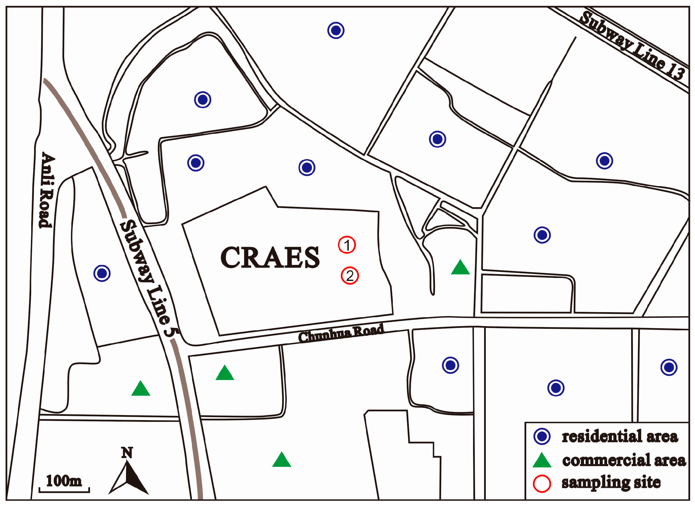
2.1. Monitoring Site and Period

The monitoring site was on the roof of the Atmospheric Photochemical Smog Simulation Laboratory of the Chinese Research Academy of Environmental Sciences (CRAES) (40.04° N, 116.42° E), in the Chaoyang District of Beijing. This was about 8 m above ground (Figure 1). The site was in a residential and commercial area, and there was no obvious pollution source nearby. This was a typical urban area to study VOCs pollution and its risk to human health in Beijing urban areas.

Since June 2013, VOCs in ambient air were continuously monitored using online VOCs monitoring equipment at the sampling site, and much valuable data were obtained. Considering the representation and validity of these data, 120 days of online VOCs data were selected to be studied from April 2014 to January 2015. These days were divided into four 30-day seasons: 8–13 April 2014, 21 April–4 May 2014 and 9–18 May 2014 were selected as spring; 24 July–22 August 2014 were selected as summer; 6 October–4 November 2014 were selected as autumn; and 25 December 2014–23 January 2015 were selected as winter. At the same site and time, concentrations of conventional pollutants were observed, such as O₃, CO, SO₂, NO₂ and PM_2.5. In summer, meteorological data and conventional pollutants were also monitored on the roof, 10 m from the online VOCs sampling site and 15 m above ground. The surrounding environment was similar to that of the VOCs monitoring site. The meteorological data included wind speed, wind direction, temperature, humidity, precipitation, atmospheric pressure, solar radiation and ultraviolet radiation.

2.2. Monitoring Instruments

In this study, the Airmo online VOCs analyzer (Chromatotec Group, Bordeaux, France) was used to monitor VOCs. The instrument consists of air sampling, pollutant measurement, calibration and data acquisition units. It includes low-carbon (C₂–C₆) and high-carbon (C₆–C₁₂) analyzers. There are flame ionization detectors (FID), time resolution is 30 min, the minimum detectable limit is ppt-level, and the measurement range is 0.1–100 ppb. The instrument can qualitatively and quantitatively analyze 84 VOCs in ambient air, including 26 alkanes, 15 alkenes, 1 alkyne, 17 aromatic hydrocarbons, and 25 halogenated hydrocarbons. For specific halogenated hydrocarbons, the better choice is an Electron Capture Detector (ECD), which has higher sensitivity to negative electrons compared with FID. Some compounds could only be detected using ECD rather than FID. Considering the accuracy, the analysis of halogenated hydrocarbon was carried out very simply without further study.

The conventional pollutants were monitored by a model 49i O₃ analyzer, model 48i CO analyzer, model 43i SO₂ analyzer, model 17i NO₂ analyzer, and model 5030 sharp PM_2.5 monitor (Thermo Scientific Company, Waltham, MA, USA), in spring, autumn and winter. The aforementioned instruments were used in field monitoring and were unavailable for monitoring conventional pollutants in summer [12]. Therefore, EC9810B O₃, EC9850B SO₂, EC9830B CO and EC9841T NO₂ (ECOTECH Company, Melbourne, Australia), and BAM-1020 PM_2.5 (METONE Company, Grants Pass, WA, USA) analyzers were used to monitor the conventional pollutants in summer. Concentrations of organic carbon (OC) and elemental carbon (EC) in atmospheric aerosol were measured by a Model-4 automatic semi-continuous carbon analyzer (Sunset Laboratory Company, Tigard, OR, USA). The working principle of this instrument is photo-thermal absorption. Its time resolution is 60 min, and the measurement range is 0.2–1000 μgC·m⁻³ (online continuous monitoring).

The meteorological data were monitored by a Vaisala MAWS301 (Helsinki, Finland) automatic weather station. The instrument can simultaneously measure meteorological parameters such as wind speed, wind direction, temperature, humidity, air pressure, solar radiation, and ultraviolet radiation. Because this instrument was maintained in spring, the meteorological data in that season were from Beijing Capital International Airport [13]. There were no data of solar or ultraviolet radiation during this period.

2.3. Quality Assurance and Control

The Airmo analyzer was placed on the second floor of the Atmospheric Photochemical Smog Simulation Laboratory; the sampling port was installed on the roof of the building, and Airmo analyzer connected the sampling port through a sampling pipe and sampled ambient air. Air conditioning was used indoors. A sample tube was wrapped with a heating jacket and thermal insulation cover to ensure that the analyzer was running at 18–22 °C. To ensure the reliability of the observed data, the instrument was calibrated periodically during the observation period, by internal and external calibration. Internal calibration materials were n-butane, n-hexane and benzene, and the external one was a standard gas of VOCs complying with Photochemical Assessment Monitoring Stations (PAMS) and Compendium of Methods for the determination of toxic organic compounds in ambient air (TO-14) standard from US EPA [14,15]. The instrument was calibrated twice every 24 h internally and once every half year externally. Retention time, peak areas and concentration analysis curves could be viewed in the analyzer supporting software to clearly track the data.

The 49i O₃ and EC9810B O₃ analyzers were calibrated annually using Stand Reference Photometer (SRP) calibration from the Institute for Environmental Reference Materials of the China Ministry of Environmental Protection. Analyzers for other conventional pollutants were calibrated monthly using reference materials [16].

OC and EC in atmospheric aerosols were measured using a Model-4 automatic semi-continuous carbon analyzer (Sunset Laboratory Company). The instrument was calibrated by a normalized internal standard method. At the end of each analysis, the system automatically injected a fixed amount of standard gas to normalize the analysis result using the external standard gas. The calibration method automatically compensated changes in instrument drift and external conditions to ensure data accuracy.

2.4. Data Processing

During the study period, 84 VOCs were detected by the online VOCs analyzer, of which 12 were below the lower limit of the instrument and their concentrations were not obtained. However, all 84 VOCs were analyzed, and their concentrations expressed by ${\displaystyle \sum }84 \mathrm{VOCs}$.

Invalid mass concentration data of VOCs should be removed based on the internal calibration data. In our study, all observed data were within a reasonable range, except that some of the halogenated hydrocarbons did not have the available data, so there was no need to remove any data. During the monitoring, the instrument was calibrated internally twice a day, at 00:00 and 2:00. These two internal calibration data were removed automatically by the instrument, so there was one dataset at 00:00 and 2:00 in each time and two dataset from all other hours [17]. We obtained 463,680 valid data during the study period. Hourly average value for each species was calculated by taking the meaning value of 30-min values; for the internal calibration, the values in 00:00 and 2:00 were used to be hourly average value directly. Since two data of 30 min in each 60 min were usually about ±10% difference, we used one 30-min data to represent the data for 0:00 and 2:00. Based on those values, the trend, pollution characteristics and reactivity of VOCs were calculated and the health risks of certain species were evaluated. The observation periods were divided into daytime (6:00 to 18:00) and night (18:00 to 6:00) in the whole period (Chinese Standard Time). The days were separated into working and non-working days in accord with Chinese statutory holidays.

In spring 2014, a total of 240 OC and EC data were obtained. In summer, autumn and winter, 720 OC and EC data were acquired. The minimum value of OC/EC ((OC/EC)_min) of each season was taken into the corresponding equation to estimate secondary organic aerosol (SOA) values.

2.4.1. Calculation of Ozone Formation Potential of VOCs

In this study, maximum incremental reactivity (MIR) was used to analyze and evaluate the contribution of each VOCs to the formation of ozone.

The OFP of VOCs was calculated by

OFP = MIR × ρ (C₂–C₁₂)

(1)

where OFP is the ozone formation potential; MIR is the maximum incremental reactivity; ρ (C₂–C₁₂) is the mass concentration of VOCs; and MIR is the result from Atkinson et al. [18,19]. In the present study, 26 alkanes, 13 alkenes and 12 aromatic hydrocarbons (marked by “*” in

Table 1. Ambient levels of 84 VOCs and conventional pollutants (daily average ± standard deviation) (μg·m⁻³).

Species	Spring (n = 30)	Summer (n = 30)	Autumn (n = 30)	Winter (n = 30)	Annual
Alkanes
ethane *	3.68 ± 1.05	2.97 ± 0.84	6.36 ± 3.00	8.60 ± 4.33	5.40 ± 3.50
propane *	4.96 ± 1.84	5.70 ± 2.08	10.8 ± 5.8	12.2 ± 6.2	8.42 ± 5.40
i-butane *	2.36 ± 0.84	2.68 ± 0.66	4.06 ± 2.13	3.30 ± 1.85	3.10 ± 1.62
n-butane *	3.81 ± 1.28	3.64 ± 1.41	5.62 ± 3.56	5.58 ± 3.00	4.66 ± 2.66
cyclopentane *	3.22 ± 1.37	2.29 ± 1.72	4.35 ± 3.32	2.08 ± 1.96	2.99 ± 2.37
i-pentane *	0.05 ± 0.23	0.25 ± 0.44	0.21 ± 0.50	0.24 ± 0.38	0.19 ± 0.40
n-pentane *	1.93 ± 1.19	1.10 ± 1.06	2.64 ± 2.32	0.12 ± 0.07	1.45 ± 1.68
2,2-dime-butane *	0.26 ± 0.19	0.31 ± 0.18	0.65 ± 0.49	0.75 ± 0.49	0.49 ± 0.42
me-cyclopentane *,#	0.20 ± 0.17	0.15 ± 0.17	0.36 ± 0.44	0.49 ± 0.28	0.30 ± 0.31
2,3-dime-butane *	-	-	1.32 ± 1.24	0.77 ± 0.51	0.52 ± 0.87
2&3-me-pentane *	-	-	-	-	-
n-hexane *	1.33 ± 0.46	1.05 ± 0.63	2.53 ± 1.34	1.53 ± 1.12	1.61 ± 1.10
cyclohexane *,#	0.18 ± 0.09	0.19 ± 0.09	0.50 ± 0.31	0.20 ± 0.30	0.27 ± 0.26
2,3-dimec5+2mec6 *	0.35 ± 0.17	0.38 ± 0.25	0.52 ± 0.59	0.63 ± 0.43	0.47 ± 0.41
3-me-hexane *	0.28 ± 0.11	0.32 ± 0.15	0.58 ± 0.32	0.40 ± 0.27	0.40 ± 0.25
2,2,4-tme-pentane *,#	0.17 ± 0.15	-	-	-	0.04 ± 0.11
n-heptane *,#	0.42 ± 0.15	0.34 ± 0.17	0.77 ± 0.34	0.82 ± 0.39	0.59 ± 0.35
me-cyclohexane *,#	0.12 ± 0.12	-	0.01 ± 0.01	-	0.03 ± 0.08
2,3,4-tme-pentane *	0.42 ± 0.38	0.81 ± 1.19	1.32 ± 1.00	0.47 ± 0.33	0.75 ± 0.88
2-me-heptane *,#	0.10 ± 0.05	0.10 ± 0.06	0.26 ± 0.15	0.22 ± 0.16	0.17 ± 0.14
3-me-heptane *,#	0.05 ± 0.03	0.05 ± 0.03	0.18 ± 0.10	0.12 ± 0.09	0.10 ± 0.09
n-octane *,#	0.07 ± 0.11	0.29 ± 0.38	0.79 ± 1.03	-	0.29 ± 0.63
n-nonane *,#	0.15 ± 0.08	0.17 ± 0.08	0.36 ± 0.19	0.24 ± 0.14	0.23 ± 0.16
n-decane *,#	0.09 ± 0.12	0.17 ± 0.19	0.03 ± 0.05	0.03 ± 0.03	0.08 ± 0.13
n-undecane *,#	0.07 ± 0.06	0.24 ± 0.15	0.45 ± 0.72	0.40 ± 0.27	0.29 ± 0.42
n-dodecane *,#	2.06 ± 2.61	4.43 ± 3.96	8.91 ± 3.85	5.76 ± 3.41	5.29 ± 4.26
Total	26.3 ± 12.8	27.6 ± 15.9	53.6 ± 32.8	45.0 ± 26.0	38.1 ± 28.5
Alkenes
ethylene *	2.59 ± 0.77	2.33 ± 0.68	6.38 ± 3.37	13.28 ± 7.82	6.15 ± 6.14
propene *	1.46 ± 0.52	1.16 ± 0.34	2.69 ± 1.08	7.43 ± 2.97	3.18 ± 2.99
trans-2-butene *	0.19 ± 0.12	0.38 ± 0.24	0.41 ± 0.31	0.43 ± 0.26	0.35 ± 0.26
1-butene *	0.25 ± 0.23	0.13 ± 0.15	0.46 ± 0.32	0.91 ± 0.57	0.44 ± 0.46
cis-2-butene *	0.54 ± 0.67	2.05 ± 1.90	2.06 ± 2.53	0.03 ± 0.07	1.17 ± 1.84
1,3-butadiene *	0.29 ± 0.15	0.23 ± 0.08	0.58 ± 0.29	0.11 ± 0.09	0.30 ± 0.24
trans-2-pentene *	0.08 ± 0.05	0.09 ± 0.07	0.27 ± 0.13	0.27 ± 0.16	0.18 ± 0.14
2-me-2-butene *	-	-	-	-	-
1-pentene *	0.08 ± 0.04	0.08 ± 0.04	0.23 ± 0.10	0.36 ± 0.22	0.19 ± 0.17
cis-2-pentene *	0.46 ± 0.28	0.49 ± 0.35	0.83 ± 0.81	0.14 ± 0.10	0.48 ± 0.52
isoprene *	2.65 ± 0.58	3.42 ± 1.96	1.68 ± 0.67	0.30 ± 0.18	2.01 ± 1.58
2-me-1-pentene	0.16 ± 0.20	0.31 ± 0.87	0.35 ± 0.39	0.25 ± 0.16	0.26 ± 0.49
α-pinene *,#	0.05 ± 0.06	0.13 ± 0.09	0.12 ± 0.07	0.04 ± 0.04	0.08 ± 0.08
β-pinene *,#	0.03 ± 0.04	0 ± 0.01	0.01 ± 0.02	0.01 ± 0.01	0.01 ± 0.03
limonene	-	-	-	-	-
Total	8.83 ± 3.70	10.8 ± 6.8	16.1 ± 10.1	23.6 ± 12.7	14.8 ± 14.9
Alkynes
acetylene	2.17 ± 0.93	1.99 ± 0.87	3.17 ± 2.44	8.01 ± 4.25	3.84 ± 3.51
Aromatic Hydrocarbons
benzene *,#	2.47 ± 1.18	2.16 ± 0.72	4.74 ± 2.70	7.02 ± 4.27	4.09 ± 3.25
toluene *,#	7.20 ± 2.34	3.10 ± 2.74	9.31 ± 5.20	4.80 ± 3.44	6.10 ± 4.27
ethylbenzene *,#	1.67 ± 0.91	1.82 ± 0.92	4.54 ± 2.73	2.74 ± 1.90	2.69 ± 2.10
m&p-xylenes *,#	2.93 ± 1.49	3.55 ± 1.85	8.97 ± 5.43	6.82 ± 4.45	5.57 ± 4.41
styrene *	0.36 ± 0.55	1.27 ± 0.68	0.84 ± 0.90	0.43 ± 0.42	0.72 ± 0.75
o-xylene *,#	1.00 ± 0.76	0.15 ± 0.08	2.97 ± 2.47	0.85 ± 0.51	1.24 ± 1.67
i-propylbenzene *,#	-	0.03 ± 0.03	0.07 ± 0.09	0.04 ± 0.04	0.04 ± 0.05
n-propylbenzene *,#	0.02 ± 0.03	0.09 ± 0.08	0.14 ± 0.15	0.22 ± 0.22	0.12 ± 0.16
m-ethyltoluene#	0.06 ± 0.04	0.20 ± 0.33	0.38 ± 0.62	0.94 ± 0.68	0.40 ± 0.59
p-ethyltoluene#	0.35 ± 0.23	0.37 ± 0.19	1.07 ± 0.64	0.03 ± 0.02	0.46 ± 0.52
1,3,5-tmb *,#	0.28 ± 0.21	0.30 ± 0.18	0.86 ± 0.60	0.52 ± 0.33	0.49 ± 0.43
o-ethyltoluene#	0.18 ± 0.11	0.30 ± 0.39	0.51 ± 0.27	0.06 ± 0.05	0.26 ± 0.29
1,2,4-tmb *,#	-	0.31 ± 0.60	0.02 ± 0.07	1.31 ± 0.89	0.41 ± 0.75
1,2,3-tmb *,#	0.03 ± 0.04	-	0.01 ± 0.03	0.37 ± 0.23	0.10 ± 0.19
m-diethylbenzene#	0.08 ± 0.07	0.03 ± 0.02	0.15 ± 0.22	0.07 ± 0.05	0.08 ± 0.12
p-diethylbenzene#	0.03 ± 0.03	0.09 ± 0.06	0.27 ± 0.36	0.11 ± 0.07	0.12 ± 0.21
naphthalene *,#	-	-	-	-	-
Total	16.7 ± 8.01	13.8 ± 8.9	34.8 ± 22.5	26.3 ± 17.6	22.9 ± 19.8
Halogenated Hydrocarbons
freon-12	0.16 ± 0.49	-	-	2.36 ± 1.41	0.63 ± 1.25
chloromethane	-	-	-	0.35 ± 0.74	0.09 ± 0.40
vinylchloride	-	-	-	3.52 ± 2.04	0.88 ± 1.83
freon-11	-	-	-	-	-
dichloromethane	-	-	-	0.21 ± 0.32	0.05 ± 0.18
freon-113	-	-	-	-	-
1,1-dichloroethane	4.57 ± 1.67	6.32 ± 2.53	9.51 ± 5.16	6.54 ± 3.78	6.73 ± 3.92
c-1,2-dicl-ethene	0.25 ± 0.19	-	0.12 ± 0.13	-	0.09 ± 0.15
chloroform	-	13.1 ± 6.4	18.7 ± 13.6	19.7 ± 16.0	12.9 ± 13.4
1,2-dichloroethane	1.58 ± 1.15	2.72 ± 1.21	4.83 ± 4.04	2.52 ± 2.60	2.91 ± 2.78
1,1,1-tricl-ethane	-	-	0.01 ± 0.06	0.01 ± 0.04	0.01 ± 0.04
CCl4	-	-	-	-	-
1,2-dicl-propane	0.03 ± 0.08	-	-	2.05 ± 1.52	0.52 ± 1.16
trichloroethene	0.63 ± 0.49	1.26 ± 0.74	2.79 ± 1.37	2.68 ± 1.53	1.84 ± 1.44
t-1,3-dicl-propen	0.42 ± 0.28	0.75 ± 0.50	2.01 ± 1.32	1.69 ± 1.19	1.22 ± 1.13
c-1,3-dicl-propen	-	-	-	0.05 ± 0.14	0.01 ± 0.07
1,1,2-tricl-ethane	-	-	-	-	-
1,2-dibromoethane	0.02 ± 0.11	0.03 ± 0.08	0.01 ± 0.02	-	0.01 ± 0.07
tetrachloroethene	1.21 ± 1.51	0.58 ± 0.31	0.68 ± 0.60	4.80 ± 3.89	1.82 ± 2.72
chlorobenzene	0.09 ± 0.05	0.10 ± 0.06	0.31 ± 0.34	0.19 ± 0.16	0.17 ± 0.21
1,3-dicl-benzene	1.24 ± 0.53	1.36 ± 0.81	3.11 ± 1.67	1.11 ± 0.91	1.71 ± 1.34
1,4-dicl-benzene	0.34 ± 0.29	0.46 ± 0.42	1.06 ± 0.78	0.31 ± 0.35	0.54 ± 0.58
1,2-dicl-benzene	0.30 ± 0.22	0.56 ± 0.21	1.11 ± 0.64	1.21 ± 0.85	0.79 ± 0.67
1,2,4-tricl-benzene	-	9.44 ± 8.57	12.7 ± 9.8	4.55 ± 4.51	6.66 ± 8.34
hexcl-1,3-butadien	0.18 ± 0.55	-	-	-	0.04 ± 0.28
Total	11.0 ± 7.6	36.7 ± 21.8	56.9 ± 39.5	53.9 ± 42.0	39.6 ± 42.0
∑84 VOCs	65.0 ± 33.1	90.9 ± 54.2	164 ± 107	157 ± 102	119 ± 109
Conventional Pollutants
NO	15.3 ± 33.3	3.78 ± 7.20	33.7 ± 41.7	57.5 ± 64.8	30.2 ± 48.4
NO2	45.8 ± 30.2	44.0 ± 25.7	65.0 ± 34.9	73.9 ± 40.8	58.2 ± 36.4
NH3	11.7 ± 8.5	10.7 ± 11.3	10.5 ± 8.5	8.08 ± 8.41	10.3 ± 8.9
SO2	21.4 ± 71.4	5.41 ± 6.71	5.7 ± 14.4	50.0 ± 31.3	23.2 ± 49.8
CO	1.38 ± 1.69	1.15 ± 0.32	1.66 ± 1.23	3.21 ± 1.83	1.92 ± 1.72
O3	56.6 ± 54.8	113 ± 76	24.9 ± 29.9	20.1 ± 18.3	44.3 ± 53.2
PM2.5	87.8 ± 61.0	84.6 ± 45.6	155 ± 141	130 ± 122	117 ± 108

“-” means no available data; “*“ represents for the specific VOCs for OFP calculation; and “#” represents for the specific VOCs for SOAFP calculation.

) were selected to calculate the OFP of VOCs.

2.4.2. Calculation of Secondary Organic Aerosol Formation Potential of VOCs

In this study, the fractional aerosol coefficient (FAC) was used to calculate the SOAFP of VOCs in the atmosphere [20,21].

SOAFP = VOCs₀ × FAC

(2)

where SOAFP is the SOA formation potential, μg·m⁻³; VOCs₀ is the initial concentration of VOCs from the emission sources, μg·m⁻³; and FAC is the formation coefficient of SOAs. Considering that the measured concentration of VOCs is frequently the concentration after oxidization (VOCs_t), the relationship between VOCs_t and initial concentration VOCs₀ can be expressed by

VOCs_t = VOCs₀ × (1 − FVOCr)

(3)

where FVOCr is the fraction of VOCs involved in the reaction.

According to the hypothesis of Grosjean et al. [20], the generation of SOA only occurs in the daytime (08:00–17:00). The FVOCr and FAC in Equations (2) and (3) were from a smog chamber experiment [20,21,22].

In our study, 12 alkanes, 2 alkenes and 16 aromatic hydrocarbons (marked by “#” in Table 1) were selected to calculate the SOAFP of VOCs.

2.4.3. Calculation of SOAs from VOCs

It is generally believed that OC/EC >2 indicates that secondary organic carbons (SOCs) are formed in the atmosphere [23]. In the present study, OC and EC concentrations obtained from online monitoring and the minimum value of OC/EC were used to calculate the SOCs. The concentration of SOAs in ambient air was estimated by the coefficient method:

SOA = SOC × Coef_SOA/SOC = [TOC − EC × (OC/EC)_min] × Coef_SOA/SOC

(4)

In Equation (4), TOC is the total organic carbon content of fine particles in the atmosphere; EC is the elemental carbon content in fine particles; (OC/EC)_min is the measured minimum ratio of OC/EC; and Coef_SOA/SOC is the conversion factor between SOAs and SOCs [24]. According to studies, the calculated (OC/EC)_min in spring, summer, autumn and winter was 1.34, 1.30, 0.91 and 1.03, respectively. Coef_SOA/SOC was 1.4 in our study [23,24,25,26].

2.4.4. Health Risk Assessment of VOCs

Health risk assessment uses risk as the evaluation index to quantitatively describe the adverse risk of environment pollutants on human health. Because inhalation accounts for more than 95% of the body’s daily intake [27], only inhalation exposure was evaluated here. The US EPA’s health risk assessment method (EPA/540/1-89/002) was used to estimate potential health hazards of certain VOCs in ambient air to human health in the study area [28]. Carcinogenic risk was expressed in terms of risk, as the product of inhalation unit risk (IUR) and exposure concentration (EC):

Risk = IUR × EC

(5)

Non-carcinogenic risk is assessed by the hazard index (HI), which is the ratio of long-term intake from inhalation exposure to the reference dose.

EC is expressed by

EC = (CA × ET × EF × ED)/AT

(6)

The hazard quotient (HQ) of non-carcinogenic risk is expressed by

HQ = EC/(RfC × 1000)

(7)

HI is the sum of HQs of various pollutants:

$$\mathrm{HI}={\displaystyle \sum }{\mathrm{HQ}}_{\mathrm{i}}$$

(8)

In Equations (5)–(8), CA is the contaminant concentration in air, µg·m⁻³; ET is exposure time, h·d⁻¹; EF is exposure frequency, d·y⁻¹; ED is exposure duration during a lifetime, y; AT is averaging time, h; IUR is inhalation unit risk, m³·µg⁻¹; and RfC is the reference concentration, mg·m⁻³. In the present study, the risk assessment parameter EF was selected from U.S. EPA Integrated Risk Information System (IRIS), whose value was 365 d·y⁻¹; and ET, ED, and AT were selected from Exposure factors handbook of Chinese population (adult), whose values were 3.7 h·d⁻¹, 74.8 y and 74.8 × 365 × 24 h, respectively, based on the investigation of Chinese behavior pattern [29].

VOCs with dose–effect relationship in the US EPA IRIS were selected to evaluate the effect of toxic and harmful VOCs in ambient air on residents (adults) in the study area. According to that relationship, the health risks of 22 VOCs were evaluated. It was found that 9 VOCs were carcinogenic and 13 were non-carcinogenic. Because the carcinogenic VOCs also had non-carcinogenic risk, the carcinogenic risk of 9 VOCs and non-carcinogenic risk of 22 VOCs were evaluated [30].

2.4.5. VOCs Positive Matrix Factorization (PMF) Source Analysis

The PMF model is a multi-linear factor analysis tool and matrix-decomposition method that integrates error estimates in data to the restricted-weight, least-squares linear model. It is widely used to analyze the source of PM_2.5, aerosols, wet and dry deposition, and VOCs [31,32].

We used the PMF 5.0 model recommended by US EPA to identify sources of VOCs in ambient air in the typical urban area of Beijing. According to the principle of the PMF model, VOCs with high concentration, complete monitoring data, and strong indications should be used to analyze the source of VOCs. Therefore, we selected 23 VOCs to analyze the source [33].

3. Results and Discussion

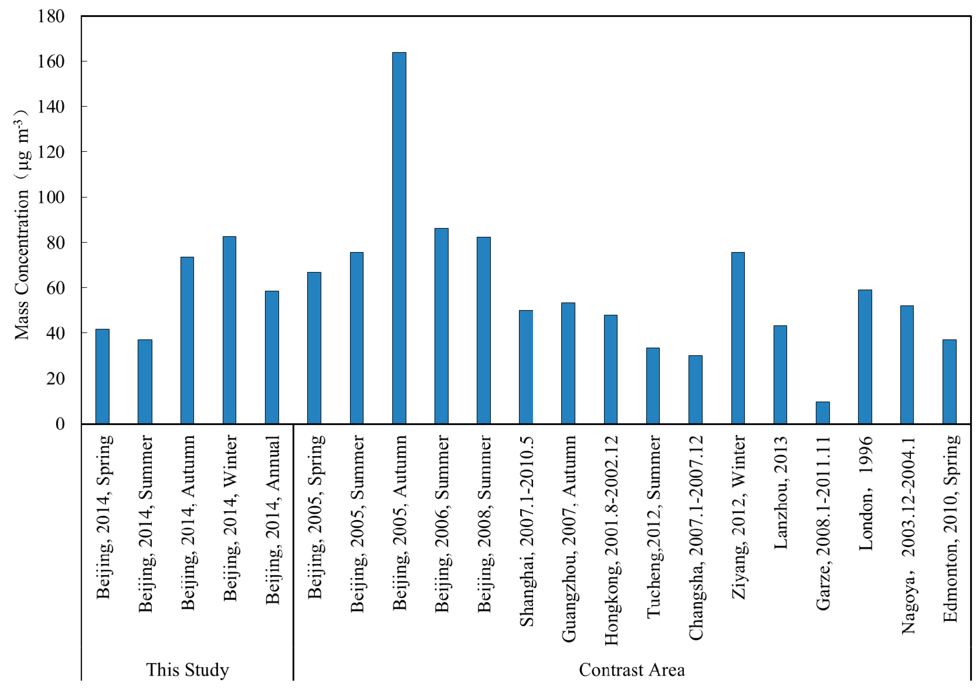
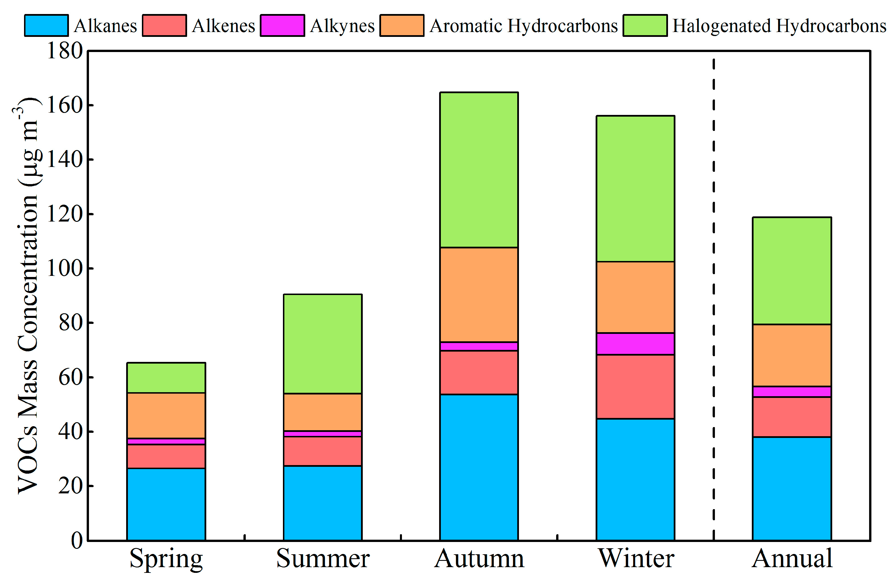
3.1. Concentration of VOCs and Inorganic Pollutants

The hourly mean mass concentration of 84 VOCs in the study area ranged from 9.11 to 567 μg·m⁻³, the daily mean mass concentration ranged from 24.1 to 324 μg·m⁻³, the annual mean mass concentration was 119 ± 109 μg·m⁻³ (Figure 2), and the mean mass concentration in spring, summer, autumn and winter was 65.0 ± 33.1, 90.9 ± 54.2, 164 ± 107 and 157 ± 102 μg·m⁻³, respectively, so the seasonal variation was such that spring < summer < winter < autumn. The annual mean mass concentration of halogenated hydrocarbons was the highest (39.1 ± 42.0 μg·m⁻³), followed by that of alkanes (38.1 ± 28.5 μg·m⁻³), aromatic hydrocarbons (22.9 ± 19.8 μg·m⁻³), alkenes (14.8 ± 14.9 μg·m⁻³), and alkynes (3.84 ± 3.51 μg·m⁻³) (Table 1). In spring, the mean mass concentration of alkanes was the highest, followed by aromatic hydrocarbons, halogenated hydrocarbons, alkenes and alkynes. In the other three seasons, the order was halogenated hydrocarbons, alkanes, aromatic hydrocarbons, alkenes, and alkynes (Figure 3). The mass concentration of the top ten VOCs accounted for 58.5% of the total 84 VOCs in spring, 61.1% in summer, 59.2% in autumn, and 60.8% in winter. The percentage of the top ten VOCs varied slightly with season. Propane, 1,1-dichloroethane, and m&p-xylene were in the top ten VOCs in all four seasons.

To better understand the VOCs pollution level in ambient air of typical urban areas in Beijing, the VOCs concentrations from our study were compared with those of other regions (Figure 4). Because of the large number of VOCs in past studies, 14 (ethane, propane, i-pentane, cyclopentane, me-cyclopentane, butane, ethylene, propene, isoprene, acetylene, benzene, toluene, ethylbenzene and m&p-xylenes) were selected for comparison. In our study, the annual mean concentration of 14 VOCs accounted for 44.8% of the total, and their pollution level reflected that of total VOCs to a certain extent. The sum of their concentrations for all the references included were 30%–80%, so we also think the 14 VOCs could represent some of the pollution characteristics of VOCs in the other cities. The mass concentration of 14 VOCs herein was lower than that of previous studies of Beijing. Concentrations in spring (41.6 μg·m⁻³), summer (37.2 μg·m⁻³) and autumn (73.5 μg·m⁻³) were lower than those in the same months of 2005 (66.9, 75.4 and 163 μg·m⁻³) [33], summer 2006 (86.2 μg·m⁻³) [34], and summer 2008 (82.3 μg·m⁻³) [35]. Beijing has gradually taken the air pollution control policy since 1982, but it did not include the VOCs control [36]. Since guide of advancing air pollution by joint prevention and control to improve regional air quality was publish by State Council 2010, it has become more attractive to control VOCs, which resulted in the highest concentration in 2005. Garzi 2008–2011 (9.7 μg·m⁻³) [37] was sited as a background, whose concentration will be lower than general sites. The mass concentration characteristics of 14 selected VOCs of four seasons showed a difference with the seasonal variation of 84 VOCs, but shared the common characteristic that spring and summer are lower than autumn and winter. Meanwhile, impacted by the emission sources and the photooxidation of single species of VOCs, there were seasonal differences. Compared with other regions (except for London in 1996, at 59.1 μg·m⁻³) [38], the mass concentrations of 14 VOCs in spring, summer, autumn and winter and annual mean mass concentrations were higher than those of Edmonton in spring 2010 (37.0 μg·m⁻³) [39], Tucheng in summer 2012 (33.5 μg·m⁻³) [40], Guangzhou in autumn 2007 (53.2 μg·m⁻³) [41], Ziyang in winter 2012 (75.6 μg·m⁻³) [42], Hong Kong in 2001 and 2002 (48.0 μg·m⁻³) [43], Changsha in 2007 (29.9 μg·m⁻³) [44], Lanzhou in 2013 (43.5 μg·m⁻³) [45], and Nagoya in 2003 and 2004 (52.0 μg·m⁻³) [46]. From these results, it is seen that current VOCs control measures have certain effects, but VOCs concentrations in ambient air are still higher in Beijing than in other regions. The VOCs pollution is still serious and it is necessary to take effective control measures to reduce VOCs in ambient air.

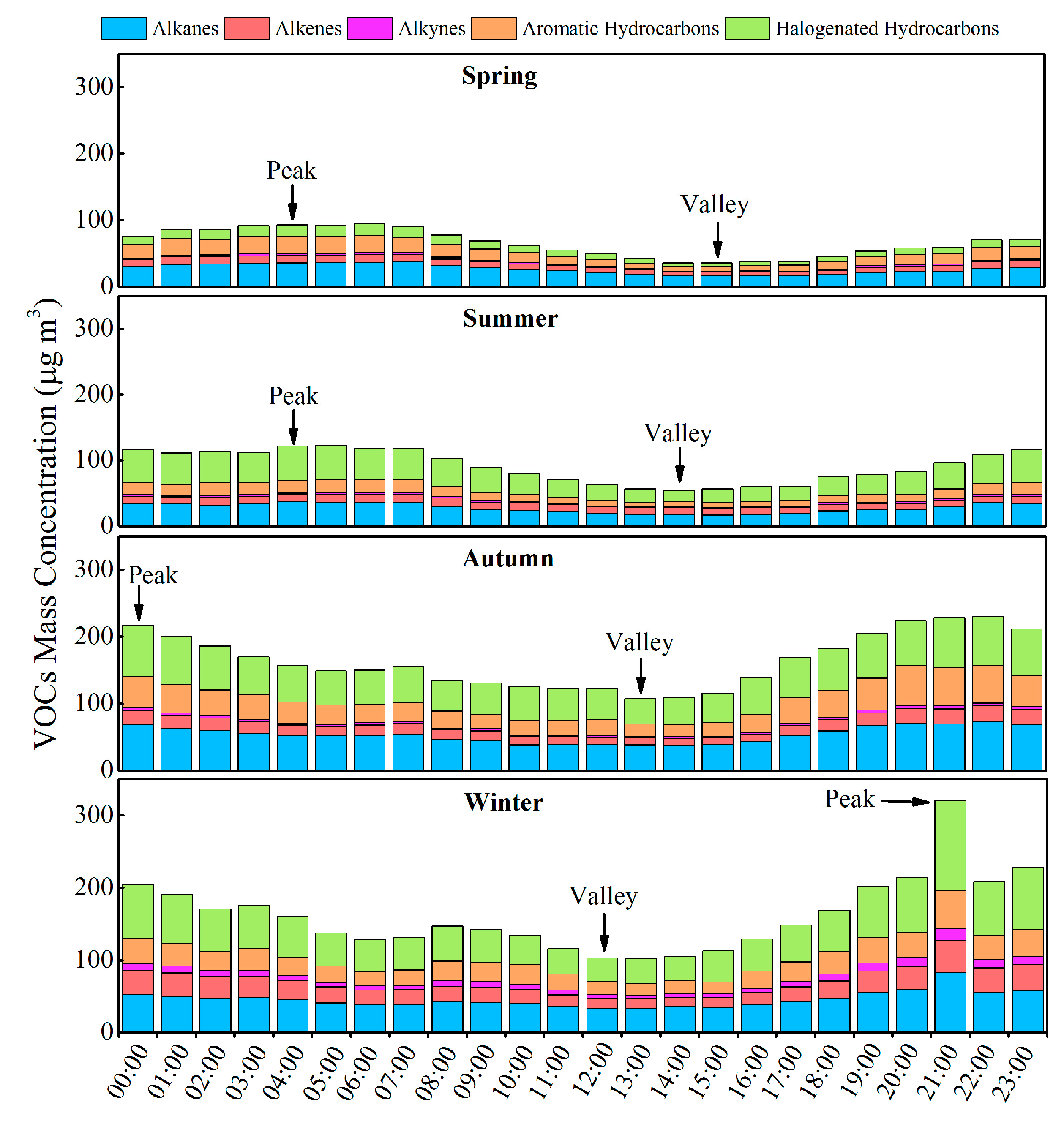
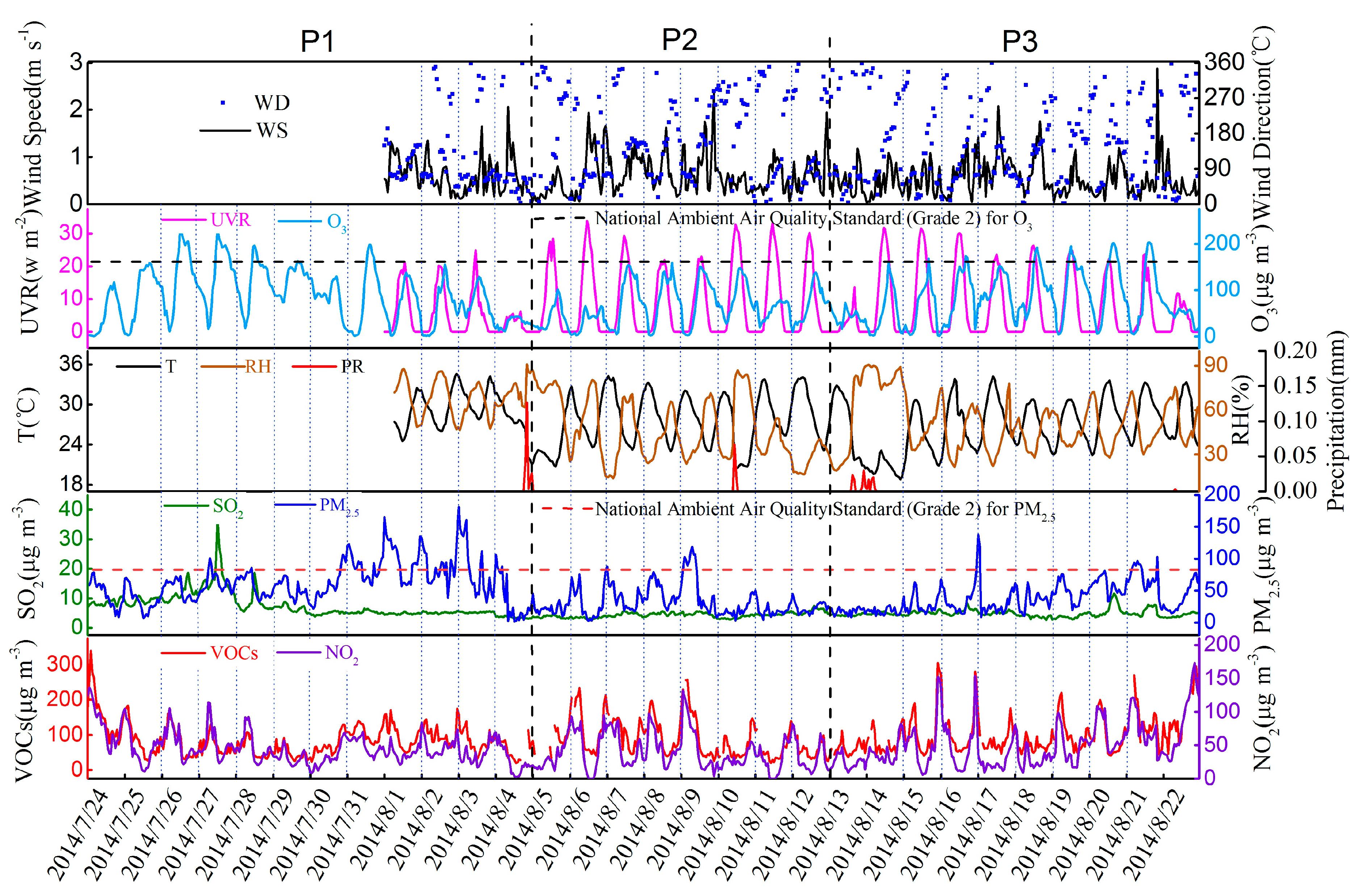
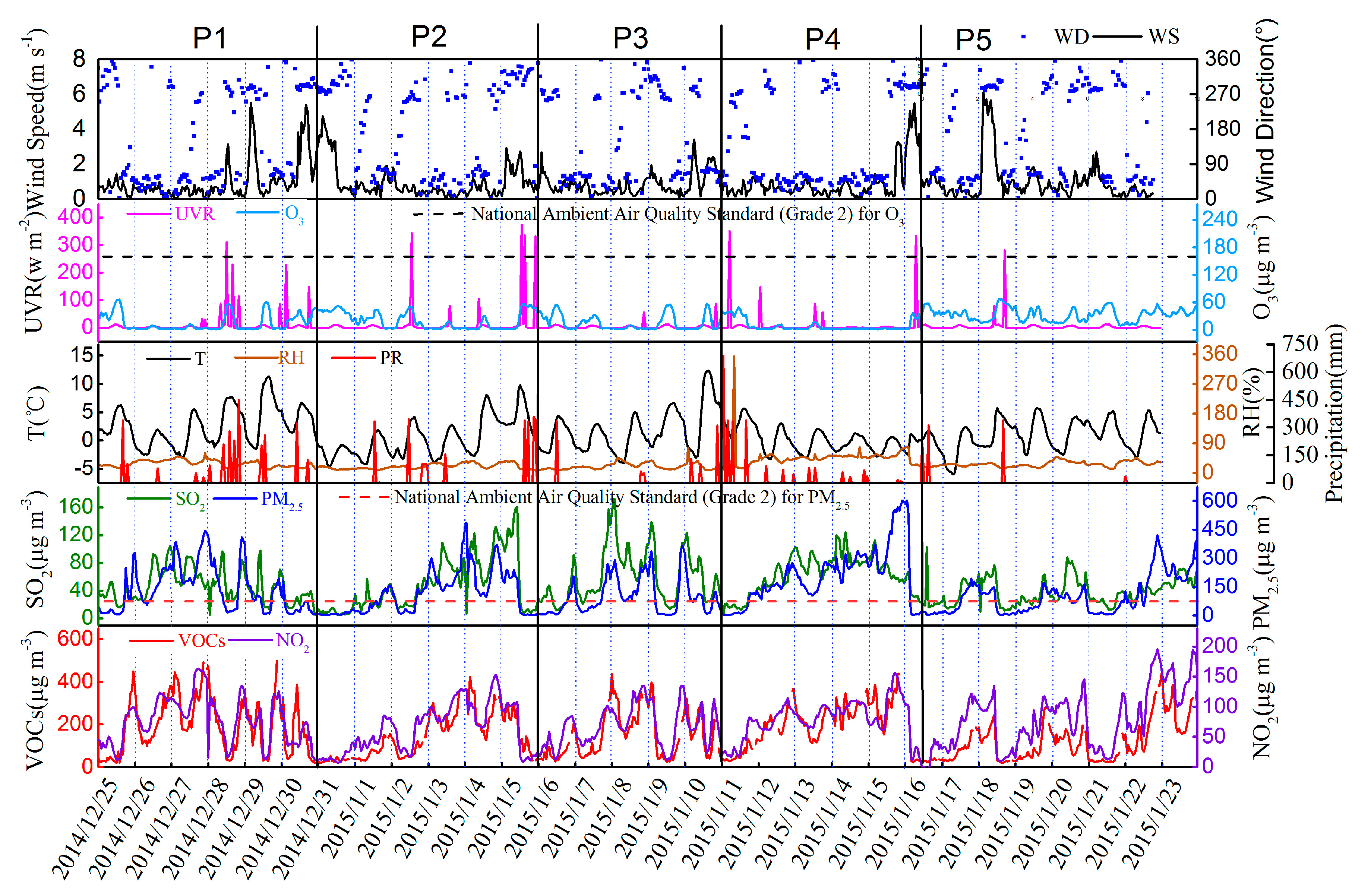
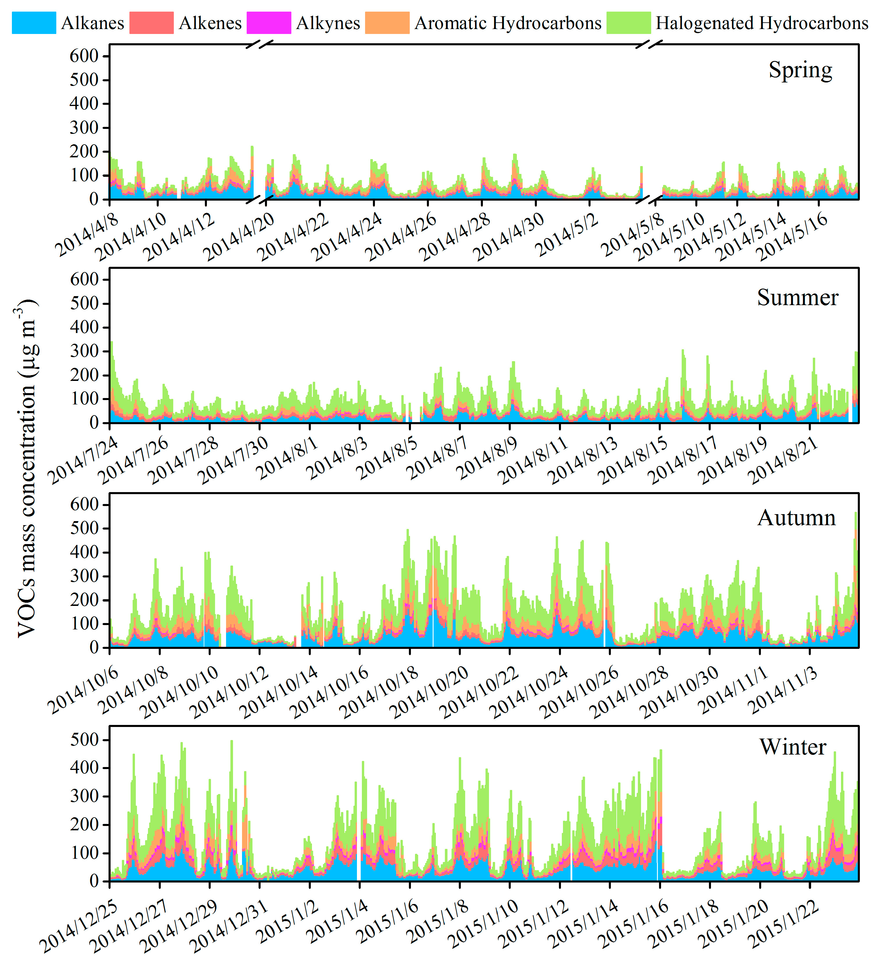
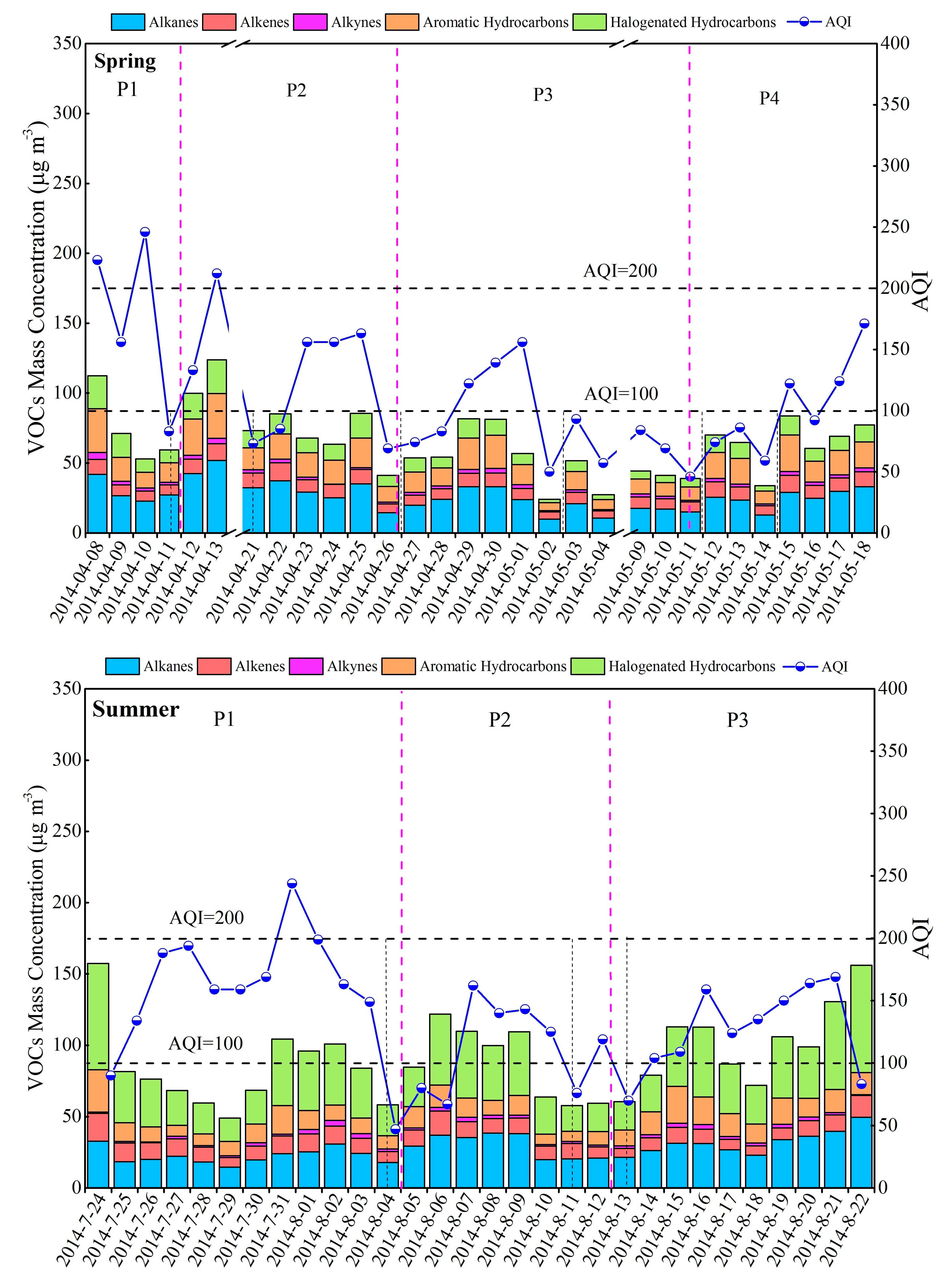
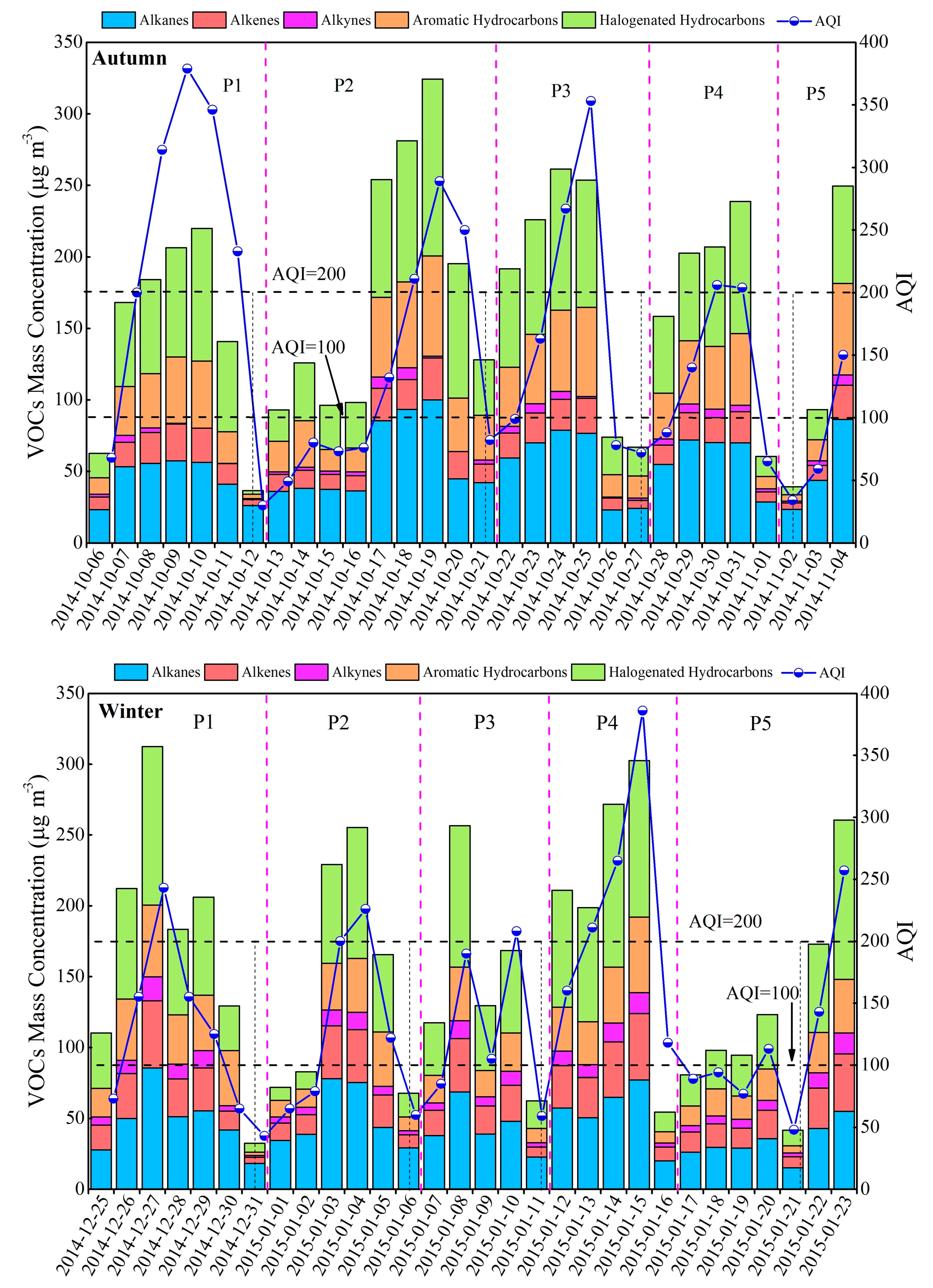
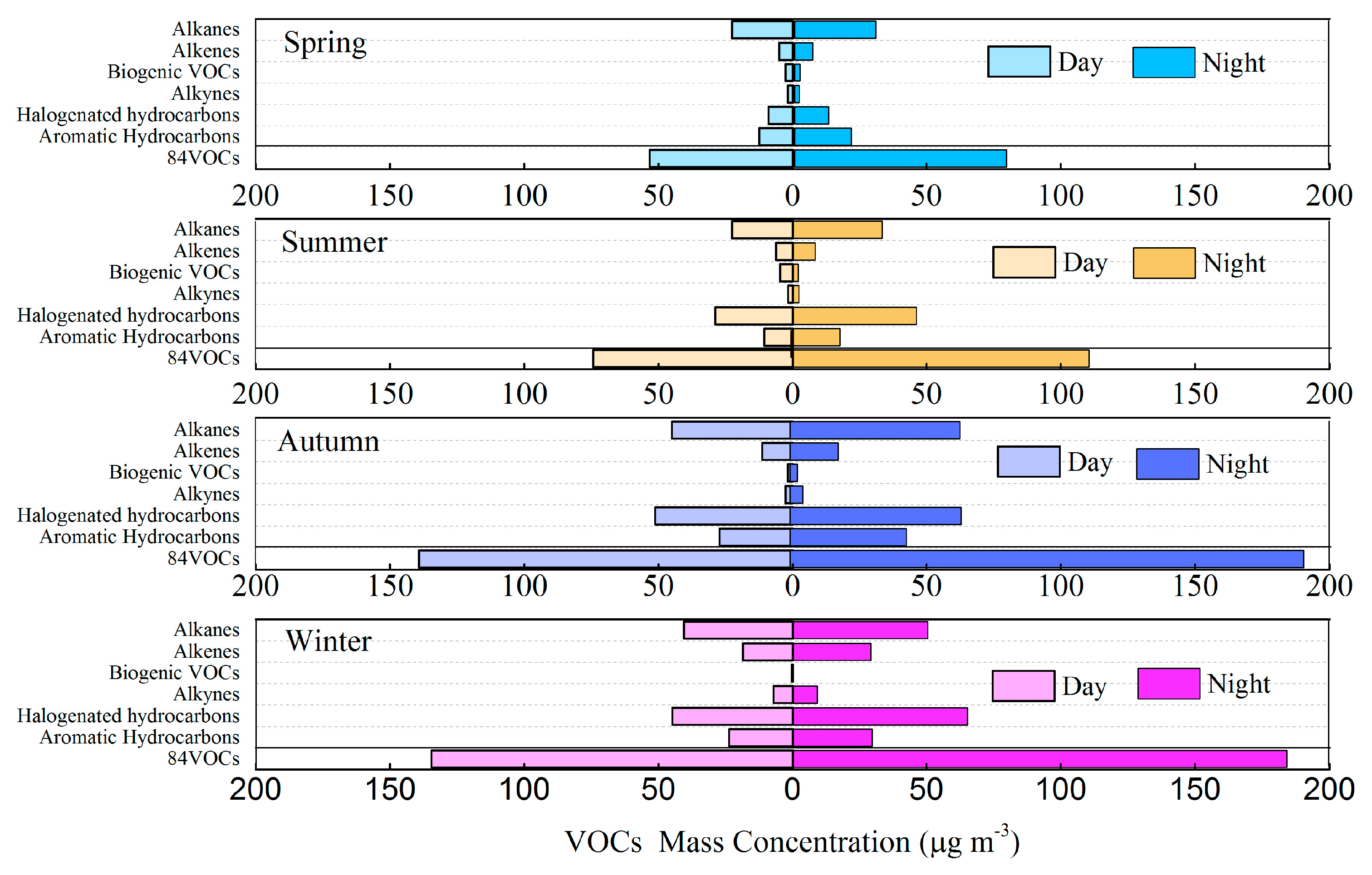
3.2. Variation Characteristics and Influential Factors

The mass concentration of 84 VOCs varied periodically in the study area. There were 8, 4, 5 and 6 variation periods in spring, summer, autumn and winter (Figure 5), respectively, with durations 2–3, 4–5, 4–5 and 3–4 days (the variation period was divided based on the air quality index (AQI) changed from the lowest point to another lowest point). According to the air pollutant concentration standard limits in Air Quality Standard GB 3095-2012 and ambient air quality index (AQI) in Ambient Air Quality Technical Requirements (Trial) (HJ 633-2012), the monitoring period was divided into three ozone pollution (O₃ > 160 μg·m⁻³) periods (P1, P2 and P3) in summer, and into five PM_2.5 pollution (PM_2.5 > 75 μg·m⁻³) periods (P1, P2, P3, P4 and P5) in Winter (the pollution event was divided based on the AQI changed from good to hazardous and to good again). The number of heavy pollution days in (AQI > 200) in spring, summer, autumn and winter were 3, 1, 12 and 8, respectively. The number of heavy pollution days in autumn and winter were greater than in spring and summer. The concentration variation of 84 VOCs was consistent with that of AQI, indicating that VOCs had a strong influence on ambient air quality in the study area.

Concentrations of 84 VOCs were higher at night than during daytime, except that the concentration of alkenes was higher in the daytime than at night during summer (Figure 6). The difference of mass concentration of those VOCs between night and day during spring, summer, autumn and winter was 26.5, 36.3, 51.2 and 49.7 μg·m⁻³, respectively, and diurnal variation of the mass concentration was strongest in autumn. One important reason for this is that solar radiation is stronger in the daytime, and a large amount of VOCs in ambient air were consumed in photochemical reactions. Another important reason is that the mixing of the surface air will also lead to this phenomenon, so the mass concentration of VOCs was lower during daytime. A third reason may be an increase of VOCs emission at night. According to traffic control measures of the Beijing Traffic Authority, large diesel vehicles were only allowed to enter the city via the Jingchang Expressway at night [47]. Moreover, the VOCs emission factor of diesel vehicles was several times larger than that of gasoline vehicles [48]. Therefore, VOCs accumulated at night. In summer, vegetation emitted substantial alkenes, resulting in a higher mass concentration of alkenes in the daytime. The reason why the difference of mass concentration of those VOCs between night and day in autumn is much higher than others needs to be further studied.

The diurnal concentration of halogenated hydrocarbons, alkanes, aromatic hydrocarbons, alkenes and alkynes varied with a V-shape in all four seasons (Figure 7), and the concentration of 84 VOCs was lowest during 12:00–5:00. The time of daily minimum values of halogenated hydrocarbons, alkanes, aromatic hydrocarbons, alkenes and alkynes gradually moved forward across the four seasons, i.e., minima occurred at 15:00 in spring, 14:00 in summer, 13:00 in autumn, and about 12:00 in winter. Maxima occurred at 4:00 in spring and autumn, 0:00 in autumn, and 21:00 in winter. Such variation may be related to change of VOCs sources, seasonal variation of solar radiation, and photochemical reactions in ambient air.

In summer, the trend of 84 VOCs in ambient air was consistent with those of conventional pollutants NO₂ and PM_2.5, opposite that of O₃, and dissimilar to that of SO₂ (Figure 8). Those VOCs had remarkable linear correlation with NO₂, significant correlation with PM_2.5 and O₃, and no correlation with SO₂. The VOCs were positively correlated with NO₂ and PM_2.5 and negatively correlated with SO₂ and O₃ (

Table 2. Correlation between 84 VOCs, conventional pollutants, and meteorological factors in summer (Pearson correlation coefficient).

Factors	VOCs	NO2	SO2	PM2.5	O3	T	RH	UVR
NO2 (n = 720)	0.71
SO2 (n = 720)	−0.03	0.10
PM2.5 (n = 720)	0.46	0.46	0.14
O3 (n = 720)	−0.42	−0.42	0.42	−0.15
T (n = 720)	−0.01	−0.12	−0.56	−0.16	−0.10
RH (n = 720)	0.13	0.03	−0.54	0.04	−0.49	0.66
UVR (n = 720)	−0.22	−0.36	−0.20	−0.28	0.21	0.48	0.03
PR (n = 720)	−0.11	−0.13	−0.10	−0.08	−0.04	−0.18	0.19	−0.06

Note: 0.0–0.2 means no correlation; 0.2–0.4 means weak correlation; 0.4–0.6 means moderate correlation; and 0.6–1.0 means strong correlation.

). The VOCs showed a trend similar to relative humidity (RH) and an opposite trend with temperature (T) and ultraviolet radiation (UVR). The correlation showed that the 84 VOCs had weak linear correlations with temperature, precipitation (PR), RH and UVR; they were positively correlated with RH and negatively correlated with T, PR and UVR. This analysis shows that high T and strong UVR in summer promote photochemical reactions in the atmosphere, increasing O₃ concentration, resulting in a relatively low mass concentration of VOCs in ambient air.

In winter, the trend of 84 VOCs in ambient air was consistent with that of the conventional gaseous pollutants NO₂, PM_2.5 and SO₂, and opposite that of O₃ (Figure 9). Those VOCs had remarkable linear correlation with NO₂ and PM_2.5, and significant correlation with SO₂ and O₃ (

Table 3. Correlation between 84 VOCs, conventional pollutants, and meteorological factors in winter (Pearson correlation coefficient).

Factors	VOCs	NO2	SO2	PM2.5	O3	T	RH	UVR
NO2 (n = 720)	0.79
SO2 (n = 720)	0.66	0.56
PM2.5 (n = 720)	0.89	0.80	0.60
O3 (n = 720)	−0.63	−0.57	−0.61	−0.56
T (n = 720)	−0.12	−0.01	−0.12	−0.18	0.33
RH (n = 720)	0.41	0.35	0.34	0.48	−0.42	−0.33
UVR (n = 720)	−0.12	−0.15	−0.11	−0.13	0.17	0.16	−0.09
PR (n = 720)	−0.10	−0.16	−0.12	−0.13	0.14	0.16	−0.11	0.13

Note: 0.0–0.2 means no correlation; 0.2–0.4 means weak correlation; 0.4–0.6 means moderate correlation; 0.6–1.0 means strong correlation.

). The VOCs were positively correlated with NO₂, SO₂ and PM_2.5, and negatively correlated with O₃. The VOCs showed a trend similar to RH and an opposite trend with T and UVR. The VOCs had weak linear correlation with T, PR, RH and UVR; they were positively correlated with RH and negatively correlated with T, PR and UVR. This analysis indicates that low T and weak UVR in winter weaken atmospheric photochemical reactions. Further, the atmospheric boundary layer is shallow in winter, which is not conducive to the diffusion of pollutants and favors the accumulation of VOCs.

High T, strong UVR, low PR, low RH, and strong atmospheric photochemical reactions in summer produced low VOCs concentrations in ambient air. In contrast, low T, weak UVR, abundant PR, and high RH in winter were not conducive to those reactions, so the concentration of VOCs was high. This analysis shows that photochemical reactions are strong under high T, low PR, low RH, and strong UVR, which can reduce the concentration of VOCs in ambient air.

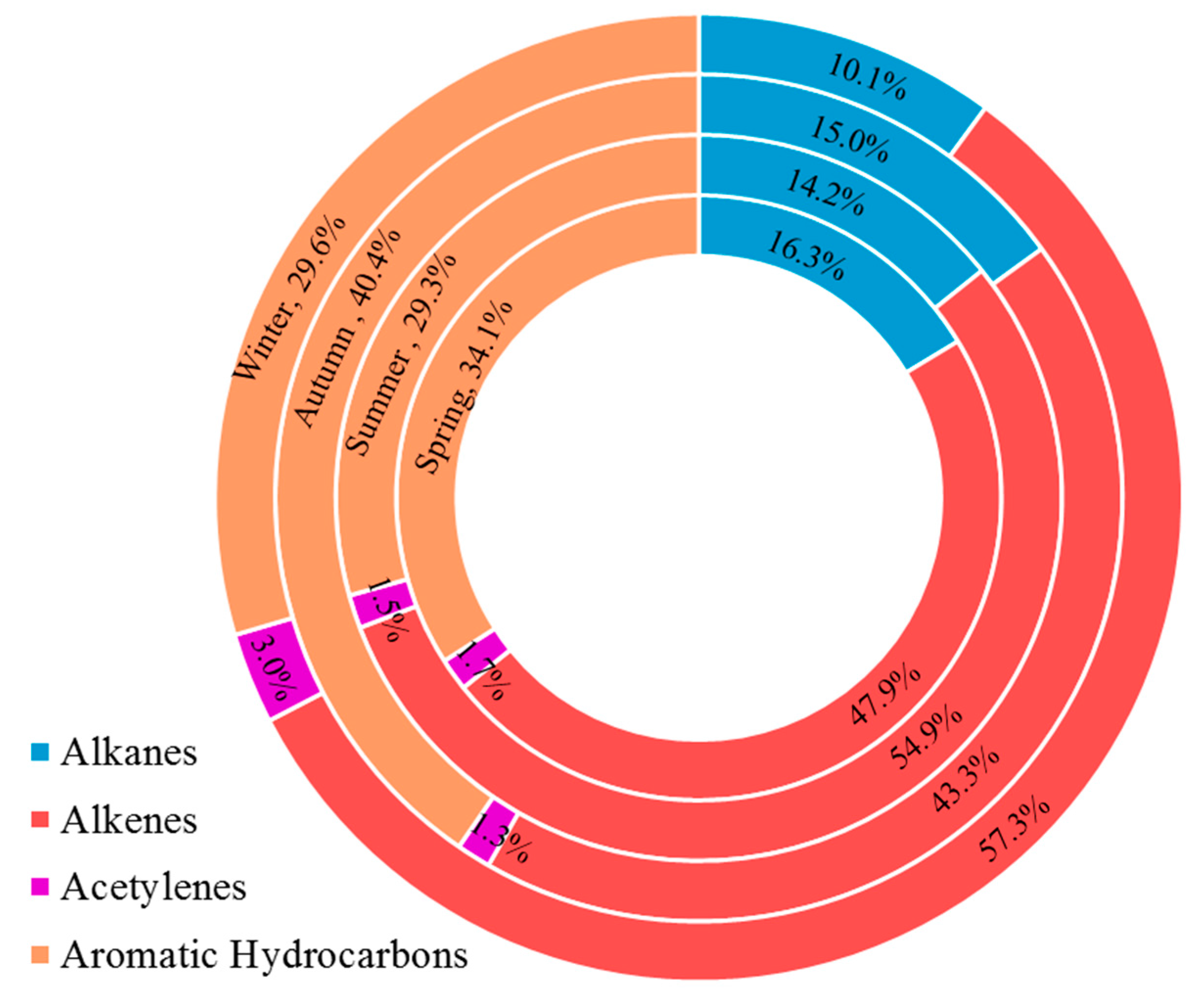
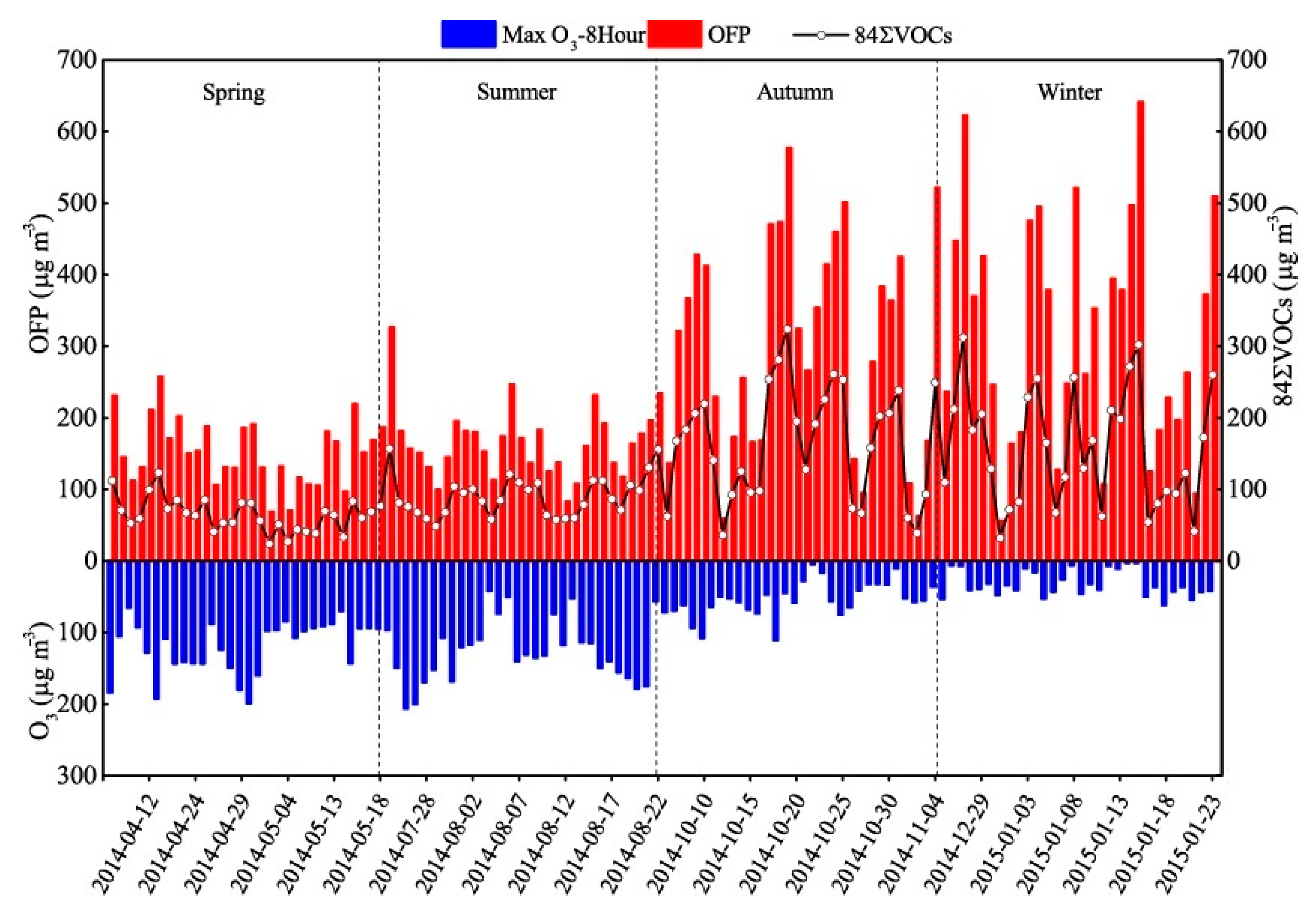
3.3. Ozone Formation Potential

Total contributions of 51 VOCs to OFP increased by season, with values in spring, summer, autumn and winter at 157 ± 96 μg·m⁻³ (the proportions of alkanes, alkenes, acetylenes and aromatic hydrocarbons were 16.3%, 47.9%, 1.7% and 34.1%, respectively), 169 ± 92 μg·m⁻³ (the proportions of alkanes, alkenes, acetylenes and aromatic hydrocarbons were 14.2%, 54.9%, 1.5% and 29.3%, respectively), 308 ± 235 μg·m⁻³ (the proportions of alkanes, alkenes, acetylenes and aromatic hydrocarbons were 15.0%, 43.3%, 1.3% and 40.4%, respectively) and 329 ± 242 μg·m⁻³ (the proportions of alkanes, alkenes, acetylenes and aromatic hydrocarbons were 10.1%, 57.3%, 3.0% and 29.6%, respectively), respectively (Figure 10). This seasonal variation was consistent with that of VOCs concentration. The greatest contribution to OFP was alkenes (122 ± 99 μg·m⁻³, accounting for 50.8%), followed by aromatic hydrocarbons (81.0 ± 87.5 μg·m⁻³, 33.7%), alkanes (32.2 ± 24.5 μg·m⁻³, 13.4%) and alkynes (4.79 ± 5.57 μg·m⁻³, 2.0%).

The top ten VOCs species were totally different among four seasons, which were ranked by the contributions to OFP. In spring, mass concentration of the top ten VOCs was 26.6 μg·m⁻³, accounting for 52.1% of the mean mass concentration of the 51 VOCs. Their OFP was 124 μg·m⁻³, accounting for 80.5% of total OFP of those VOCs. In summer, mass concentration of the top ten VOCs was 20.6 μg·m⁻³, accounting for 40.6% of total mean mass concentration. Their OFP was 133 μg·m⁻³, constituting 79.9% of the total OFP. In autumn, mass concentration of the top ten VOCs was 44.0 μg·m⁻³, representing 43.2% of the total mean mass concentration. Their OFP was 239 μg·m⁻³, or 78.6% of the total OFP. In winter, mass concentration of the top ten VOCs was 55.4 μg·m⁻³, accounting for 59.56% of the total mean mass concentration. Their OFP was 274 μg·m⁻³, or 86.0% of the total OFP. This analysis shows that to control ozone concentration in ambient air, it is necessary to control not only the total amount of VOCs but also species with high OFP in the air.

The daily OFP of 51 VOCs and mass concentration of 84 VOCs had similar trends (Pearson correlation coefficient was 0.981) (Figure 11); the daily maximum 8-h average ozone concentration had certain correlation with the OFP of 51 VOCs and concentration of 84 VOCs separately. The Pearson correlation coefficient of ozone and OFP, ozone and 84 VOCs, and OFP and 84 VOCs was 0.414, 0.383, and 0.984 (n = 120) respectively. This strong correlation between the OFP of 51 VOCs and VOCs shows that VOCs in ambient air have a major contribution to the formation of ozone in the study area. The OFP of 51 VOCs was greater than the daily maximum 8-h average ozone concentration on 25 days in spring, 20 days in summer, and all days in autumn and winter. This shows that the OFP of 51 VOCs was generally higher than the daily maximum 8-h average ozone concentration. However, oxygen-containing VOCs in ambient air, which have substantial OFP, were not measured. Moreover, the OFP of some observed VOCs was not examined, because their related factors were unavailable. Thus, the total OFP was underestimated. On some days in spring and summer, the OFP of 51 VOCs was less than the daily maximum 8-h average ozone concentration. The reason was that high T, strong UVR, low P and low RH in spring and summer produced strong photochemical reactions in ambient air. Thus, substantial VOCs were consumed, and the concentration of ozone increased. These conditions were opposite in autumn and winter. The low T, weak UVR, abundant P and high RH weakened the photochemical reactions, VOCs accumulated, and the concentration of ozone was relatively low. Thus, the OFP of 51 VOCs was generally higher than the daily maximum 8-hour average ozone concentration.

Different VOCs species have different photochemical reactivity and the photochemical age can be judged by their ratios [18,22,49,50]. Different types of VOCs in ambient air have varying chemical activities, and photochemical age of an air mass can be estimated using the ratio of VOCs. Acetylene is more photochemical-active than ethane, and m&p-xylenes is more photochemical-active than ethylbenzene. In the atmosphere, the four substances above are continuously consumed at different reaction rates. The ratios of ethane/acetylene and ethylbenzene/m&p-xylenes vary during photochemical reaction. The larger the two ratios, the greater the photochemical age of the air mass and the longer its transport time to the monitoring site. For a fresh air mass, ethane/acetylene and ethylbenzene/m&p-xylenes ratios were about 0.47 [51] and 0.42 [52,53]. In the four seasons, observed ethane/acetylene ratios were 2.04 ± 1.07, 1.49 ± 5.02, 2.3 ± 11.2 and 1.31 ± 0.53, and ethylbenzene/m&p-xylenes ratios were 0.65 ± 1.20, 0.57 ± 0.17, 0.53 ± 0.13 and 0.40 ± 0.18, respectively. Ethane/acetylene was > 1.0 and ethylbenzene/m&p-xylenes ~0.5, and the ratios were smallest in winter, indicating that air masses in the study area had a certain degree of aging. This degree was strong in spring and autumn and low in winter. This indicated that the ambient air was mainly impacted by fresh emission sources in winter and by distant sources in spring, summer and autumn.

3.4. Secondary Organic Aerosol Formation Potential

The SOAFP of 30 VOCs varied with season. It was greatest in autumn (2.36 ± 1.83 μg·m⁻³) (the proportions of alkanes, alkenes and aromatic hydrocarbons were 16.4%, 1.62% and 82.0%, respectively), followed by winter (1.60 ± 1.10 μg·m⁻³) (the proportions of alkanes, alkenes and aromatic hydrocarbons were 16.0%, 0.97% and 83.1%, respectively), spring (1.05 ± 0.80 μg·m⁻³) (the proportions of alkanes, alkenes and aromatic hydrocarbons were 9.54%, 2.34% and 88.1%, respectively), and summer (0.91 ± 0.64 μg·m⁻³) (the proportions of alkanes, alkenes and aromatic hydrocarbons were 21.2%, 4.27% and 74.6%, respectively) (Figure 12). This reveals a trend of higher potential in autumn and winter and lower in spring and summer. The greatest contribution to SOAFP was aromatic hydrocarbons (1.22 ± 1.23 μg·m⁻³, accounting for 82.3%), followed by alkanes (0.23 ± 0.21 μg·m⁻³, 15.8%) and alkenes (0.03 ± 0.05 μg·m⁻³, 1.98%).

Toluene, dodecane, m&p-xylenes, ethylbenzene, 1,3,5-TMB and benzene were in the top ten VOCs of SOAFP contribution in all four seasons. In spring, mass concentration of the top ten VOCs was 18.3 μg·m⁻³, accounting for 90.6% of mean mass concentration of the 30 VOCs. Their SOAFP was 1.00 μg·m⁻³, making up 95.5% of the total SOAFP of those VOCs. In summer, mass concentration of the top ten VOCs was 16.2 μg·m⁻³, constituting 86.8% of mean mass concentration of the 30 VOCs. Their OFP was 0.85 μg·m⁻³, or 93.8% of the total SOAFP. In autumn, mass concentration of the top ten VOCs was 41.3 μg·m⁻³, accounting for 88.5% of mean mass concentration of the 30 VOCs. Their SOAFP was 2.25 μg·m⁻³, or 95.1% of the total SOAFP. In winter, mass concentration of the top ten VOCs was 31.1 μg·m⁻³, representing 90.9% of mean mass concentration of the 30 VOCs. Their SOAFP was 1.53 μg·m⁻³, or 95.6% of the total SOAFP. The above analysis shows that to control the concentration of particulate matter in the ambient air, it is necessary to control not only the total amount of VOCs but also species with greater SOAFP in ambient air.

The mass concentration of SOAs, SOAFP of 30 VOCs, and mass concentration of 84 VOCs had similar variations (Figure 13). Their correlations were significant. The correlation coefficients of SOAs with SOAFP, SOAs with 84 VOCs, and SOAFP with 84 VOCs, were 0.650, 0.875, and 0.894, respectively. Such strong correlation shows that VOCs in ambient air have a major contribution to the formation of SOAs in the study area.

The mass concentration of SOAs was higher than the SOAFP during the study. The main reason was that the 84 VOCs observed did not include all species with SOAFP. The SOAFP of some VOCs were not calculated because their related factors were unavailable. Further, the FAC model was based on smog chamber experiments, which were affected by factors such as T, UVR, RH, acidity of particulate matter, and concentration of precursors. Thus, that model underestimated the SOAFP [52].

3.5. Health Risk Assessment

The non-carcinogenic HQ of 22 toxic and harmful VOCs in spring, summer, autumn and winter was 0–4.85 × 10⁻⁰², 0–9.70 × 10⁻⁰², 0–2.13 × 10⁻⁰¹ and 0–2.05 × 10⁻⁰¹, respectively. HI (sum of HQ) in the four seasons was 9.96 × 10⁻⁰², 1.41 × 10⁻⁰¹, 3.20 × 10⁻⁰¹ and 3.78 × 10⁻⁰¹, respectively (

Table 4. Non-carcinogenic risk assessment result of 22 VOCs.

Species	RfC (mg·m−3)	HQ
		Spring	Summer	Autumn	Winter
benzene	3.00 × 10−02	1.26 × 10−02	1.12 × 10−02	2.43 × 10−02	3.58 × 10−02
1,3-butadiene	2.00 × 10−03	2.22 × 10−02	1.75 × 10−02	4.42 × 10−02	8.14 × 10−03
vinylchloride	1.00 × 10−01	0.00 × 10+00	0.00 × 10+00	0.00 × 10+00	5.39 × 10−03
dichloromethane	6.00 × 10−01	8.13 × 10−07	0.00 × 10+00	0.00 × 10+00	5.38 × 10−05
tetrachloroethene	4.00 × 10−02	4.68 × 10−03	2.18 × 10−03	2.62 × 10−03	1.84 × 10−02
CCl4	1.00 × 10−01	8.23 × 10−07	2.16 × 10−06	0.00 × 10+00	0.00 × 10+00
1,2-dibromoethane	9.00 × 10−03	3.67 × 10−04	4.63 × 10−04	8.86 × 10−05	4.92 × 10−05
1,3-dicl-propen	2.00 × 10−02	3.24 × 10−03	5.81 × 10−03	1.55 × 10−02	1.33 × 10−02
trichloroethene	2.00 × 10−03	4.85 × 10−02	9.70 × 10−02	2.13 × 10−01	2.05 × 10−01
1,2-dicl-propane	4.00 × 10−03	9.73 × 10−04	0.00 × 10+00	0.00 × 10+00	7.78 × 10−02
ethylbenzene	1.00 × 10+00	2.58 × 10−04	2.81 × 10−04	6.97 × 10−04	4.19 × 10−04
styrene	1.00 × 10+00	5.54 × 10−05	1.96 × 10−04	1.27 × 10−04	6.49 × 10−05
cyclohexane	6.00 × 10+00	4.73 × 10−06	4.95 × 10−06	1.28 × 10−05	5.15 × 10−06
i-propylbenzene	4.00 × 10−01	1.90 × 10−06	1.26 × 10−05	2.50 × 10−05	1.50 × 10−05
1,4-dicl-benzene	8.00 × 10−01	6.67 × 10−05	8.67 × 10−05	1.99 × 10−04	5.91 × 10−05
n-hexane	7.00 × 10−01	2.93 × 10−04	2.27 × 10−04	5.57 × 10−04	3.36 × 10−04
chloromethane	9.00 × 10−02	0.00 × 10+00	0.00 × 10+00	0.00 × 10+00	5.85 × 10−04
naphtalene	3.00 × 10−03	0.00 × 10+00	0.00 × 10+00	0.00 × 10+00	0.00 × 10+00
1,1,1-tricl-ethane	5.00 × 10+00	1.33 × 10−08	0.00 × 10+00	3.77 × 10−07	2.42 × 10−07
toluene	5.00 × 10+00	2.23 × 10−04	9.46 × 10−05	2.87 × 10−04	1.48 × 10−04
m&p-xylenes	1.00 × 10−01	1.55 × 10−03	2.19 × 10−04	4.58 × 10−03	1.32 × 10−03
o-xylene	1.00 × 10−01	4.52 × 10−03	5.47 × 10−03	1.38 × 10−02	1.04 × 10−02
HI		9.96 × 10−02	1.41 × 10−01	3.20 × 10−01	3.78 × 10−01

). The carcinogenic risk of benzene in the four seasons, 1,3-butadiene in spring, summer and autumn, vinylchloride in winter, 1,2-dibromoethane in spring and summer, and 1,3-dicl-propen and trichloroethene in autumn and winter, exceeded 1.00 × 10⁻⁰⁶ (

Table 5. Carcinogenic risk assessment result of nine VOCs.

Species	IUR (m3·µg−1)	Risk
		Spring	Summer	Autumn	Winter
benzene	7.80 × 10−06	2.94 × 10−06	2.61 × 10−06	5.68 × 10−06	8.37 × 10−06
1,3-butadiene	3.00 × 10−05	1.33 × 10−06	1.05 × 10−06	2.65 × 10−06	4.89 × 10−07
vinylchloride	8.80 × 10−06	0.00 × 10+00	0.00 × 10+00	0.00 × 10+00	4.74 × 10−06
dichloromethane	1.00 × 10−08	4.88 × 10−12	0.00 × 10+00	0.00 × 10+00	3.23 × 10−10
tetrachloroethene	2.60 × 10−07	4.87 × 10−08	2.27 × 10−08	2.72 × 10−08	1.92 × 10−07
CCl4	6.00 × 10−06	4.94 × 10−10	1.30 × 10−09	0.00 × 10+00	0.00 × 10+00
1,2-dibromoethane	6.00 × 10−04	1.98 × 10−06	2.50 × 10−06	4.78 × 10−07	2.66 × 10−07
1,3-dicl-propen	4.00 × 10−06	2.59 × 10−07	4.65 × 10−07	1.24 × 10−06	1.06 × 10−06
trichloroethene	4.10 × 10−06	3.98 × 10−07	7.95 × 10−07	1.74 × 10−06	1.68 × 10−06

). The US EPA has stated that pollutants do not have significant non-carcinogenic effects on human health for HQ < 1; the acceptable carcinogenic risk for adults is 1 × 10⁻⁰⁶. HI of the observed 22 toxic and harmful VOCs in our study was <1, so they had no non-carcinogenic risk. However, the carcinogenic risk of benzene over the entire study and 1,3-butadiene, vinylchloride, 1,2-dibromoethane, 1,3-dicl-propen and trichloroethene in certain periods exceeded 1 × 10⁻⁰⁶, so they had a clear impact on human health and carcinogenic risk. Considering the impact on human health and the influence on environment of these species, vinylchloride, 1,2-dibromoethane, 1,3-dicl-propen and trichloroethene were the riskiest species which should be paid more attention [54]. Long-term exposure could harm human health. According to the exposure parameters of the Chinese population, Chinese population spend most of their day time indoors (1213 min·day⁻¹), and the concentrations of certain poisonous and harmful VOCs are higher indoors. Therefore, it was more important to study health risk of poisonous and harmful VOCs indoors, and the research should draw high attention [29].

Benzene series are a group of toxic and harmful VOCs in ambient air. Long-term exposure to this series stimulates human skin and mucous membrane, and produces chronic or acute injury to human respiratory, hematopoietic and nervous systems [55]. Of the 17 benzene series studied, BTEX (benzene, toluene, ethylbenzene, m&p-xylenes), o-xylene and styrene are among the toxic and harmful air pollutants published by the US EPA. Therefore, data of these six substances in Beijing were compared with data of Beijing and other cities from other studies. The results show that the HQ of BTEX and styrene in ambient air was in the range 5.56 × 10⁻⁰⁵ to 2.28 × 10⁻⁰¹, the HI of BTEX and styrene was <1, and their non-carcinogenic risk was within the safe range. The HQ of benzene was larger than that of other benzene series, indicating that benzene was the major non-carcinogenic risk to human health in benzene series of the ambient air. The carcinogenic risk of benzene in ambient air was >1 × 10⁻⁰⁶ in all cities, showing a potential carcinogenic risk. The results of our study again show that it is very necessary to take strict measures to control benzene pollution in ambient air of China, and environmental and concentration standards for benzene should be developed as early as possible [17,28]. Compared with previous studies of Beijing, the carcinogenic risk of benzene in our study was the smallest (4.90 × 10⁻⁰⁶) (

Table 6. Health risk assessment results of benzene series in ambient air, in present study and of other cities in China.

City	Benzene		Toluene	Ethylbenzene	m&p-Xylenes	O-Xylene	Styrene		Reference
	Carcinogenic Risk	HQ	HQ	HQ	HQ	HQ	HQ	HI
Beijing (2014–2015)	4.90 × 10−06	2.09 × 10−02	1.88 × 10−04	4.13 × 10−04	1.92 × 10−03	8.55 × 10−03	1.11 × 10−04	3.21 × 10−02	This work
Beijing (2013)	8.80 × 10−06	3.76 × 10−02	5.84 × 10−04	1.15 × 10−03	1.53 × 10−02	7.19 × 10−03	8.70 × 10−05	6.19 × 10−02	[17]
Beijing (2008–2010)	1.34 × 10−05	5.73 × 10−02	1.08 × 10−03	1.19 × 10−03	2.09 × 10−02	5.32 × 10−03	1.60 × 10−04	8.60 × 10−02	[56]
Beijing (2012)	4.19 × 10−05	1.57 × 10−01	2.39 × 10−02	3.29 × 10−03	8.06 × 10−03	3.53 × 10−03	-	1.96 × 10−01	[28]
Beijing (2011)	2.21 × 10−05	1.58 × 10−01	-	1.69 × 10−02	7.76 × 10−03 *		1.06 × 10−02	1.93 × 10−01	[57]
Shanghai (2007–2010)	7.55 × 10−06	3.23 × 10−02	5.93 × 10−04	0.00 × 10+00	1.02 × 10−02	3.56 × 10−03	9.99 × 10−05	4.67 × 10−02	[58]
Lanzhou (2013)	8.09 × 10−06	3.46 × 10−02	1.27 × 10−04	4.07 × 10−04	6.18 × 10−03	2.76 × 10−03	1.28 × 10−04	4.42 × 10−02	[45]
Ganzi (2008–2011)	3.00 × 10−06	1.28 × 10−02	5.56 × 10−05	2.04 × 10−04	2.04 × 10−03	2.26 × 10−03	1.64 × 10−04	1.76 × 10−02	[37]
Guangzhou (2005)	9.97 × 10−06	4.26 × 10−02	8.85 × 10−04	8.44 × 10−04	1.06 × 10−02	5.17 × 10−03	1.57 × 10−04	6.03 × 10−02	[33]
Guangzhou (2009)	5.34 × 10−05	2.28 × 10−01	3.95 × 10−03	4.26 × 10−03	3.06 × 10−03	2.42 × 10−03	-	2.42 × 10−01	[59]
Tianjin (2008)	2.18 × 10−05	-	-	-	-	-	-	-	[60]
Hangzhou (2006–2007)	1.22 × 10−05	1.22 × 10−01	2.05 × 10−02	2.30 × 10−03	5.25 × 10−02		6.00 × 10−04	1.98 × 10−01	[61]

“-” means there are no related data in this paper, “*” refers to non-carcinogenic risk HI of xylenes.

), indicating that current pollution control measures in the city have had some effect, but there remains carcinogenic risk. More attention should be paid to this issue, and stringent control measures should be continuously implemented. It is noteworthy that human exposure parameters of the US EPA were used to evaluate the impact of VOCs in ambient air on human health in the referenced studies. This is likely to overestimate the human health risks of Chinese populations. To more accurately reflect the risks of toxic and harmful VOCs to human health, it is necessary to use exposure parameters of Chinese populations to assess the risks of toxic and harmful VOCs to human health in the country.

3.6. Source Apportionment

After several rounds of PMF calculation, adjusting relevant parameters, referring to relevant guides, and the resulted stable Q values, sources of VOCs in ambient air and their contributions were determined. There were five VOC sources in spring: vegetation emission, solvent usage, industrial process, vehicle exhaust, and fossil fuel combustion. There were four sources in the other three seasons: vegetation emission, solvent usage, industrial process, and vehicle exhaust in summer and autumn; and solvent usage, industrial process, vehicle exhaust and fossil fuel combustion in winter (Figure 14). In spring, the percentage of isoprene, a significant tracer for vegetation emission sources [62], was high. Because spring is the growth period of vegetation, and the studies made in Beijing area earlier showed that plants in Beijing could emit amount of benzene series and fallen leaves in Beijing could also emit amount of benzene series, we considered factor 1 in spring season as vegetation sources, although there were some proportions of benzene and toluene in factor 1 in the PMF analysis for spring season [63,64]. It was concluded that factor 1 was a vegetation emission source. For factor 2, the proportion of alkanes and alkenes was large. Alkanes and alkenes in ambient air were mainly from industrial and commercial activities during the observation period [43], so factor 2 was a solvent usage source. For factor 3, the proportions of benzene, toluene and xylene were large. BTEX and styrene were mainly from surrounding industrial process emissions [65], so we conclude that factor 3 was an industrial process source. For factor 4, trans-2-butene, cis-2-butene and propene accounted for a large proportion, and the main components of vehicle exhaust were trans-2-butene, cis-2-butene, benzene, toluene, propene and others [66,67,68]. i-Pentane, ethane and propane also constituted a large proportion, and the major components of volatile gas from vehicles were alkanes and monocyclic aromatic hydrocarbons. We conclude that factor 4 was a vehicle exhaust source. For factor 5, alkenes accounted for a large proportion, and it was initially identified as a fossil fuel combustion source [65]. Similarly, we determined that factor 1 was a vegetation emission source in summer and autumn, factor 2 was a solvent usage source, factor 3 an industrial process source, and factor 4 a vehicle exhaust source. In winter, factor 1 was a solvent usage source, factor 2 an industrial process source, factor 3 a vehicle exhaust source, and factor 4 a fossil fuel combustion source.

The contributions of emission sources from high to low were: vehicle exhaust, vegetation emission, solvent usage, industrial process, and fossil fuel combustion in spring; vehicle exhaust, solvent usage, industrial process, and vegetation emission in summer; vehicle exhaust, solvent usage, vegetation emission and industrial process in autumn; vehicle exhaust, fossil fuel combustion, solvent usage, and industrial process in winter (Figure 15). VOCs from vehicle exhausts accounted for the largest proportion (~40%) of total VOCs in the four seasons, and increased with the above seasonal order. This result is similar to that of Song et al. (43%) [69], indicating that the major source of VOCs is related to the use of vehicles. Owing to the impact of Temperature (T), substantial VOCs were emitted by vehicles in summer and autumn. T was low in winter but vehicle use increased because of cold weather, so VOCs from vehicle exhausts increased. VOCs from vegetation emission sources accounted for ~15% in spring, summer and autumn, and were greatest in spring. There was no emission from vegetation emission sources in winter. The main reason is that vegetation grows in spring and their emissions were higher; in summer, T and VOCs activity in ambient air were high. Thus, VOCs might have been consumed by photochemical reactions in the ambient air during transmission, and the contribution of vegetation emission sources was underestimated in summer. Fossil fuel combustion sources only contributed to VOCs in ambient air during spring and winter, with a larger proportion in winter than in spring. This variation was affected by heating. The proportion of fossil fuel combustion decreased with warming weather in spring. The industrial process source was stable across the seasons. This proportion was ~10% in spring, autumn and winter, and larger in summer. The reason may be that southerly winds prevailed in that season and there were many factories south of Beijing. The proportion of the solvent usage source was ~25% in summer and autumn, and ~15% in spring and ~17% in winter. Compared to spring and winter, T was higher and solvent volatility was greater in summer and autumn. Therefore, the solvent usage source proportion was greater in those two seasons. Because the vehicle exhaust source had an important contribution and automobiles had a large proportion within that source, there should be more stringent control of automobiles.

The ratio of benzene to toluene can also be used to determine the source of VOCs in ambient air during the study period. That ratio in spring, summer, autumn and winter was 0.34, 0.71, 0.51 and 1.45, respectively. The ratio is impacted by vehicle exhausts, use of paint, and solvent evaporation in spring, while it is mainly influenced by vehicle exhausts in summer and autumn, and by those emissions and coal and biomass combustion in winter. The ratio of benzene to toluene also shows that vehicle exhaust was the main source of VOCs in the study area, consistent with results of the PMF analysis above.

4. Conclusions

In this study, VOCs were measured continuously using an online VOCs monitoring instrument in a typical urban area of Beijing, from February 2014 through January 2015. Pollution characteristics, health risks, and source apportionment of VOCs in ambient air in typical urban areas of Beijing were studied. The annual average concentration of VOCs in ambient air was 119 μg·m⁻³, and the hourly mean concentration was 9.11–567 μg·m⁻³. VOCs pollution in the ambient air of Beijing has been alleviated in recent years, but it is still serious compared to other regions. In the study area, VOCs with the largest proportions were alkanes in spring and halogenated hydrocarbons in summer, autumn and winter. Concentration variation of 84 VOCs was consistent with that of the ambient air quality index, indicating that VOCs had a clear influence on ambient air quality in the study area. Affected by human and meteorological factors, VOCs concentrations were highest in autumn, followed by summer, winter and spring. Generally, concentrations were higher at night and lower in the daytime. The diurnal variation was V-shaped, with smallest values from 12:00 to 15:00. VOCs concentrations were relatively high under low T, weak UVR, abundant P and high RH. Impacted by the concentration and activity of VOCs, the largest contributions to OFP and SOAFP were from alkenes and aromatic hydrocarbons, respectively. The 22 toxic and harmful VOCs did not pose non-carcinogenic risk to the exposed population, but five toxic and harmful VOCs such as benzene had carcinogenic risk. These results were compared with those from other cities, revealing that benzene was a common carcinogenic risk in urban ambient air. Therefore, it is suggested that China establish health criteria and ambient air quality standards for benzene in ambient air as soon as possible, to reduce its carcinogenic risk in urban environments. The main sources of VOCs during the study were vehicle exhaust, solvent usage, and industrial process. To improve air quality in Beijing and reduce the risk of disease, it is necessary to strengthen control of VOCs from vehicle exhausts, solvent usage and industrial process, and reduce emissions of toxic and harmful VOCs.

References

1. Maroni, M.; Seifert, B.; Lindvall, T. Indoor Air Quality: A Comprehensive Reference Book; Elsevier Science: Amsterdam, The Netherlands, 1995. [Google Scholar]
2. World Health Organization (WHO). Air Quality Guidelines for Europe, 2nd ed.; WHO Regional Publications: Rome, Italy; World Health Organisation Regional Office for Europe: Copenhagen, Denmark, 1987. [Google Scholar]
3. Molhave, L.; Clausen, G.; Berglund, B.; Deaurriz, J.; Kettrup, A.; Lindvall, T.; Maroni, M.; Pickering, A.C.; Risse, U.; Rothweiler, H.; et al. Total Volatile Organic Compounds (TVOC) in Indoors Air Quality Investigations. Indoor Air J. 1997, 7, 225–240. [Google Scholar] [CrossRef]
4. Ministry of Environmental Protection of the People’s Republic of China. 2015 Report on the State of the Environment in China; Ministry of Environmental Protection of the People’s Republic of China: Beijing, China, 2016.
5. Beijing Municipal Environmental Protection Bureau. 2015 Report on the State of the Environment in Beijing; Beijing Municipal Environmental Protection Bureau: Beijing, China, 2015. Available online: http://www.bjepb.gov.cn/bjhrb/xxgk/ywdt/hjjc/qtjcgzdtxx/513514/index.html (accessed on 13 March 2016).
6. An, J.L. Ozone production efficiency in Beijing area with high NOx emissions. Acta Sci. Cirunmstantiae 2006, 26, 652–657. [Google Scholar]
7. Wang, X.S.; Li, J.L. The contribution of anthropogenic hydrocarbons to zone formation in Beijing areas. China Environ. Sci. 2002, 22, 501–505. [Google Scholar]
8. Wang, S.L.; Chai, F.H. Provincial characteristics of ozone pollution in Beijing. Sci. Geogr. Sin. 2002, 22, 360–364. [Google Scholar]
9. Luo, S.J.; Zhu, B.; Liao, H. Impacts of O3 precursor on surface O3 concentration over China. Trans. Atmos. Sci. 2010, 33, 451–459. [Google Scholar]
10. Li, L.Y.; Xie, S.D.; Zeng, L.M.; Wu, R.R.; Li, J. Characteristics of volatile organic compounds and their role in ground-level ozone formation in the Beijing-Tianjin-Hebei region, China. Atmos. Environ. 2015, 113, 247–254. [Google Scholar] [CrossRef]
11. Li, Y.; Shao, M.; Lu, S.H. Review on Technologies of Ambient Volatile Organic Compounds Measurement. Environ. Monit. China 2015, 31, 1–7. [Google Scholar]
12. Gao, Y.G.; Zhang, K.; Wang, T.J.; Chen, Z.M.; Geng, H.; Meng, F. Concentration Characteristics and Influencing Factors of Atmospheric Particulate Matters in Spring on Weizhou Island, Beihai, Guangxi Province. Environ. Sci. 2017, 38, 21–27. [Google Scholar]
13. Weather Underground. Available online: http://www.wunderground.com (accessed on 15 April 2016).
14. United States Environmental Agency. Technical Assistance Document for Sampling and Analysis of Ozone Precursors; United States Environmental Agency: Washington, DC, USA, 1998.
15. United States Environmental Agency. Compendium of Methods for the Determination of Toxic Organic Compounds in Ambient Air (Second Edition); United States Environmental Agency: Washington, DC, USA, 1999.
16. Yao, Q.; Sun, M.L.; Cai, Z.Y.; Huang, H. Seasonal Variation and Anaylsis of the relationship between NO, NO2 and O3 Concentrations in Tianjin in 2009. Environ. Chem. 2011, 30, 1650–1656. [Google Scholar]
17. Xia, F.M.; Li, H.; Li, J.J.; Chai, F.H.; Li, H.J.; Zhang, Y.J.; Wang, X.Z.; Zhang, W.Q.; Bi, F. Characteristics and Health Risk Assessment of Atmospheric Benzene Homologues in Summer in the Northeaster Urban Area of Beijing, China. Asian J. Ecotoxicol. 2014, 9, 1041–1052. [Google Scholar]
18. Atkinson, R.; Arey, J. Atmospheric Degradation of Volatile Organic Compounds. Chem Rev. 2003, 103, 4605–4638. [Google Scholar] [CrossRef] [PubMed]
19. Carter, W.P.L. Development of the SAPRC-07 chemical mechanism. Atmos. Environ. 2010, 44, 5324–5335. [Google Scholar] [CrossRef]
20. Grosjean, D. Parameterization of the Formation Potential of Secondary Organic Aerosols. Atmos. Environ. 1989, 23, 1733–1747. [Google Scholar] [CrossRef]
21. Grosjean, D. In Situ Organic Aerosol Formation During A Smog Episode: Estimated Production and Chemical Functionality. Atoms. Environ. 1992, 26, 953–963. [Google Scholar] [CrossRef]
22. Grosjean, E.; Rasmussen, R.A.; Grosjean, D. Toxic Air Contaminants in Porto Alegre, Brazil. Environ. Sci. Technol. 1999, 33, 1970–1978. [Google Scholar] [CrossRef]
23. Chow, J.C.; Watson, J.G.; Lu, Z.Q.; Lowenthal, D.H.; Frazier, C.A.; Solomon, P.A.; Thuillier, R.H.; Magliana, K. Descriptive analysis of PM2.5 and PM10 at regionally representative locations during SJVAQS/AUSPEX. Atmos. Environ. 1996, 30, 2079–2112. [Google Scholar] [CrossRef]
24. Chan, T.W.; Huang, L.; Leaitch, W.R.; Sharma, S.; Brook, J.R.; Slowik, J.G.; Abbatt, J.P.D.; Brickell, P.C.; Liggio, J.; Li, S.M.; et al. Observations of OM/OC and specific attenuation coefficients (SAC) in ambient fine PM at a rural site in central Ontario, Canada. Atmos. Chem. Phys. 2010, 10, 2393–2411. [Google Scholar] [CrossRef]
25. Turpin, B.J.; Lim, H.J. Species Contributions to PM2.5 Mass Concentrations: Revisiting Common Assumption for Estimating Organic Mass. Aerosol Sci. Technol. 2001, 35, 602–610. [Google Scholar] [CrossRef]
26. Carlo, P.D.; Brune, W.H.; Martinez, M.; Harder, H.; Lesher, R.; Ren, X.R.; Thornberry, T.; Carroll, M.A.; Young, V.; Shepson, P.B.; et al. Missing OH Reactivity in a Forest: Evidence for Unknown Reactive Biogenic VOCs. Science 2004, 304, 722–725. [Google Scholar] [CrossRef] [PubMed]
27. Zhang, Q.Z.; Ma, C. Health Hazard assessment of Volatile Organic Compounds in Ambient Atmosphere of Typical Urban in Liaoning Province. Environ. Prot. Circ. Econ. 2012, 32, 42–45. [Google Scholar]
28. Li, L.; Li, H.; Zhang, X.M.; Wang, L.; Xu, L.H.; Wang, X.Z.; Yu, Y.T.; Zhang, Y.J.; Cao, G. Pollution Characteristics and Health Risk Assessment of Benzene Homologues in Ambient Air in the Northeastern Urban Area of Beijing, China. J. Environ. Sci. 2014, 26, 214–223. [Google Scholar] [CrossRef]
29. Ministry of Environmental Protection of the People’s Republic of China. Exposure Factors Handbook of Chinese Population; Chinese Environmental Science Press: Beijing, China, 2013; pp. 798–801.
30. Liu, Y.; Shao, M.; Fu, L.; Lu, S.; Zeng, L.; Tang, D. Source profiles of volatile organic compounds (VOCs) measured in China: Part I. Atmos. Environ. 2008, 42, 6247–6260. [Google Scholar] [CrossRef]
31. Yakovleva, E.; Hopke, P.K. Receptor Modeling Assessment of Particle Total Exposure Assessment Methodology Data. Environ. Sci. Technol. 1999, 33, 3645–3652. [Google Scholar] [CrossRef]
32. Harrison, R.M.; Smith, D.J.T.; Luhana, L. Source Apportionment of Atmospheric Polycyclic Aromatic Hydrocarbons Collected from an Urban Location in Birmingham, UK. Environ. Sci. Technol. 1996, 30, 825–832. [Google Scholar] [CrossRef]
33. Song, Y.; Dai, W.; Shao, M.; Liu, Y.; Lu, S.H.; Kuster, W.; Goldan, P. Comparison of Receptor Models for Source Apportionment of Volatile Organic Compounds in Beijing, China. Environ. Pollut. 2008, 156, 174–183. [Google Scholar] [CrossRef] [PubMed]
34. Duan, J.C.; Tan, J.H.; Yang, L.; Wu, S.; Hao, J.M. Concentration, Sources and Ozone Formation Potential of Volatile Organic Compounds (VOCs) during Ozone Episode in Beijing. Atmos. Res. 2008, 88, 25–35. [Google Scholar]
35. Wang, B.; Shao, M.; Lu, S.H.; Yuan, B.; Zhao, Y.; Wang, M.; Zhang, S.Q.; Wu, D. Variation of Ambient Non-methane Hydrocarbons in Beijing City in Summer 2008. Atmos. Chem. Phys. Discuss. 2010, 10, 5565–5597. [Google Scholar] [CrossRef]
36. Ministry of Environmental Protection of the People’s Republic of China. 2005 Report on the State of the Environment in China; Ministry of Environmental Protection of the People’s Republic of China: Beijing, China, 2006.
37. Zhang, J.K.; Sun, Y.; Wu, F.K.; Sun, J.; Wang, Y.S. The characteristics, seasonal variation and source apportionment of VOCs at Gongga Mountain, China. Atmos. Environ. 2014, 88, 297–305. [Google Scholar] [CrossRef]
38. Derwent, R.G.; Davies, T.J.; Delaney, M.; Dollard, G.J.; Field, R.A.; Dumitrean, P.; Nason, P.D.; Jones, B.M.R.; Pepler, S.A. Analysis and Interpretation of the Continuous Hourly Monitoring Data for 26 C2-C8 Hydrocarbons at 12 United Kingdom Sites during 1996. Atmos. Environ. 2000, 34, 297–312. [Google Scholar] [CrossRef]
39. Bari, M.A.; Kindzierski, W.B.; Wheeler, A.J.; Héroux, M.-È.; Wallace, L.A. Source Apportionment of Indoor and Outdoor Volatile Organic Compounds at Homes in Edmonton, Canada. Build. Environ. 2015, 90, 114–124. [Google Scholar] [CrossRef]
40. Kuo, C.P.; Liao, H.T.; Chou, C.C.; Wu, C.F. Source Apportionment of Particulate Matter and Selected Volatile Organic Compounds with Multiple Time Resolution Data. Sci. Total Environ. 2014, 472, 880–887. [Google Scholar] [CrossRef]
41. Ling, Z.H.; Guo, H.; Cheng, H.R.; Yu, Y.F. Sources of Ambient Volatile Organic Compounds and Their Contributions to Photochemical Ozone Formation at a Site in the Pearl River Delta, Southern China. Environ. Pollut. 2011, 159, 2310–2319. [Google Scholar] [CrossRef] [PubMed]
42. Li, L.; Chen, Y.; Zeng, L.; Shao, M.; Xie, S.; Chen, W.; Lu, S.H.; Wu, Y.S.; Cao, W. Biomass Burning Contribution to Ambient Volatile Organic Compounds (VOCs) in the Chengdu–Chongqing Region (CCR), China. Atmos. Environ. 2014, 99, 403–410. [Google Scholar] [CrossRef]
43. Guo, H.; Wang, T.; Blake, D.R.; Simpson, I.J.; Kwok, Y.H.; Li, Y.S. Regional and Local Contributions to Ambient Non-methane Volatile Organic Compounds at a Polluted Rural/Coastal Site in Pearl River Delta, China. Atmos. Environ. 2006, 40, 2345–2359. [Google Scholar] [CrossRef]
44. Zhang, J.G.; Wang, Y.; Wu, F.; Lin, H.; Wang, W. Nonmethane Hydrocarbon Measurements at a Suburban Site in Changsha City, China. Sci. Total Environ. 2009, 408, 312–317. [Google Scholar] [CrossRef] [PubMed]
45. Jia, C.H.; Mao, X.X.; Huang, T.; Liang, X.X.; Wang, Y.N.; Shen, Y.J.; Jiang, W.Y.H.; Wang, H.Q.; Bai, Z.L.; Ma, M.Q.; et al. Non-methane Hydrocarbons (NMHCs) and Their Contribution to Ozone Formation Potential in a Petrochemical Industrialized City, Northwest China. Atmos. Res. 2016, 169, 225–236. [Google Scholar] [CrossRef]
46. Saito, S.; Nagao, I.; Kanzawa, H. Characteristics of Ambient C2-C11 Non-methane Hydrocarbons in Metropolitan Nagoya, Japan. Atmos. Environ. 2009, 43, 4384–4395. [Google Scholar] [CrossRef]
47. Ren, H.L.; Hu, F.; Zhou, D.G.; Wang, W. Observation Study of Ozone Vertical and Its Impact on Environment in Summer in Beijing. J. Grad. Sch. Chin. Acad. Sci. 2005, 22, 429–435. [Google Scholar]
48. Fu, L.X.; He, K.B.; He, D.Q.; Tang, Z.Z.; Hao, J.M. A Study on Models of Mobile Source Emission Factors. Acta Sci. Circumstantiae 1997, 17, 474–479. [Google Scholar]
49. Mackeen, S.A.; Liu, S.C. Hydrocarbon Ratios and Photochemical History of Air Mass. Geopyhs. Res. Lett. 1993, 20, 2363–2366. [Google Scholar] [CrossRef]
50. Wang, T.; Guo, H.; Blake, D.R.; Blake, D.R.; Kwok, Y.H.; Simpson, I.J.; Li, Y.S. Measurements of Trace Gases in the Inflow of South China Sea Background Air and Outflow of Regional Pollution at Tai O, Southern China. J. Atmos. Chem. 2005, 52, 295–317. [Google Scholar] [CrossRef]
51. Lu, J.; Wang, H.L.; Chen, C.H.; Huang, C.; Li, L.; Cheng, Z.; Liu, J. The Composition and Chemical Reactivity of Volatile Organic Compounds from Vehicle Exhaust in Shanghai, China. Environ. Pollut. Control 2010, 32, 19–26. [Google Scholar]
52. Kleindienst, T.E.; Corse, E.W.; Li, W.; Mclver, C.D.; Conver, T.S.; Edney, E.O.; Driscoll, R.E.; Speer, R.E.; Weather, W.S.; Tejada, S.B. Secondary Organic Aerosol Formation from the Irradiation of Simulated Automobile Exhaust. J. Air Waste Manag. Assoc. 2002, 52, 259–272. [Google Scholar] [CrossRef] [PubMed]
53. Fu, L.L.; Shao, M.; Liu, Y.; Lu, S.H.; Tang, D.G. Tunnel Experimental Study of The Emission Factors of Volatile Organic Compounds from Vehicles. Acta Sci. Circunstantiae 2005, 25, 879–885. [Google Scholar]
54. Chen, W. Study on Spatial-Temporal Distribution of Atmospheric Volatile Halocarbons and Their Sources Apportionment in Guangzhou City; Jinan University: Jilin, China, 2010. [Google Scholar]
55. Fishbein, L. An Overview of Environmental and Toxicological Aspects of Aromatic Hydrocarbons. I. Benzene. Sci. Total Environ. 1984, 40, 189–218. [Google Scholar] [CrossRef]
56. Zhang, Y.J.; Mu, Y.J.; Liu, J.F.; Mellouki, A. Levels, Sources and Health risks of Carbonyls and BTEX in the Ambient Air of Beijing, China. J. Environ. Sci. 2012, 24, 124–130. [Google Scholar] [CrossRef]
57. Zhou, Y.M.; Hao, Z.P.; Wang, H.L. Health Risk Assessment of Atmospheric Volatile Organic Compounds in Urban-Rural Juncture Belt Area. Environ. Sci. 2011, 32, 3566–3570. [Google Scholar]
58. Cai, C.J.; Geng, F.H.; Tie, X.X.; Yu, Q.; An, J.L. Characteristics and Source Apportionment of VOCs Measured in Shanghai, China. Atmos. Environ. 2010, 44, 5005–5014. [Google Scholar] [CrossRef]
59. Li, L.; Li, H.; Wang, X.; Zhang, X.M.; Wen, C. Pollution Characteristics and Health Risk Assessment of Atmospheric VOCs in the Downtown Area of Guangzhou, China. Environ. Sci. 2013, 34, 4558–4564. [Google Scholar]
60. Zhou, J.; You, Y.; Bai, Z.; Hu, Y.D.; Zhang, J.F.; Zhang, N. Health Risk Assessment of Personal Inhalation Exposure to Volatile Organic Compounds in Tianjin, China. Sci. Total Environ. 2011, 409, 452–459. [Google Scholar] [CrossRef] [PubMed]
61. Ping, Z. Aromatic Hydrocarbons in the Air in Hangzhou, China: Characteristics, Sources and Risks; Zhejiang University: Hangzhou, China, 2007. [Google Scholar]
62. Guenther, A.; Baugh, W.; Davis, K.; Hampton, G.; Harley, P.; Klinger, L. Isoprene fluxes measured by enclosure, relaxed eddy accumulation, surface layer gradient, mixed layer gradient, and mixed layer mass balance techniques. J. Geophys. Res. Atmos. 1996, 101, 18555–18567. [Google Scholar] [CrossRef]
63. Jing, C. Analysis on Volatile Organic Compounds of Four Species of Trees and Effects on SOA; Beijing Forestry University: Beijing, China, 2016. [Google Scholar]
64. William, H.S. Air Pollution and the Forestry; China Meteorological Press: Beijing, China, 1986.
65. Zhang, J.G.; Wang, Y.S.; Wang, S.; Mao, T. Source Apportionment of Non-methane Hydrocarbon in Beijing Using Positive Matrix Factorization. Environ. Sci. Technol. 2009, 32, 35–39. [Google Scholar]
66. Barletta, B.; Meinardi, S.; Rowland, F.S.; Chan, C.Y.; Wang, X.M.; Zou, S.C.; Chan, L.Y.; Blake, D.R. Volatile Organic Compounds in 43 Chinese Cities. Atmos. Environ. 2005, 39, 5979–5990. [Google Scholar] [CrossRef]
67. Gee, I.L.; Sollars, C.J. Ambient Air Levels of Volatile Organic Compounds in Latin American and Asian Cities. Chemsphere 1998, 36, 2497–2506. [Google Scholar] [CrossRef]
68. Ho, K.F.; Lee, S.C.; Guo, H.; Tsai, W.Y. Seasonal and Diurnal Variations of Volatile Organic Compounds (VOCs) in the Atmosphere of Hong Kong. Sci. Total Environ. 2004, 322, 155–166. [Google Scholar] [CrossRef] [PubMed]
69. Song, Y.; Shao, M.; Liu, Y.; Lu, S.H.; Kuster, W.; Goldan, P.; Xie, S.D. Source Apportionment of Ambient Volatile Organic Compounds in Beijing. Environ. Sci. Technol. 2007, 41, 4348–4353. [Google Scholar] [CrossRef] [PubMed]
Figure 1. Location of monitoring site and surroundings. (① VOCs monitoring and conventional pollutants sampling sites; and ② meteorological data observation sites).
Atmosphere 08 00061 g001
Figure 2. Time series of ambient VOCs mass concentration.
Atmosphere 08 00061 g002
Figure 3. The seasonal and annual variations of 84 VOCs.
Atmosphere 08 00061 g003
Figure 4. The average of mass concentration of 14 VOCs in ambient air in Beijing and other cities.
Atmosphere 08 00061 g004
Figure 5. Daily average variation of mass concentration of 84 VOCs and AQI.
Atmosphere 08 00061 g005aAtmosphere 08 00061 g005b
Figure 6. Diurnal variation of 84 VOCs.
Atmosphere 08 00061 g006
Figure 7. Diurnal variation of mass concentration of 84 VOCs.
Atmosphere 08 00061 g007
Figure 8. Variation of mass concentration of 84 VOCs, conventional pollutants, and meteorological factors in summer.
Atmosphere 08 00061 g008
Figure 9. Variation of mass concentration of 84 VOCs, conventional pollutants, and meteorological factors in winter.
Atmosphere 08 00061 g009
Figure 10. OFP contribution of various VOCs in each season.
Atmosphere 08 00061 g010
Figure 11. Ozone concentration and OFP contribution of 51 VOCs.
Atmosphere 08 00061 g011
Figure 12. SOAFP contribution of various VOCs in each season.
Atmosphere 08 00061 g012
Figure 13. Daily variation of PM2.5, SOAs and SOAFP of 30 VOCs (daily averaged).
Atmosphere 08 00061 g013
Figure 14. Main sources of VOCs in ambient air during spring and their contributions.
Atmosphere 08 00061 g014
Figure 15. Contribution of each emission source in the four seasons.
Atmosphere 08 00061 g015