Article

Estimating Cloud and Aerosol UV Modification Factors Based on Spectral Measurement from the Brewer Spectrophotometer

1
School of Earth and Environmental Sciences, Seoul National University, Seoul 08826, Korea
2
Department of Atmospheric Sciences, Chungnam National University, Daejeon 34134, Korea
3
Division of Earth and Environmental System Science Major of Spatial Information Engineering, Pukyong National University, Busan 48513, Korea
4
Department of Atmospheric Sciences, Yonsei University, Seoul 03722, Korea
*
Author to whom correspondence should be addressed.
Atmosphere 2017, 8(6), 109; https://doi.org/10.3390/atmos8060109
Submission received: 10 May 2017 / Revised: 14 June 2017 / Accepted: 15 June 2017 / Published: 19 June 2017
(This article belongs to the Section Aerosols)

Abstract

:
Cloud and aerosol modification factors are investigated in the spectral range of ultraviolet (UV) to correct for cloud and aerosol extinction effects from clear sky irradiance. The cloud modification factor (CMF) and aerosol modification factor (AMF) are estimated using radiative transfer model (RTM) simulations and ground-based observations in Seoul, Korea. The modification factors show a spectral dependence within the spectral range of 300 to 360 nm, which is the range used to estimate erythemal UV. The CMF and AMF values are estimated with high spectral resolution with considerations of solar zenith angle (SZA), cloud/aerosol amount, and total ozone variation. From the simulation studies, the variation in the CMFs within the spectral range of 300–360 nm is estimated to be 0.031–0.055, which is twice as large as the decrease in CMFs resulting from a SZA increase of 10°. In addition, the CMFs estimated from observational data show significant spectral dependence, varying from 2.5% to 10.0%. Because of the small aerosol optical depth (AOD) value, however, the variation in the AMF calculated from simulations is estimated to be between 0.007 and 0.045, indicating lower spectral dependence than the CMF. Furthermore, the spectral difference in the AMF calculated from observational data is insignificant relative to the daily-averaged total ozone error and uncertainties related to the reference irradiance spectrum under aerosol-free conditions.

1. Introduction

From the top of the atmosphere (TOA) to the terrestrial surface, ultraviolet (UV) radiance is diminished by Rayleigh scattering from air molecules, stratospheric ozone absorption, and Mie scattering from large particles in the troposphere (i.e., clouds and aerosols). Although the extinction intensity has spectral and temperature dependencies, previous studies have primarily reported UV extinction due to either Rayleigh scattering [1,2,3,4,5,6] or ozone absorption [7,8,9,10,11,12,13]. Therefore, spectral intensities of UV irradiance are generally simulated by simple forecast models based on total ozone and synoptic weather conditions under clear sky conditions [14,15,16]. However, estimating the UV extinction by aerosols and clouds is complicated due to variations in the optical and physical characteristics of scattering. Under certain cloudy conditions, UV radiation at the surface increases relative to clear-sky conditions [17,18,19]. However, the presence of aerosols and clouds typically diminishes UV radiation at the surface [17,20,21,22,23]. Because of variability in the optical characteristics of aerosols and clouds, differences in surface UV radiation from clear to non-clear conditions have been studied to determine the regional characteristics of aerosols and clouds [24,25].
To quantify the intensity of UV irradiance variation from clear-sky conditions to non-clear conditions, several previous studies empirically estimated the values for UV irradiance modification by cloud cover change [25,26,27] or cloud optical depth [28], based on UV observational data. Similar to the cloud modification studies, studies of modification factors for aerosols have also been reported [29]. However, aerosol and cloud types, and their spatial distributions affect the scattering characteristics in the UV. Furthermore, UV attenuation by aerosols is related to its single scattering albedo (SSA), size distribution, and aerosol optical depth (AOD). For this reason, the modification factors for clouds and aerosols have spatial and temporal dependencies.
In Korea, cloud and aerosol modification factors have been investigated for erythemal UV (EUV) estimation by considering regional aerosol characteristics [24,29]. However, these studies did not consider the spectral dependence of the modification factors, which were treated as a constant over the wavelength range. Although a previous study calculated correction factors for the EUV by considering the spectral dependence [30], these factors are estimated using only broadband-based classification (UV-A and UV-B) based on the climatology value of aerosol and cloud optical properties as an input parameter for the radiative transfer model. Thus, the spectral dependence of the modification factors is still an area in need of investigation. In this study, the spectral modification factors for aerosols and clouds are investigated using multi-year observational data from ground-based spectral measurements in Seoul, Korea. Furthermore, the aerosol and cloud modification factors from observation are compared with those calculated using the radiative transfer model simulation.

2. Method

2.1. Observation Data

Observation of spectral UV irradiance using a Brewer spectrophotometer (Instrument number: 148, SCI-TEC, Saskatoon, SK, Canada) has been performed at Yonsei University, Seoul (37.57° N, 126.95° E; 87 m above sea level) since October 1997 [24]. The Brewer spectrophotometer measures UV irradiance in the range of 286.5 to 363.0 nm with a spectral bandwidth of 0.6 nm and a spectral sampling of 0.5 nm [31]. This Brewer instrument is MK-IV for single monochromator, and has been executed to the standard and mercury lamp test for radiance and spectral calibrations, respectively. Because of the high spectral resolution, careful calibration is required before using the observational data. The Brewer spectrometer has calibration history by the expert of the instrument in 2006, 2007, 2009, and 2011. However, the data quality, especially spectral quality, was worse since beginning of 2011 due to the data cable problem. In this study, spectral UV irradiance data from 2006 to 2010 were used.
Because of the spectral coverage of the Brewer spectrophotometer, the AOD in the UV and total ozone amount are estimated during the UV observations. The AOD at five wavelengths in the UV was determined using operational direct sun (DS) measurements, which employ direct solar radiation [31]. To calculate the total column ozone, the Brewer spectrophotometer uses a set of five operational wavelengths to reduce aerosol and other tropospheric trace-gas effects [31]. To compensate for periods lacking DS measurements, the total ozone was also calculated from zenith sky measurements (ZS), which use scattered radiation from the zenith sky [32].
For the modification factor calculation, the daily averaged AOD at 320.1 nm from the DS measurements of the Brewer spectrophotometer is used as the representative value for the aerosol amount. Because of various aerosol types, optical properties of aerosol have temporal and spatial dependence, including angstrom exponent. An accurate AOD instrument, such as Skyradiometer, has been operated in the Seoul metropolitan area. However, this study only focuses on the UV spectral range, 300–360 nm. For this reason, the AOD in UV range is more suitable to this analysis than the AOD in visible range. The daily representative total ozone is also determined using daily-averaged data from DS measurements made by the Brewer spectrophotometer. The Brewer spectrophotometer continuously estimates the total ozone every 10–15 min during the daytime. Ideally, number of observations by the Brewer spectrophotometer is 20–40 per day. This is one of the advantages of the Brewer compared to the Dobson spectrophotometer, which is another instrument used to measure total ozone in Seoul. Although the representative total ozone was calculated primarily using the DS measurements, the ZS measurements were used under thick cloud or high aerosol conditions, when direct solar radiation is weak. For the cloud amount information, the daily averaged cloudiness based on the tenths of the sky is used by observing from the Korea Meteorological Administration at Songwol (37.57° N, 126.97° E, 85.5 m above sea level), located 3 km east of the Brewer observation site. Although observation sites for the UV and cloudiness measurements differ slightly, this study used the cloudiness at Songwol as the representative data.

2.2. Model Simulation

The modification factors for cloud and aerosol can be estimated by using observation. However, variable control for modification factor calculation, such as ozone absorption and instrument condition, is difficult during the whole observation period for accurate factor estimation. Therefore, the theoretical calculations of cloud and aerosol modification factors are essential to the supplement results on observation. For the theoretical calculation of cloud and aerosol modification factors with high spectral resolution, the libRadtran radiation model package [33,34] was used to estimate the simulated irradiance with sub-nanometer sampling. To cover the spectral range of the Brewer spectrophotometer, the monochromatic spectral irradiance is calculated from 285 to 380 nm with 0.1 nm sampling. The fine spectral sampling results in a simulated spectral irradiance that is as similar to observation as possible. Using this high spectral sampling, theoretical values are estimated with spectral dependencies of the modification factors. For the Rayleigh and gas extinction, the atmospheric profile used is the US standard profile [35].
The surface albedo is assumed to be 0.1, which is reasonable value for urban surface albedo [36], and the terrestrial height is 87 m, which corresponds to the altitude of the Brewer observation site in Seoul. Because the 1-D model cannot accurately describe the cloudiness information, the cloud optical depth (COD) at 550 nm, instead of cloudiness, is used for the simulated cloud modification factor (CMF) calculation. To estimate the spectral irradiance in the UV, the COD, AOD, and SSA are assumed to be spectrally independent within the wavelength range of the irradiance calculation. For the vertical distribution of aerosols and clouds, the aerosol layer was considered to be homogeneous up to 2 km, and the cloud layer was assumed to be a single layer at 4 km in altitude with a thickness of 1 km.

2.3. Spectral Modification Factor

The modification factors (MF) for clouds (CMF) and aerosols (aerosol modification factor; AMF) are defined by
MF(θ,λ) = Inon-clear(θ,λ)/Iclear(θ,λ)
where MF(λ) is the spectral CMF (or AMF) at wavelength λ and solar zenith angle (SZA) θ, and Inon-clear(θ,λ) and Iclear(θ,λ) are the spectral irradiance of non-clear and clear conditions at θ and λ, respectively. Non-clear conditions are defined as cloudy and high-aerosol-loading conditions for the CMF and AMF calculations. Although clear conditions are free of cloud and aerosol, this strict set of conditions for aerosols and clouds occurred rarely in the observations. Therefore, this study divides conditions into five categories of cloudiness (C1–C5) for the CMF calculations, as summarized in Table 1. Table 1 also shows the number of observations as a function of SZA and category. Because the SZA affects the optical thickness due to the path length change, the SZA is also categorized into 10° intervals with ranges of ±2°. The number of observations in C1 exceeds 200, which is sufficient to estimate Iclear(θ,λ) for all SZA cases. The other four categories representing non-clear conditions each have more than 30 samples, allowing an estimation of the CMF for each category. To minimize errors due to outliers in the observational data, Iclear(θ,λ) is assumed to be the mean value of all data from clear-sky conditions with respect to θ and λ. In addition, observation data of pixels whose values are changed twice or more than the value of the surrounding pixels are not used.
Similar to the CMF calculation, the observational data are classified by SZA and AOD for the AMF estimations. Table 2 shows the definition of categories for the AMF calculation, and the number of observations as a function of SZA and category. Because the AMF calculation is difficult under cloud-covered conditions, the AMF was only estimated under cloud-free conditions. Similar to the CMF calculation, the SZA categories were ranged within ±2°. Figure 1 shows a histogram of the AOD occurrence for different SZA. The emission sources for aerosols are located throughout East Asia. The monthly mean AOD ranged from 0.1 to 0.8 year-round [37]. The most common values for AOD are between 0.25 and 0.50 for all SZA cases except SZA of 40°. For a SZA of 40°, the AOD is large compared with aerosol-free conditions. For this reason, clear conditions with regard to aerosols (aerosol-free conditions) are defined as having AOD < 0.5, based on the most frequently observed AOD values with empirical margins.

3. Results

3.1. Correction for Ozone Absorption

Before UV radiation is transmitted to the troposphere, and is affected by the strong ozone absorption band. This is the dominant factor in determining UV irradiance at the surface. However, the total ozone amount varies temporally on daily to yearly scales. To correct for the total ozone effect on UV irradiance, the ozone radiation amplification factor (O3RAF) is used, which is defined as the change in UV radiation with total ozone [20]. Therefore, O3RAF can be expressed as
dF(θ,λ)/F(θ,λ) = O3RAF(θ,λ) × (dΩ/Ω)
where F(θ,λ) and dF(θ,λ) are the spectral UV irradiance and its difference between two different conditions of total ozone (Ω) and (Ω + dΩ) in wavelength(λ) and SZA(θ), respectively.
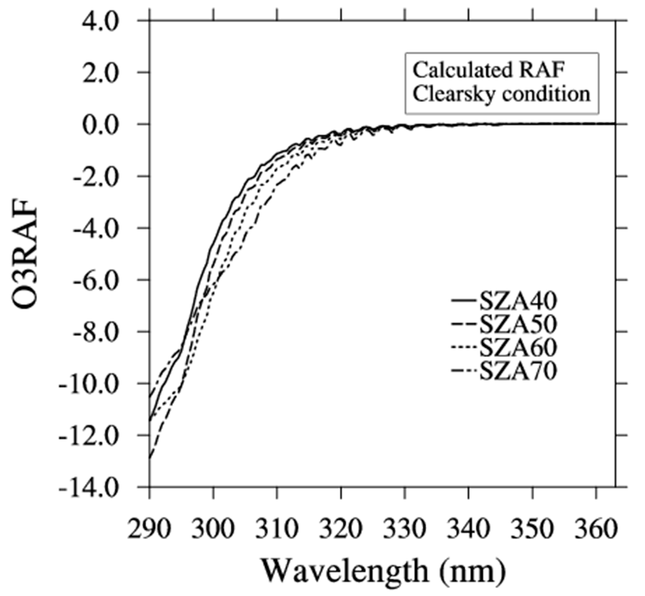
Figure 2 shows the spectral O3RAF under cloud-free conditions from the radiative transfer model (RTM) calculation with respect to SZA. In the O3RAF value with respect to SZA, the irradiance data were considered the surface albedo variation from 0.0 to 0.5. 
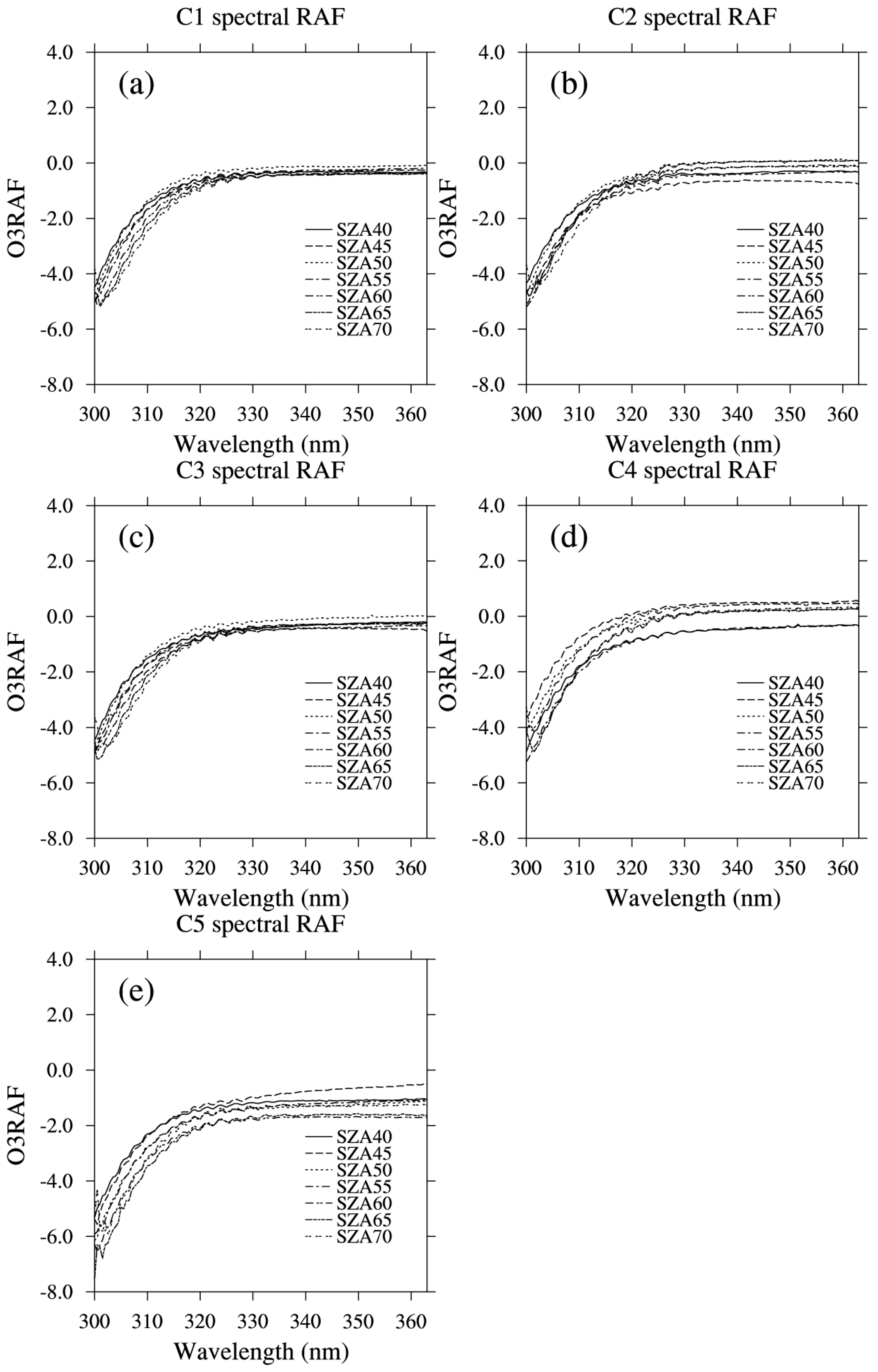
Figure 3 shows the mean O3RAF from the observational data for the C1–C5 cases. To estimate the theoretical O3RAF, the total ozone is calculated to be the range from 250 to 550 Dobson Unit (DU), which corresponds to a typical annual variation in Seoul [38,39], in 10 DU steps. Because of the spectral characteristics of the ozone absorption bands, the O3RAFs from both the RTM simulation and observations converge at 0 for wavelengths longer than 325 nm. In addition, the O3RAF at wavelengths shorter than 325 nm is theoretically estimated to be negative, indicating that the UV irradiance decreases due to increasing total ozone. In the shortwave region, the O3RAF values from both observation and simulation are negative, and they qualitatively converge at around 0 in the long-wave region. Because of the long optical path length caused by an increasing SZA, the O3RAF increases with SZA. For SZA between 40° and 70°, the O3RAF is amplified by more than 1.5 times in the spectral range of ozone absorption. Furthermore, the O3RAF decreases sharply with increasing wavelength due to the spectral characteristics of the ozone absorption band.
A quantitative bias of the O3RAF between the model and observations is found, although the shapes of the spectral variations are similar between the model and observations. The O3RAF from the RTM under clear-sky conditions sharply converges to 0.0 in the long wavelength range for all surface albedo and SZA conditions (Figure 2). However, the O3RAFs from the observations vary considerably with changing cloud and SZA conditions. The discrepancies of O3RAF at wavelengths longer than 330 nm range from −1.0 to 1.0, and the intensity of the discrepancies is amplified as the cloud conditions change. Because observation data use a loose threshold in order to ensure the number of observations for clear-sky conditions, the O3RAF error arose under a range of conditions during the long-term observations. Changes in observational conditions also affect the O3RAF in the spectral range of ozone absorption. Therefore, the O3RAF based on observation potentially includes the effects of both ozone absorption and variations in observation conditions. In addition, it is difficult to correct for spectral irradiance in the case of O3RAF based on observations.
The interactions between ozone and tropospheric scattering materials are thought to have a negligible effect on radiation, because most of the total ozone is distributed in the stratosphere, while scattering by clouds and aerosols occurs mostly in the lower troposphere. Therefore, a model-based value can be used for the reference O3RAF under clear-sky conditions (i.e., aerosol- and cloud-free conditions). Based on the O3RAF, the UV irradiance is spectrally corrected to the reference total ozone amount condition, 300 DU. 
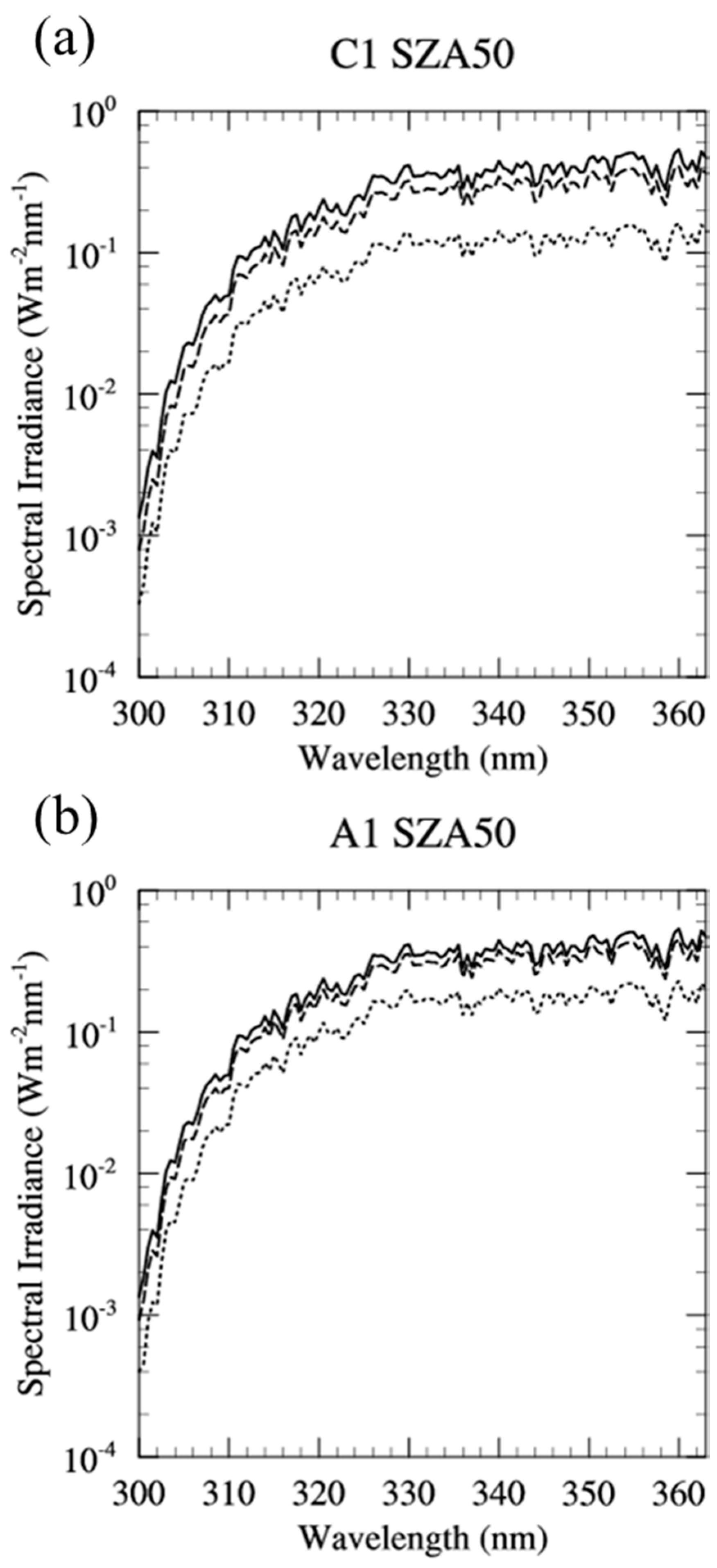
Figure 4 shows the spectral UV irradiance after correction of the total ozone amount for the C1 and A1 cases. After correction of the total ozone amount using O3RAF, the observed UV irradiance convergence is improved, especially at wavelengths shorter than 330 nm. Thus, by correcting the total ozone amount we can estimate the CMF and AMF accurately.

3.2. CMF

Figure 5 shows an example result of the spectral CMF from the RTM simulations at SZA of 40°, 50°, 60°, and 70°. Because the RTM assumes a homogeneous cloud-covered sky owing to the 1-dimensional assumption, all CMFs explain the attenuation under overcast conditions. For this reason, the theoretical CMF can be used to identify differences in observational CMF by changing the cloud thickness. The largest decreases in CMF due to the COD change are seen for a COD of 5, and the smallest for a COD of 20. In addition, the CMF value decreases at longer wavelengths for all SZA and COD conditions. In Figure 5, the difference in CMF between 300 and 360 nm is about 0.05. Table 3 shows the spectral CMF for COD values of 5, 10, 15, and 20. The spectral mean value of CMF from 300 to 360 nm at SZA of 40° is 0.80, 0.66, 0.57 and 0.50 for COD of 5, 10, 15 and 20, respectively. When the COD increases by 5, the decrease in CMF is 0.14 and 0.07 for COD of 10 and 20, respectively.
The CMF sensitivity to SZA gradually decreases with increasing SZA (Table 3). By increasing SZA in 10° increments at COD of 10, the spectrally averaged CMFs change by 0.020 at 40°, 0.019 at 50°, and 0.010 at 60° of SZA. In addition, the decrease in CMF due to SZA increases shows the spectral dependence. Previous study [30] showed that the reduction rates of broadband correction factors are insensitive for SZA change at large SZAs because of weak direct radiation intensity. Because the extinction intensity for direct radiation is affected by the spectral dependence of Rayleigh scattering, decreasing rates of CMF with SZA are larger at longer wavelengths. When the SZA changes from 40° to 50°, the decrease in the CMF is 0.003, 0.018, 0.024, and 0.028 at 300, 320, 340, and 360 nm, respectively. The optical depth due to Rayleigh scattering rapidly decreases with increasing wavelength, and the effects of cloud extinction are relatively important for determining irradiance at the surface.
Overall, the CMF has spectral sensitivities for all COD cases. Table 4 shows the spectral dependence of the CMFs, defined as the difference in CMF within the spectral range of 300 to 360 nm. Differences in CMF range from 0.032 to 0.044 for SZA of 40°, and 0.050 to 0.054 for SZA of 60°. The spectral sensitivity of the CMF is twice as large as the SZA sensitivity (compare Table 3 and Table 4). In addition, the theoretical CMFs have a peak in their spectral sensitivities at around 310 nm, which shifts to shorter wavelengths with increasing SZA. In addition, this peak point in spectral sensitivity shifts to shorter wavelengths with decreasing COD. Because Rayleigh scattering depends strongly on wavelength, the spectral decrease in CMF is intensified as optical path length increases. At shorter wavelengths, the CMF increases with increasing wavelength because of weak direct radiation and enhanced diffuse radiation [30].
In the theoretical estimation of the CMF, the spectral dependence of the CMF is a result of scattering by clouds and extinction after cloud scattering. In the real atmosphere, the CMF will also be affected by variations in cloud type, thickness, and discontinuities. 
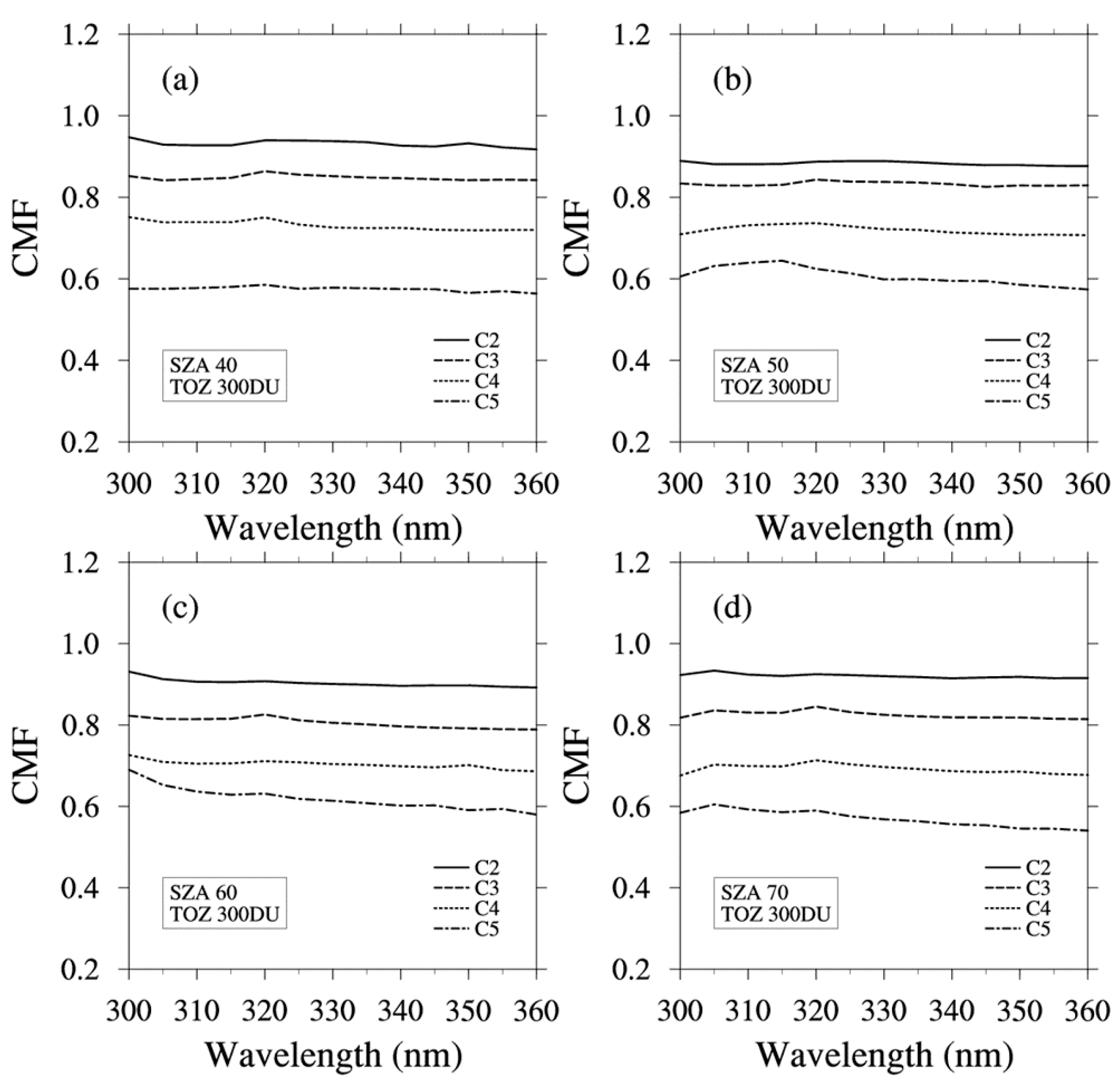
Figure 6 shows the spectral CMF with respect to SZA and cloudiness within the spectral coverage of the Brewer spectrophotometer from long-term observations. To minimize the effect of variations in instrument conditions, the CMF value is smoothed to a 5 nm resolution. With increasing cloudiness, the CMF tends to decrease for most wavelengths and SZAs. For SZAs of 40°–60°, the CMFs from 300 to 360 nm were 0.88–0.95 and 0.56–0.69 for cloudiness categories C2 and C5, respectively. All of the CMFs indicate that increasing cloud cover significantly attenuates the UV irradiance for all wavelengths and geometries. Overall, the CMF difference between C2 and C5 ranges from 26% to 41%. Furthermore, the CMF shows significant spectral dependence (Table 5). All of the cloud categories show a spectral dependence for the CMF. The spectral dependence of the CMF from 300 to 360 nm is 2.5%, 3.3%, 4.6%, and 10.0% for C2, C3, C4, and C5, respectively. Qualitatively, the spectral dependence of the CMF is related to the spectral difference in the ratio of scattering intensities between clouds and air molecules. Because the spectral dependence of the COD is less than the Rayleigh scattering, the extinction effect due to the presences of clouds is more important at longer wavelengths.
The CMF from 320 to 360 nm decreases slightly as wavelength increases, except for C2 with a SZA of 70°. The spectral CMF from the observations is similar to that from the simulation, which is based on the COD change. However the spectral CMF values and the decreasing CMF per unit wavelength are complicated within the spectral range of 300 to 320 nm. In this spectral range, the ozone absorption effect is the dominant factor in UV irradiance change. In this study, the spectral irradiance data are corrected for variation in ozone absorption by adopting the O3RAF and total ozone amount. However, there are errors associated with the measured total ozone from the Brewer spectrophotometer. The total ozone between the Brewer spectrophotometer and the Dobson spectrophotometer varied by about 5% (one standard deviation) with a 1% bias for all measurement datasets in Seoul [38]. In addition, the ZS measurement, which is the main observation method under cloudy conditions, is based on a regression equation calculated using the most recently measured DS observation under clear-sky conditions. Therefore, the total ozone from the ZS measurement varies significantly with cloud conditions due to changes in scattering. As seen in Figure 2, the O3RAF is estimated up to −6.0, which indicates that the total ozone error of 1% will lead to a CMF error of up to 0.06.

3.3. AMF

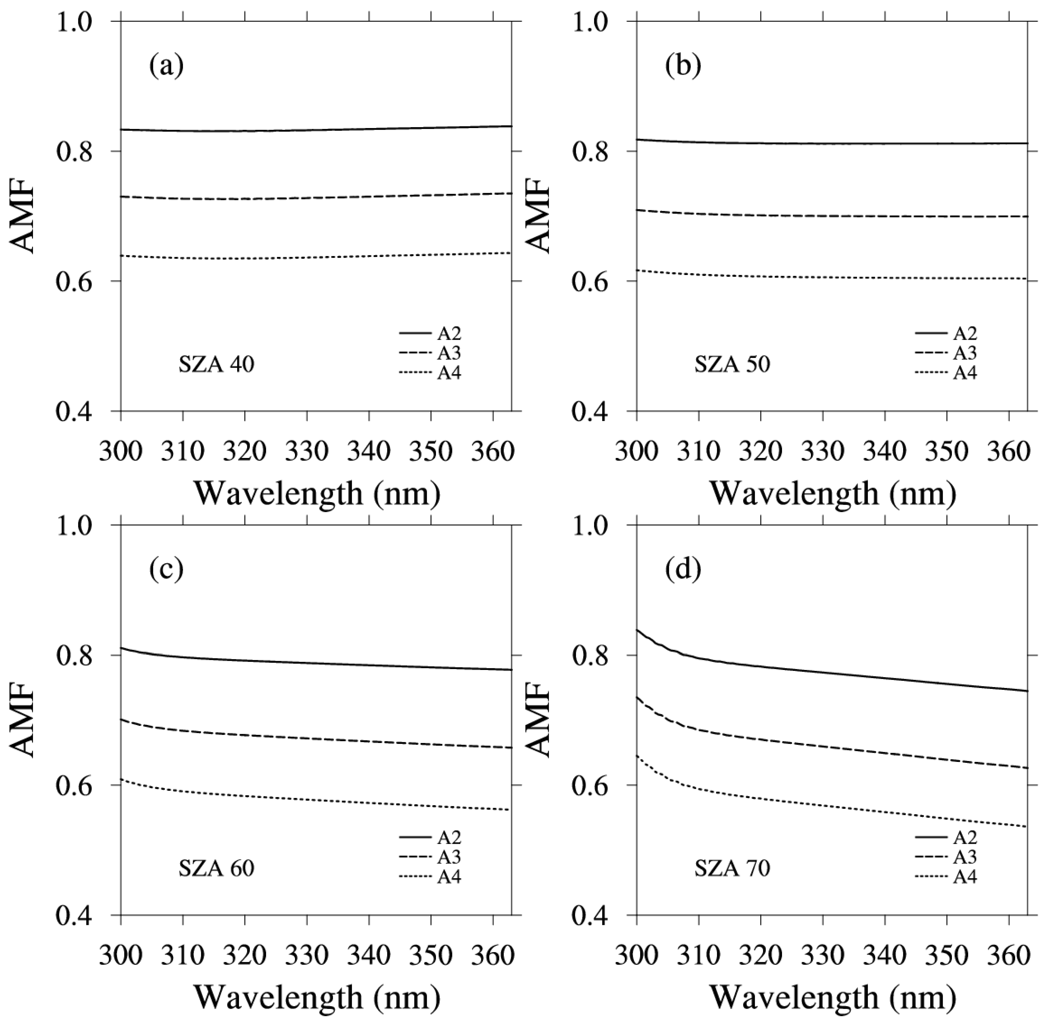
Figure 7 shows the spectral AMF with respect to AOD based on the theoretical calculation in AOD for 0.5 < AOD < 1.0 (A2), 1.0 < AOD < 1.5 (A3), and 1.5 < AOD < 2.0 (A4). When compared with the irradiance when AOD = 0.0, the AMF ranges from 0.777 to 0.866 for the A2 cases after averaging over changes in surface albedo, but the AMF decreases to 0.572–0.695 for A4, for SZA of 0°–80°. Table 6 lists the spectral AMF in AOD for A2, A3, and A4 with mean AMF and its standard deviation in AOD categories. The standard deviation is estimated by the variation of all simulated AMF value for AOD in AOD categories. Spectral mean values (standard deviations) of AMF from 300 to 360 nm at SZA of 40° are 0.833 (0.063), 0.729 (0.054), and 0.638 (0.047) in AOD category for A2, A3, and A4, respectively. When the AOD increases by 0.5 at SZA = 40°, the decrease in AMF is 0.104 and 0.091 from A2 to A3 and from A3 to A4, respectively.
The maximum and minimum AMF are summarized in Table 7 with respect to the SZA and AOD categories. The spectral dependence of the AMF is lower than that of the CMF. The AMF varies from 0.007 to 0.045 over the wavelength range in all simulation cases. Although qualitative optical characteristics of aerosol are similar to those of cloud, which have large forward scattering with small spectral dependence of optical depth, dynamic range of AOD is 10 times lower than the range of COD. For this reason, the spectral difference of the AMF is smaller than that of the CMF at the same SZA. In addition, the spectral difference of the AMF is amplified in large SZA, especially when the SZA is larger than 60°. At a SZA of 60°, the AMF difference is 4–5 times larger than for a SZA of 50°. The strong spectral contrast at large SZA is similar to that seen in CMF (Table 4). Because of the large optical path length at large SZA, the penetration depth of photons is sensitive to the wavelength change. Therefore, the AMF and CMF increase as the wavelength is reduced. In addition, the sensitivity of the spectral difference of the AMF to SZA is larger than that for the CMF, strong penetration depth effect in AMF, because the aerosol layer is assumed to be lower than the cloud layer in the RTM simulation.
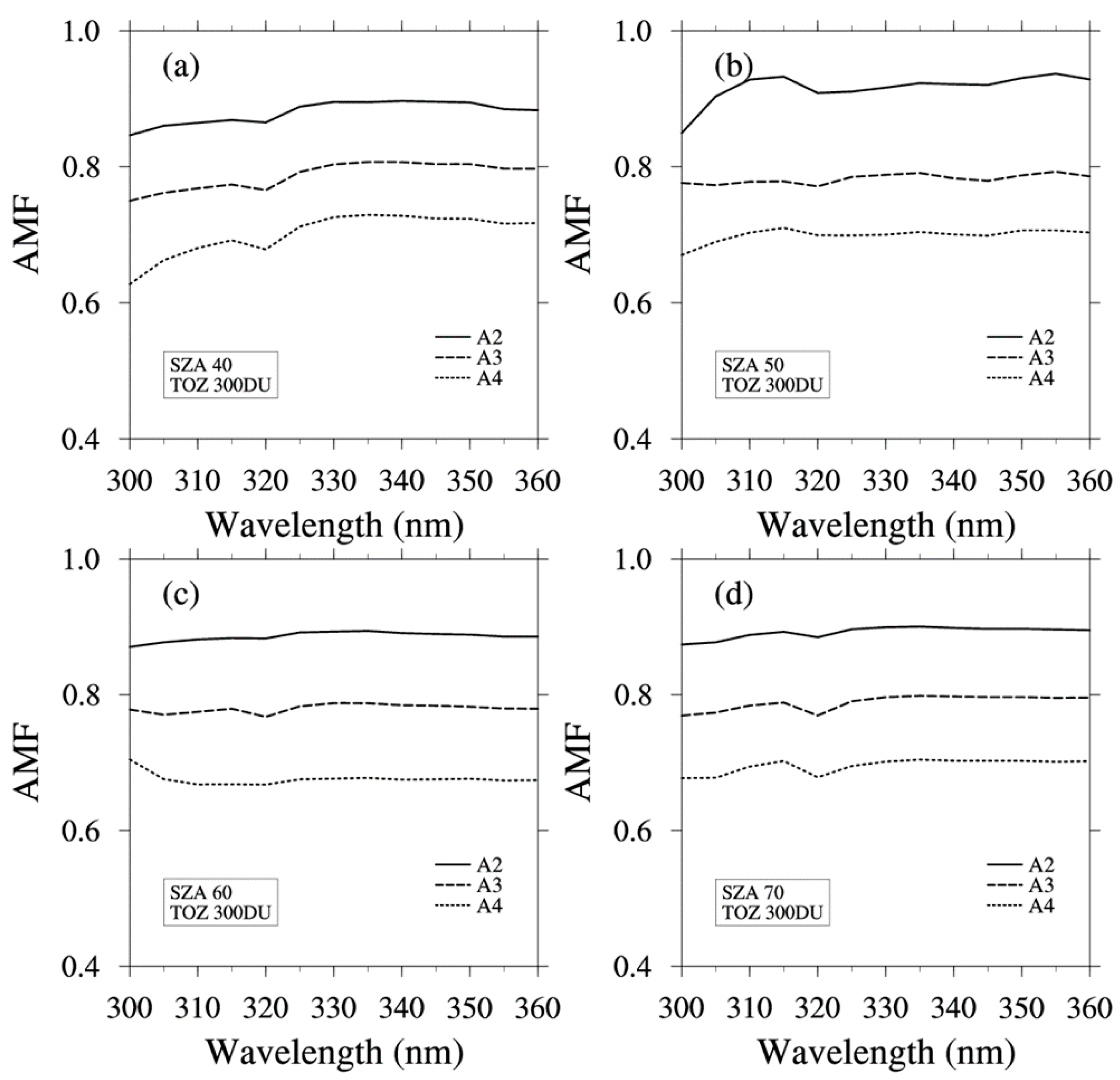
The AMF based on observations is presented in Figure 8, and AMF values are listed in Table 8. The decrease in the AMF with AOD, for SZA = 40°, is 0.09–0.10 from A2 to A3 and 0.07–0.12 from A3 to A4, similar to the theoretical AMF decreases. However, the decrease in the AMF by SZA is insignificant in all AOD categories. Similarly, the AMF shows insignificant changes over the UV spectral range, which includes variations in the AMF without a consistent spectral trend. In the CMF calculation, the spectral difference is clearly seen except in the ozone absorption range of 300–320 nm due to errors in the total ozone measurements from the Brewer spectrophotometer. Furthermore, complicated features of the spectral AMF are found in 
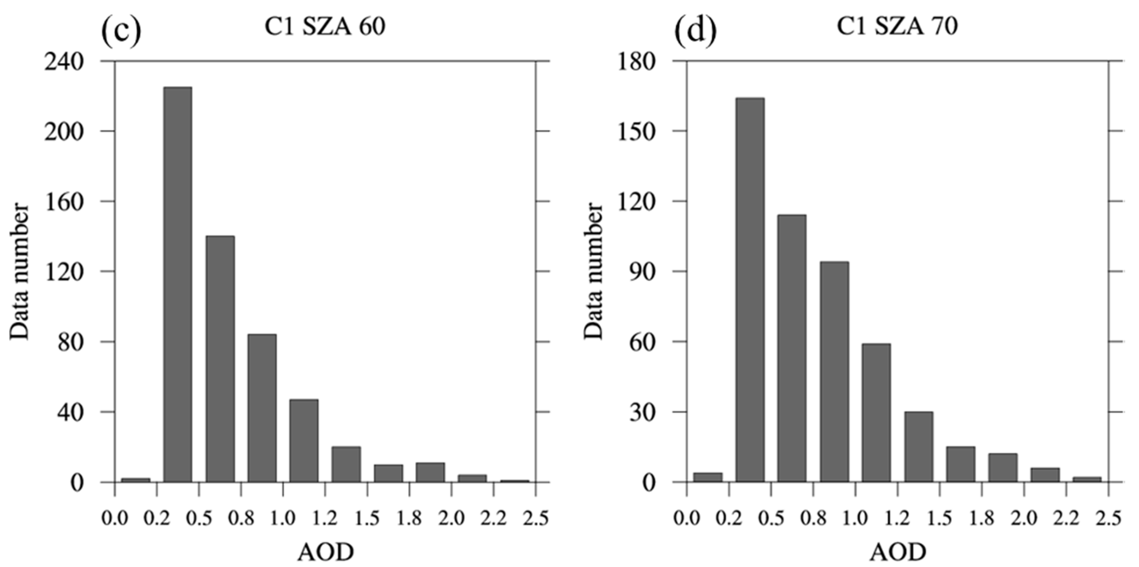
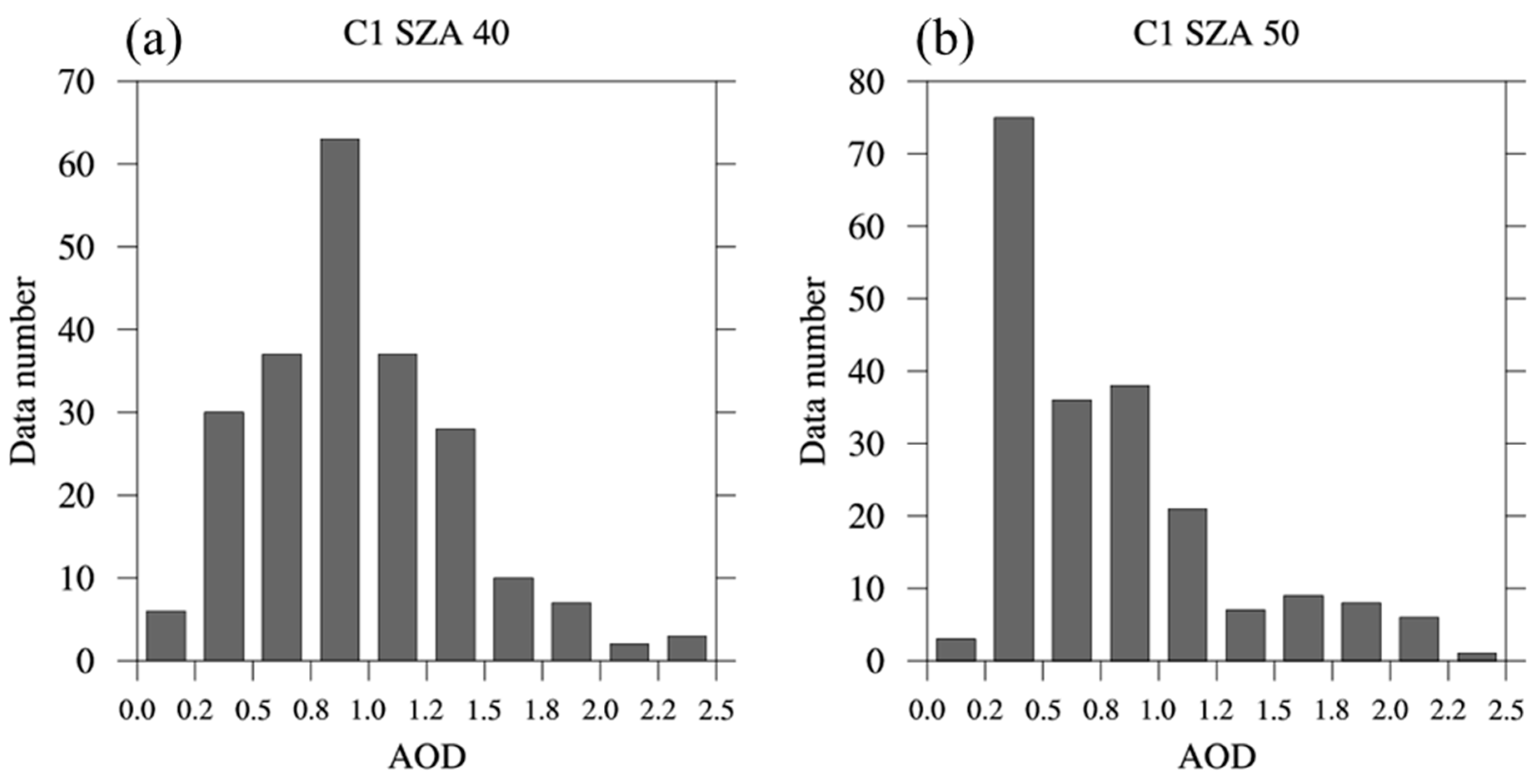
Figure 8 due to problems relating to the clear-sky assumption. The AMF from observations assumed that aerosol-free conditions have AOD < 0.5 (A1 hereafter) in order to ensure a sufficient number of observations in the calculation. From the simulation study, the AMFs for AOD < 0.5 range from 0.88 to 0.97, with dependencies on wavelength and geometry. In particular, A1 with SZA of 40° and 50° have only 35 and 71 data points, respectively, which is only around one observation per month. Therefore, referenced irradiance spectra are perturbed for SZAs of 40° and 50°, and this affects the spectral discrepancies (i.e., local maxima or minima) in the outside of spectral range of total ozone absorption. In summary, the spectral difference in AMF from observations is insignificant due to variations in the clear-sky irradiance spectrum related to the limited amount of data, in addition to the total ozone error, although the AMF shows weak spectral dependence from the RTM simulation.

4. Discussion and Conclusions

The CMF and AMF calculations are based on RTM simulations and spectral irradiance observations in the UV wavelength range for different aerosol and cloud conditions from 300 to 360 nm. Because the strong ozone absorption band affects the UV irradiance field at less than 325 nm, the O3RAF factor is used to correct the total ozone and is estimated based on the wavelength-dependent RTM results. By using the O3RAF and daily-averaged total ozone from observations, observed spectral irradiance is modified as a condition for total ozone of 300 DU to determine CMF and AMF, while accounting for ozone absorption effects.
The theoretical CMF has spectral dependencies for all cloud and geometry conditions. The spectral differences in CMFs between 300 and 360 nm are 0.032–0.054, while the decreases in the CMFs due to SZA increases range from 0.003 to 0.028 in the UV wavelength range. Because the spectral dependence of the CMF is twice as large as the sensitivity to a 10° change in SZA, the spectral dependence of CMF is considerable factors for modification of UV irradiance from the simulation result. However, the effects of cloud on the observational data depend not only on the cloud amount but also the cloud type, thickness, and discontinuities. In addition, the observed CMFs show a large spectral dependence with variations from 2.5% to 10.0% within the 300–360 nm range because of spectral differences in cloud extinction. Because of errors in the total ozone measurements, the spectral dependence of the observed CMF is identified from 320 to 360 nm.
For the AMF calculation, the data are divided into AOD categories by AOD with 0.5 intervals. The spectral mean value of the AMF at a SZA of 40° from the RTM simulation is 0.833, 0.729, and 0.638 for the A2, A3, and A4 categories, respectively. In addition, the spectral dependence of the AMF ranges from 0.007 to 0.045, which is lower than that of the CMF. The spectral difference is enhanced at large SZA, especially for SZA > 60°, due to the penetration depth of light, but the spectral dependence of the AMF is weak. The average AMF decrease with AOD, as obtained from observations, is similar to that of the RTM simulation, but the spectral dependence of the AMF is insignificant.
The observation conditions mean that the CMF and AMF calculations vary with wavelength. In the spectral range of ozone absorption, the total ozone error from the Brewer spectrophotometer affected the AMF and CMF biases. The biases due to a total ozone error of 1% lead to CMF and AMF errors of up to 0.06. For the AMF calculation, aerosol-free conditions are assumed to have an AOD < 0.5; however, the AMF value is 0.88–0.97 from the RTM simulation results for AOD < 0.5. In addition, the AMF calculation is affected by a lack of observational data for clear-sky conditions. For this reason, the reference irradiance spectra are perturbed because of losing the aerosol-free conditions in this study. Therefore, an accurate treatment of ozone absorption and obtaining a sufficiently large dataset under clear-sky conditions are essential to obtain a precise estimate of the spectral dependence of the AMF and CMF. In addition, aerosol type and optical properties are important factors in spectral AMF calculations.

Acknowledgments

This work was funded by the Korea Meteorological Administration Research and Development Program under Grant KMIPA 2015-5170.

Author Contributions

Sang Seo Park and Yun Gon Lee designed and performed the experiments; Migyoung Kim and Sang-Min Kim contributed the observation data analysis with making up the results; Hanlim Lee and Hana Lee contributed the quality assurance and check for observation data; Sang Seo Park, Migyoung Kim, and Yun Gon Lee contributed to write the manuscript.

Conflicts of Interest

The authors declare no conflict of interest.

References

  1. Bodhaine, B.A.; Wood, N.B.; Dutton, E.G.; Slusser, J.R. On Rayleigh optical depth calculations. J. Atmos. Ocean. Technol. 1999, 16, 1854–1861. [Google Scholar] [CrossRef]
  2. Bucholtz, A. Rayleigh-scattering calculations for the terrestrial atmosphere. Appl. Opt. 1995, 34, 2765–2773. [Google Scholar] [CrossRef] [PubMed]
  3. Chance, K.V.; Spurr, R.J. Ring effect studies: Rayleigh scattering, including molecular parameters for rotational Raman scattering, and the Fraunhofer spectrum. Appl. Opt. 1997, 36, 5224–5230. [Google Scholar] [CrossRef] [PubMed]
  4. Thalman, R.; Zarzana, K.J.; Tolbert, M.A.; Volkamer, R. Rayleigh scattering cross-section measurements of nitrogen, argon, oxygen and air. J. Quant. Spectrosc. Radiat. Transf. 2014, 147, 171–177. [Google Scholar] [CrossRef]
  5. Young, A.T. Rayleigh scattering. Appl. Opt. 1981, 20, 533–535. [Google Scholar] [CrossRef] [PubMed]
  6. Young, A.T. On the Rayleigh-scattering optical depth of the atmosphere. J. Appl. Meteorol. 1981, 20, 328–330. [Google Scholar] [CrossRef]
  7. Bass, A.M.; Paur, R.J. The Ultraviolet cross-sections of Ozone: I. The measurements. In Atmospheric Ozone; Springer: Dordrecht, The Netherlands, 1985; pp. 606–610. [Google Scholar]
  8. Brion, J.; Chakir, A.; Charbonnier, J.; Daumont, D.; Parisse, C.; Malicet, J. Absorption spectra measurements for the ozone molecule in the 350–830 nm Region. J. Atmos. Chem. 1998, 30, 291–299. [Google Scholar] [CrossRef]
  9. Freeman, D.E.; Yoshino, K.; Esmond, J.R.; Parkinson, W.H. High resolution absorption cross-section measurements of ozone at 195 K in the wavelength region 240–350 nm. Planet. Space Sci. 1984, 32, 239–248. [Google Scholar] [CrossRef]
  10. Griggs, M. Absorption Coefficients of Ozone in the Ultraviolet and Visible Regions. J. Chem. Phys. 1968, 49, 857. [Google Scholar] [CrossRef]
  11. Komhyr, W.D.; Mateer, C.L.; Hudson, R.D. Effective Bass-Paur 1985 ozone absorption coefficients for use with Dobson ozone spectrophotometers. J. Geophys. Res. 1993, 98, 20451–20465. [Google Scholar] [CrossRef]
  12. Molina, L.T.; Molina, M.J. Absolute absorption cross sections of ozone in the 185 to 350 nm wavelength range. J. Geophys. Res. 1986, 91, 14501–14508. [Google Scholar] [CrossRef]
  13. Yoshino, K.; Freeman, D.E.; Esmond, J.R.; Parkinson, W.H. Absolute absorption cross-section measurements of ozone in the wavelength region 238–335 nm and the temperature dependence. Planet. Space Sci. 1988, 36, 395–398. [Google Scholar] [CrossRef]
  14. Bird, R.E.; Riordan, C. Simple solar spectral model for direct and diffuse irradiance on horizontal and tilted planes at the earth’s surface for cloudless atmospheres. J. Clim. Appl. Meteorol. 1986, 25, 87–97. [Google Scholar] [CrossRef]
  15. Gueymard, C. A two-band model for the calculation of clear sky solar irradiance, illuminance, and photosynthetically active radiation at the earth’s surface. Sol. Energy 1989, 43, 253–265. [Google Scholar] [CrossRef]
  16. Madronich, S. Analytic formula for the clear-sky UV index. Photochem. Photobiol. 2007, 83, 1537–1538. [Google Scholar] [CrossRef] [PubMed]
  17. Lovengreen, C.; Fuenzalida, H.A.; Videla, L. On the spectral dependency of UV radiation enhancements due to clouds in Valdivia, Chile (39.8 S). J. Geophys. Res. 2005, 110, D14207. [Google Scholar] [CrossRef]
  18. Sabburg, J.; Wong, J. The effect of clouds on enhancing UVB irradiance at the earth’s surface: A one year study. Geophys. Res. Lett. 2000, 27, 3337–3340. [Google Scholar] [CrossRef]
  19. Sabburg, J.M.; Parisi, A.V. Spectral dependency of cloud enhanced UV irradiance. Atmos. Res. 2006, 81, 206–214. [Google Scholar] [CrossRef]
  20. Calbó, J.; González, J.A. Empirical studies of cloud effects on UV radiation: A review. Rev. Geophys. 2005, 43, RG2002. [Google Scholar] [CrossRef]
  21. Foyo-Moreno, I.; Alados, I.; Olmo, F.J.; Alados-Arboledas, L. The influence of cloudiness on UV global irradiance (295–385 nm). Agr. For. Meteorol. 2003, 120, 101–111. [Google Scholar] [CrossRef]
  22. Mateos, D.; di Sarra, A.; Meloni, D.; Di Biagio, C.; Sferlazzo, D.M. Experimental determination of cloud influence on the spectral UV irradiance and implications for biological effects. J. Atmos. Sol. Terr. Phys. 2011, 73, 1739–1746. [Google Scholar] [CrossRef]
  23. Wenny, B.N.; Saxena, V.K.; Frederick, J.E. Aerosol optical depth measurements and their impact on surface levels of ultraviolet-B radiation. J. Geophys. Res. 2001, 106, 17311–17319. [Google Scholar] [CrossRef]
  24. Kim, J.; Cho, H.K.; Mok, J.; Yoo, H.D.; Cho, N. Effects of ozone and aerosol on surface UV radiation variability. J. Photochem. Photobiol. B 2013, 119, 46–51. [Google Scholar] [CrossRef] [PubMed]
  25. López, M.L.; Palancar, G.G.; Toselli, B.M. Effect of different types of clouds on surface UV-B and total solar irradiance at southern mid-latitudes: CMF determinations at Córdoba, Argentina. Atmos. Environ. 2009, 43, 3130–3136. [Google Scholar] [CrossRef]
  26. Blumthaler, M.; Ambach, W.; Salzgeber, M. Effects of cloudiness on global and diffuse UV irradiance in a high-mountain area. Theor. Appl. Climatol. 1994, 50, 23–30. [Google Scholar] [CrossRef]
  27. Schwander, H.; Koepke, P.; Kaifel, A.; Seckmeyer, G. Modification of spectral UV irradiance by clouds. J. Geophys. Res. 2002, 107. [Google Scholar] [CrossRef]
  28. Antón, M.; Alados-Arboledas, L.; Guerrero-Rascado, J.L.; Costa, M.J.; Chiu, J.; Olmo, F.J. Experimental and modeled UV erythemal irradiance under overcast conditions: The role of cloud optical depth. Atmos. Chem. Phys. 2012, 12, 11723–11732. [Google Scholar] [CrossRef]
  29. Ogunjobi, K.O.; Kim, Y.J. Ultraviolet (0.280–0.400 μm) and broadband solar hourly radiation at Kwangju, South Korea: Analysis of their correlation with aerosol optical depth and clearness index. Atmos. Res. 2004, 71, 193–214. [Google Scholar] [CrossRef]
  30. Park, S.S.; Jung, Y.; Lee, Y.G. Spectral dependence on the correction factor of erythemal UV for cloud, aerosol, total ozone, and surface properties: A modeling study. Adv. Atmos. Sci. 2016, 33, 865–874. [Google Scholar] [CrossRef]
  31. Kerr, J.B. New methodology for deriving total ozone and other atmospheric variables from Brewer spectrophotometer direct sun spectra. J. Geophys. Res. 2002, 107. [Google Scholar] [CrossRef]
  32. Brewer, A.W.; Kerr, J.B. Total ozone measurements in cloudy weather. Pure Appl. Geophys. 1973, 106, 928–937. [Google Scholar] [CrossRef]
  33. Mayer, B.; Kylling, A. Technical note: The libRadtran software package for radiative transfer calclations—Description and examples of use. Atmos. Chem. Phys. 2005, 5, 1855–1877. [Google Scholar] [CrossRef]
  34. Mayer, B.; Seckmeyer, G.; Kylling, A. Systematic long-term comparison of spectral UV measurements and UVSPEC modeling results. J. Geophys. Res. 1997, 102, 8755–8767. [Google Scholar] [CrossRef]
  35. AFGL Atmospheric Constituent Profiles (0–120 km). Available online: http://www.dtic.mil/dtic/tr/fulltext/u2/a175173.pdf (assessed on 15 May 1986).
  36. Parisi, A.V.; Sabburg, J.; Kimlin, M.G.; Downs, N. Measured and modelled contributions to UV exposures by the albedo of surfaces in an urban environment. Theor. Appl. Climatol. 2003, 76, 181–188. [Google Scholar] [CrossRef]
  37. Kim, S.W.; Yoon, S.C.; Kim, J.; Kim, S.Y. Seasonal and monthly variations of columnar aerosol optical properties over east Asia determined from multi-year MODIS, LIDAR, and AERONET Sun/sky radiometer measurements. Atmos. Environ. 2007, 41, 1634–1651. [Google Scholar] [CrossRef]
  38. Park, S.S.; Kim, J.; Cho, H.K.; Lee, H.; Lee, Y.; Miyagawa, K. Sudden increase in the total ozone density due to secondary ozone peaks and its effect on total ozone trends over Korea. Atmos. Environ. 2012, 47, 226–235. [Google Scholar] [CrossRef]
  39. Park, S.S.; Kim, J.; Cho, N.; Lee, Y.G.; Cho, H.K. The Variations of Stratospheric Ozone over the Korean Peninsula 1985–2009. Atmosphere-KMS 2011, 21, 349–359. [Google Scholar]
Figure 1. Histogram of observation data number with respect to AOD for solar zenith angle (SZA) of: (a) 40°; (b) 50°; (c) 60°; and (d) and 70°, in C1 cases.
Atmosphere 08 00109 g001aAtmosphere 08 00109 g001b
Figure 2. Averaged spectral ozone radiation amplification factor (O3RAF) including cases for all surface albedo of 0.0 to 0.5 from the RTM calculation on clear sky condition.
Atmosphere 08 00109 g002
Figure 3. Spectral O3RAF from the observation for: (a) C1; (b) C2; (c) C3; (d) C4; and (e) C5 cases.
Atmosphere 08 00109 g003
Figure 4. Maximum (Bold), minimum (dotted), and mean (dashed) value of spectral irradiance in ultraviolet (UV) after correcting the ozone absorption based on the total ozone of 300 Dobson Unit (DU) for: (a) C1; and (b) A1 cases.
Atmosphere 08 00109 g004
Figure 5. Simulated spectral CMF for overcast sky with cloud optical depth (COD) of 5, 10, 15, and 20 at SZA of: (a) 40°; (b) 50°; (c) 60°; and (d) 70°.
Atmosphere 08 00109 g005
Figure 6. Spectral dependence of CMF of each cloud groups using calculated O3RAF at SZA of: (a) 40°; (b) 50°; (c) 60°; and (d) 70°.
Atmosphere 08 00109 g006
Figure 7. Simulated spectral AMF for A2, A3, and A4 at SZA of: (a) 40°; (b) 50°; (c) 60°; and (d) 70°.
Atmosphere 08 00109 g007
Figure 8. Spectral AMF of each AOD categories at SZA of: (a) 40°; (b) 50°; (c) 60°; and (d) 70°.
Atmosphere 08 00109 g008
Table 1. Number of observation for cloud modification factor (CMF) calculation with respect to solar zenith angle (SZA) and cloud cover (n) during the period of 2006–2010.
SZA (±2°)C1C2C3C4C5
(0 ≤ n < 2)(2 ≤ n < 4)(4 ≤ n < 6)(6 ≤ n < 8)(8 ≤ n <10)
40°206194317224101
50°21821418410731
60°56042440822385
70°498428465304129
Table 2. Number of observation for aerosol modification factor (AMF) calculation with respect to (SZA) and categories of aerosol optical depth (AOD) during the period of 2006–2010.
SZA (±2°)A1A2A3A4
(AOD < 0.5)(0.5 ≤ AOD < 1.0)(1.0 ≤ AOD < 1.5)(1.5 ≤ AOD)
40°35915921
50°71692320
60°1962076425
70°1561828032
Table 3. Spectrally averaged theoretical CMF and its geometric difference by changing 10° of SZA.
SZACOD = 5COD = 10COD = 15COD = 20
CMFDifferenceCMFDifferenceCMFDifferenceCMFDifference
40°0.7970.0220.6630.0200.5680.0170.4980.015
50°0.7740.0220.6430.0190.5510.0160.4820.014
60°0.7560.0130.6280.0100.5380.0090.4710.008
Table 4. The maximum and minimum values of theoretical CMFs and its spectral difference within the spectral range from 300 to 360 nm.
CODCMFSZA = 40°SZA = 50°SZA = 60°
5Difference0.0320.0300.053
[Minimum, Maximum][0.774, 0.806][0.756, 0.786][0.724, 0.777]
10Difference0.0380.0380.054
[Minimum, Maximum][0.637, 0.675][0.620, 0.658][0.594, 0.648]
15Difference0.0420.0390.053
[Minimum, Maximum][0.540, 0.582][0.528, 0.567][0.505, 0.558]
20Difference0.0440.0380.050
[Minimum, Maximum][0.468, 0.512][0.460, 0.498][0.440, 0.490]
Table 5. The CMF values as a function of wavelength for each cloud categories.
SZACloud CategoriesWavelength (nm)
300320340360
40°C20.950.940.930.92
C30.850.860.850.84
C40.750.750.730.72
C50.580.590.580.56
50°C20.890.890.880.88
C30.830.840.830.83
C40.710.740.710.71
C50.610.620.590.57
60°C20.930.910.900.89
C30.820.830.800.79
C40.730.710.700.69
C50.690.630.600.58
70°C20.920.920.910.92
C30.820.850.820.81
C40.680.710.690.68
C50.580.590.560.54
Table 6. Spectrally averaged theoretical AMF with its standard deviation (Stdev) for all AOD cases in AOD categories, and geometric difference of mean AMF by changing 10° of SZA.
SZA0.5 < AOD < 1.0 (A2)1.0 < AOD < 1.5 (A3)1.5 < AOD < 2.0 (A4)
AMF (Mean ± Stdev)DifferenceAMF (Mean ± Stdev)DifferenceAMF (Mean ± Stdev)Difference
40°0.833 ± 0.0630.0180.729 ± 0.0540.0250.638 ± 0.0470.028
50°0.813 ± 0.0570.0230.701 ± 0.0560.0290.607 ± 0.0470.031
60°0.789 ± 0.0710.0210.673 ± 0.0590.0230.579 ± 0.0500.020
Table 7. The maximum and minimum values of theoretical AMFs and its spectral difference within the spectral range from 300 to 360 nm.
AOD CategoriesAMFSZA = 40°SZA = 50°SZA= 60°
A2Difference0.0070.0060.032
[Minimum, Maximum][0.831, 0.838][0.812, 0.818][0.779, 0.811]
A3Difference0.0080.0100.042
[Minimum, Maximum][0.726, 0.734][0.699, 0.709][0.659, 0.701]
A4Difference0.0080.0130.045
[Minimum, Maximum][0.635, 0.643][0.604, 0.617][0.564, 0.609]
Table 8. The AMF values as a function of wavelength for each AOD categories.
SZAAOD CategoriesWavelength (nm)
300320340360
40°A20.850.860.870.90
A30.750.770.770.80
A40.630.680.680.73
50°A20.850.930.910.92
A30.780.780.770.79
A40.670.700.700.70
60°A20.870.880.880.89
A30.780.770.770.79
A40.700.670.670.68
70°A20.870.890.880.90
A30.770.780.770.80
A40.680.690.680.70

