Numerical Investigation on the Effect of Avenue Trees on PM2.5 Dispersion in Urban Street Canyons


1
College of Landscape Architecture & Arts, Northwest A&F University, Yangling 712100, China
2
Department of Building Science, School of Architecture, Tsinghua University, Beijing 100084, China
3
Beijing Key Laboratory of Indoor Air Quality Evaluation and Control, Tsinghua University, Beijing 100084, China
*
Author to whom correspondence should be addressed.
Atmosphere 2017, 8(7), 129; https://doi.org/10.3390/atmos8070129
Submission received: 14 June 2017
/
Revised: 14 July 2017
/
Accepted: 17 July 2017
/
Published: 19 July 2017
(This article belongs to the Special Issue Urban Air Pollution)
Abstract
:The Reynolds-averaged Navier-Stokes (RANS) model and revised generalized drift flux model were used to investigate the characteristics of airflow fields and PM2.5 dispersion in street canyons with a variety setting on tree crown morphologies (i.e., conical, spherical, and cylindrical), leaf area densities (LADs = 0.5, 1.5, and 2.5 m2/m3), and street canyon aspect ratios (H/W = 0.5, 1.0, and 2.0). Results were as follows: (1) airflow fields were reversed in the presence of trees and enhanced with higher LAD; (2) air velocity decreased negligibly when LAD increased from 1.5 to 2.5, but significantly when LAD increased from 0.5 to 1.5; (3) tree crown morphologies, building aspect ratios, and LADs were interrelated. The comparison of PM2.5 showed that the most critical situations in H/W = 0.5, 1.0, and 2.0 corresponded to LAD = 0.5 with a conical canopy; (4) the H/W = 1.0 and LAD = 1.5 scenario was identified as the most efficient combination for PM2.5 capture; (5) the maximum PM2.5 reduction ratio was ordered from low to high in the sequence of conical, spherical, and cylindrical canopies. At predestinated LADs and aspect ratio, Populus tomentosa with cylindrical crown morphology exhibited the best efficiency on PM2.5 capture with a reduction ratio of 75% to 85% at pedestrian height.
1. Introduction
China’s airborne particulate pollution, particularly in mega cities, is a serious environmental problem. Particulate pollution is also a social issue that has attracted increasing public concerns given its negative effects on human health [1]. Ye et al. [2] analyzed the weekly data on PM2.5 pollution and reported that PM2.5 oscillated from its highest level between mid-November and December to its lowest level from June to September. The statistical data calculated by the Beijing Municipal Environmental Monitoring Center (BJMEMC) indicated that 42 days in 2015 had serious PM2.5 pollution (12% of the full year), and the average concentration of these heavy polluted days exceeded 280 μg/m3 [3].
Urban tree planting is promoted as an effective measure for reducing particulates and mitigating air pollution. This measure is based on the underlying idea that trees can capture particulates because of their large leaf area density (LAD) and the turbulent air movement created by their structure [4]. Given the nationwide problem of air pollution, researchers have recently renewed their interest in the absorption of particulates and improvement of urban air quality by trees.
Many field experiments and wind tunnel tests have been conducted to quantify the deposition velocities and capture efficiency of trees [5,6,7,8,9,10,11]. A field measure that determined the effects of trees on nitrous oxide distribution in street canyons revealed that trees considerably affected the accumulation of transported pollutants [12]. A seasonal field investigation on six typical street canyons in Shanghai reported that PM2.5 was inversely related to the height in tree-free street canyons, while it increased at the top of street canyons with trees. Moreover, the most influential factors on the attenuation coefficient were tree canopy density, leaf area index, and wind speed [13]. The comparison of particulate deposition velocities on Pine, Yew, and Ivy showed that Pine had the maximum particulate capture capacity [14], and deposition velocities of soot particles were higher on needles than on broadleaves [15]. Several experiments have shown that coarse particles were more easily washed from leaves by rainwater [14], that is, approximately 60% of particulate deposition on foliage was washed off by rainwater, whereas the remaining 40% was observed in the wax layer of the foliage [16]. Field experiments have also demonstrated that particles smaller than 10 μm could not be washed off by rainwater [17].
As a consequence of complexity of particle dynamics in trees, full-scale field experiments are usually performed at a limited number of points at few sampling sites [18]. Moreover, controlled and replicated experiments under identical conditions are difficult and time consuming because of the nature of uncontrolled weather conditions [19]. With the rapid development of computational technologies, Computational Fluid Dynamics (CFD) has been increasingly used and adopted to simulate airflow and pollutant dispersion around buildings. In addition, CFD is certified as the preferred strategy for parametric studies on physical airflow and dispersion processes at the micro scale [20,21].
The results of numerical modeling studies have indicated that trees in built environments exerted similar effects as a solid barrier, and particle dispersion was affected by trees species, crown morphology, porosity, LADs, trees height, and tree-building distance [22]. Simulations have shown that wide streets and low building heights favored air ventilation and the removal of air pollutants within an isolated street canyon [23]. Furthermore, expanding tree crown diameters increased the particle concentration along the leeward wall of a street canyon and decreased local concentrations at the windward wall [24]. A dispersion numerical study revealed that the larger street canyon aspect ratio (H/W) corresponded to the smaller effect of trees on pollutant reduction regardless of tree morphology and arrangement, and lower air velocity resulted in more traffic-generated pollutants [25]. Similar studies indicated that trees decreased air velocity, inhibited canyon ventilation, and then increased particulates, and increasing the H/W and vegetation density led to lower ventilation and higher particles concentrations [26,27]. Buccolieri et al. [28] reported that street-level particulate dispersion relied on wind direction and H/W, and urban trees adversely affected gaseous pollutant dispersion in street canyons given their weakening effect on pedestrian level airflows. Zhang et al. [29] demonstrated that decreasing the H/W contributed to pollution dispersion in street canyons, and increasing, the aspect ratio of shallow canyons decreased NOx but increased O3 [30]. The detached eddy simulation model was applied to simulate turbulent fluid flow by using a non-commercial numerical tool based on the artificial compressibility version of the characteristic based split algorithm and the one equation Spalart-Allmaras turbulence model [31]. Another study from the same research group showed that increasing the building height impeded particulate dispersion, while higher values of approaching wind speed facilitated particulates dispersion [32]. Several studies have demonstrated that lower wind velocity produced worse effects of trees on air pollutant deposition, whereas perpendicular winds led to larger pollution concentrations in street canyons in the presence of trees [33]. The results of a large-eddy simulation of transport pollutants with H/W = 2 illustrated that the spatial variation of pollutants should be given considerable attention because of the existence of two unsteady vortices in deep urban street canyons [34]. Combining RANS equations with a dry deposition velocity model and three different wake turbulence models, the analysis on the vegetational filtration of ultrafine particles (UFP) indicated that model predictions were sensitive to the choice of wake turbulence model and certain model parameters, and thin roadside vegetation was not always effective in filtering UFP [35]. Yet another RANS simulation indicated that vegetation height and the magnitude of the micro-scale deposition velocity were the main parameters that determined whether deposition or reduction of ventilation effects prevailed [36]. Moreover, a newly published simulation study reported that vegetation with LADs = 0.5 and 1.0 weakened the ventilation efficiency of NO and NO2, but boosted the efficiency of O3 [37].
Previous studies have already appraised the clear impact of urban trees on particulates with 3D numerical models, and several studies have validated this impact on street canyons with different aspect ratios. However, these studies often used rudimentary representations of urban trees due to insufficient species-specific information, such as crown dimensions, LAD, and tree height. Moreover, the majority of previous dispersion models depicted trees as rectangular porous medium and did not consider their canopy morphologies, such as conical, cylindrical, and spherical. Furthermore, tree crown morphology and LAD are the key factors that influence the local distribution of atmospheric particles [38,39]. Providing the optimum combination of building height, road width, and tree characteristics (i.e., shape, dimensions, and LAD) in urban street canyons would considerably benefit urban design for maximizing PM capture.
Based on the RANS and revised generalized drift flux models, this study utilized the CFD code PHOENICS (Parabolic Hyperbolic Or Elliptic Numerical Integration Code Series) to evaluate the effects of relationships among the tree crown morphologies, LADs and H/W on outdoor airflows and ambient PM2.5 dispersion. A tree-free environment was also simulated, and the results were compared with the simulations under foliage conditions to identify the reduction effect of trees. The optimum combinations of the tree crown characteristics and street canyon aspect ratios were obtained via a series of simulations and comparisons.
2. Methods
2.1. Simulation Model
2.1.1. Airflow Model
The standard k-ε model was selected for airflow simulation. Vegetation was treated as a porous medium in the airflow model given the effect of vegetation canopy on airflows. Branches and trunks were approximated as leaves and canopy [40]. From an aerodynamic perspective, vegetation decreases air velocity by exerting drag forces and pressure. Therefore, the effects of vegetation on turbulent flow fields were modeled, including drag forces based on momentum equations. Turbulence production and accelerated turbulence dissipation within the canopy were also considered by the additional turbulence source terms. These equations are expressed as follows:
Continuity equation:
where ui is the spatial average velocity, and xi is the spatial coordinate.
Momentum equation:
where P is the pressure (Pa); ρ is the air density (kg/m3); Fd is the additive term for the presence of canopy resistance; veff is the effective viscosity (N s/m2) that is computed as:
where k is the turbulent kinetic energy (Nm); ε is the dissipation rate (m/s); vt is the turbulent kinetic viscosity (N s/m2); cμ is an empirical constant that is defined as 0.09 [41].
According to the conventional parameterization of the plant-airflow interaction, Fd is expressed as follows:
where S is the average velocity (m/s) and can be calculated as ; Cd is the drag coefficient induced by trees. According to previous studies, the drag coefficient can be estimated as 0.1 ≤ Cd ≤ 0.3 for most vegetation types [42]. For the tree types in this study, an average drag coefficient of Cd = 0.2 was used; α is the LAD (m2/m3), and ηα is the projection area of vegetation leaves on the vertical plane with respect to the prevailing wind direction (m2).
Considering the turbulent interactions between the plant canopy and airflow, the turbulent kinetic energy transport equation is expressed as follows:
where Gk and Gb are the generated terms for turbulent kinetic energy and buoyancy, respectively.
The additional source terms Pk and Lk in the transport equation are expressed as follows:
Similarly, given the influence of plant canopy, the kinetic energy dissipation rate equation is expressed as follows:
The additional source terms Pε and Lε in the dissipation rate equation are expressed as follows:
where σk, σε, Cε1, and Cε2 are closure constants with values of 1.0, 1.3, 1.44, and 1.92, respectively. The comparison of field data and the simulation results demonstrated that coefficients Cpε1 and Cpε2 can be set to 1.8 and 0.6, respectively [43].
2.1.2. Revised Generalized Drift Flux Model
Particles are removed from the atmosphere when they collide with foliage after any of the following processes: (1) sedimentation; (2) diffusion; (3) turbulence; (4) washout; and (5) occult deposition [4]. The Eulerian model, which treats particles as a continuum when solving the particle mass/number concentration conservation equation, has been widely used for its accuracy and convenience in modeling particle dispersion. The revised generalized drift flux model, which considers the slippage between the particle and the fluid (air) phase, is a widely used Eulerian model for particle dispersion modeling. Trees enhance gravitational sedimentation and particle deposition by turbulence diffusion, which were three-dimensionally modeled in the revised generalized drift flux model. Trees also absorb particles, and some particles may be resuspended or washed out from foliage [6], which were modeled as additional terms (Ssink and Sresuspension) in the model. Thus, the revised generalized flux model could simulate the actual urban environment comprehensively and accurately [44]. This model is expressed as follows:
In the revised generalized drift flux model, the slippage velocity of particulate matter in air (Vslip,j) could be calculated as follows:
where Vj and Vslip,j are the spatial average fluid (air) velocity and gravitational settling velocities of particulate matter in the direction j (m/s), respectively; C is the inlet particulate concentration (μg/m3); εp is the eddy diffusivity of PM (m2/s); Sc is the generated rate of the PM source (kg/(m3s)). Ssink is the mass of PM absorbed per unit vegetation volume per unit time (μg/m3), and could be calculated as Ssink = Vd × C × α; Sresuspension is the secondary pollutants from foliage per unit vegetation volume per unit time (μg/m3) [6,45], and is calculated as Sresuspension = Vr × Csink × α, Vd is the particulate deposition velocity on the foliage (m/s); Vr is the particle resuspension velocity from the foliage (m/s); Csink is the particle concentration on the foliage (μg/m3); α is LAD (m2/m3). Vpj and Vpi in Equation 12 are the average velocities of the particulate matter in the directions j and i (m/s), respectively. τp is the relaxation time of particulate matters that is calculated using Equation 14; gj is the acceleration of gravity in the direction j (m/s2); ΣFj is the entire force exerted on the particulate matter (m/s2); Smj is the momentum source of the particulate matter in the direction j (kg/(m2 s2)); μ is the molecular dynamic viscosity of air (N s/m2); ρp is the density of PM (kg/m3); dp is the diameter of PM (m); Cc is the Cunningham coefficient exerted by slippage.
2.1.3. Validation Studies
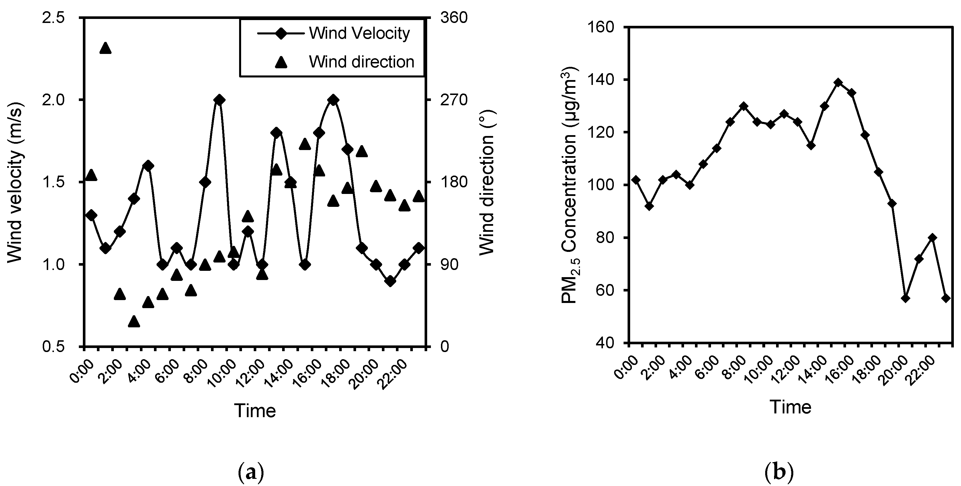
The standard k-ε and revised generalized drift flux models were compared using field measurement data from the He Qingyuan District near Tsinghua University in Beijing (39.9° N and 116.3° E). Twelve measurement points (P1–P12) were installed at the pedestrian level (1.5 m height) to monitor the impact of airflow and particle dispersion on the daily activities of citizens. Point Pw was fixed on the top of a building to measure the incoming wind velocity, wind direction, and particulate concentration at a height of 21 m (Figure 1). The test was conducted on 21 May 2016. The measurement parameters frequency, including wind velocity, wind direction and PM2.5 concentration, was set at 10 min intervals and averaged by hour (Figure 2).
Proper vegetation, buildings, and other facilities parameters should be established based on the actual environment to compare the measured data and simulation results, and validate the model accuracy. There were over 20 plants species in the green spaces. For the tractability of numerical calculations, typical species that accounted for 89.2% of the total vegetation were selected upon which to build the vegetation model. The number of trees, crown height (CH), crown diameter (CD), crown base height (CBH), and the 3D geometric crown figure were recorded. A LAI-2200C Plant Canopy Analyzer (LI-COR Inc., Lincoln, NE, USA) was used to estimate the LADs of these trees (Table 1). The three dimensions of buildings were also measured.
Models were built based on the actual district configuration. The distances of the computational domain inlet and lateral boundaries to the built area were set to 30 H, the outlet boundary was assigned to 35 H far from the built area, and the top was set at a height of 10 H from the ground, where H is the height of buildings. Thus, the size of computational domain was 1680 m in length, 1590 m in width, and 210 m in height. A second-order accurate central difference scheme was used to model the convective terms with adaptive damping to resolve non-physical oscillation. Boundary conditions were set using the mathematical equations (Equations (15)–(18)). Moreover, numerical calculations were performed on the total number of grids of 6.05 × 10⁷ (Xmin = Ymin = Zmin = 0.1 H), 1.18 × 10⁸ (Xmin = Ymin = Zmin = 0.08 H), and 4.84 × 10⁸ (Xmin = Ymin = Zmin = 0.05 H). After the grid independency testing using mathematical equations (Equations (19)–(21)), the grid convergence index (GCI) for the 6.05 × 10⁷ and 1.18 × 10⁸ grids differed by 2.72%, whereas the difference was 2.61% for 1.18 × 10⁸ and 4.84 × 10⁸ grids. Therefore, the GCI (u) differences were all less than 5%, and the grids of 1.18 × 10⁸ (Xmin = Ymin = Zmin = 0.08 H) were selected.
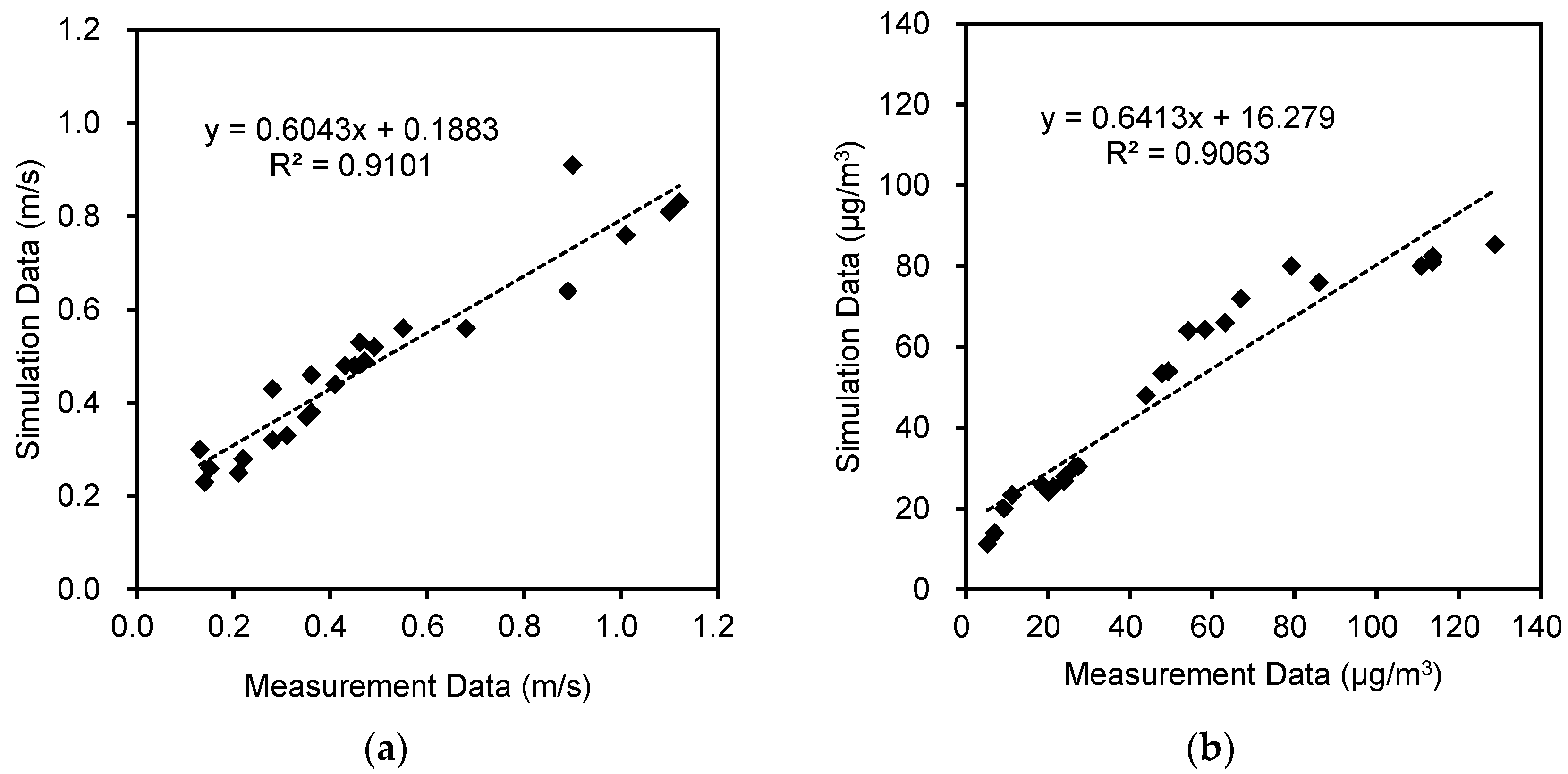
Mean values of on-site experimental measures (including air velocity and PM2.5) at 08:00–09:00 and 14:00–15:00 at point Pw were selected as the initial values for simulation. At these time periods, residuals were concentrated in outdoor activities. The average data of each point (P1 to P12) were calculated and compared with the simulation data (Figure 3).
The on-site measured and simulated data were analyzed using Microsoft Office Excel 2007 and Minitab 16.0. The scatter plots in Figure 3a,b exhibit high correlations (R2 = 0.910, R2 = 0.906) between the simulation results and the measured data. A paired t-test was used to determine if a significant difference existed between the on-site measured and simulated values (Table 2). The t-test results from the validation criteria showed that the relationships between paired differences within a 95% confidence interval. The null hypothesis illustrated that no significant difference existed between the means of the on-site measurement data and the simulation results for PM2.5 and wind velocity. Table 2 indicates that the significance value (Sig.) is greater than 0.05. Thus, no significant difference existed and the null hypothesis could not be rejected, thereby indicating the validity of the models in accurately representing the actual environment.
2.2. Numerical Simulation Setup
To investigate the effects of different aspect ratios on air flow and particulate dispersion, the building height (H) was set to 10, 20, and 40 m to correspond to H/W = 0.5 (shallow street canyons), H/W = 1.0 (symmetric street canyons), and H/W = 2.0 (deep street canyons), respectively [46]. Typical avenue trees, namely, Fraxinus pennsylvanica × F. velutina, Sophora japonica and Populus tomentosa, with conical, spherical, and cylindrical crown morphologies, respectively, were selected given their high application frequency in the central districts of Beijing. Their respective frequency values were 11.97%, 34.51%, and 12.68% [47]. A previous study reported that the common LADs of avenue trees range from 0.5 to 2.5 m2/m3 [48]. Thus, LADs of 0.5, 1.5, and 2.5 m2/m3 were selected in the simulation. We combined 27 cases with different tree crown morphologies, aspect ratios, and LADs (Figure 4).
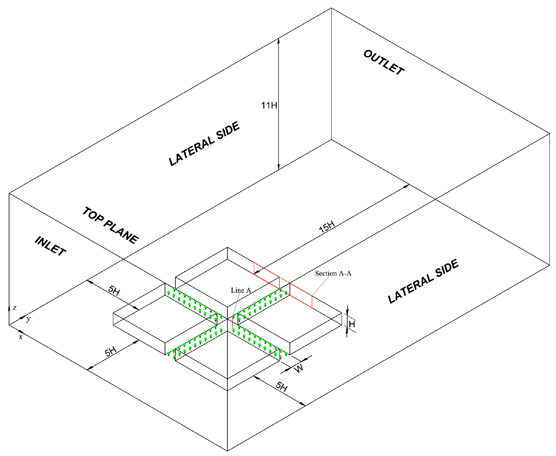
The CFD simulation computational domain was composed of two street canyons in the X-direction and one streamline canyon in the Y-direction (Figure 5). The street width, building width, and building length were 20, 100, and 100 m, respectively. The trees were modeled with the same green volumes of 10,000 m3 and planted at both sides of street canyons with a distance of 2 m from the buildings, and the CBH was set as 1 m (Table 3). In accordance with recommendations [37,49,50], the distance of the computational domain inlet to the target area was set to 5 H, and the outlet boundary was set to 15 H. A symmetry condition was imposed at the left and right lateral sides with a distance of 5 H, and the height from the ground to the top plane was set to 11 H. Section A-A was set at y = 380 m, and vertical line A was located at x = 320 m and y = 310 m.
2.3. Boundary Conditions and Grid Independence Testing
Some boundary parameters of the simulation were set to represent the typical conditions found in Beijing. The prevailing wind is northerly in the fall and winter, and the average wind velocity can reach 3.0 m/s at a height of 10 m at daytime. According to the statistical data reported by the BJMEMC, the predominant source of PM2.5 pollution in Beijing in 2015 was derived from atmospheric transmission, which accounted for 38.6% comparing with other sources (e.g., traffic, industry, and burning) [3]. This study assumed that PM2.5 was transported by wind from the outer district. Thus, the source of PM2.5 was added through the inlet. The average PM2.5 concentration (153 μg/m3) in the fall and winter of 2015 in Beijing was selected as the initial inlet concentration [3]. The discretization scheme was set as the second-order upwind, the side (sky) and the wall were set as free slip and generalized logarithmic law, respectively [51,52]. The gradient wind was considered as the inlet wind and is expressed as:
where U is the horizontal air velocity at a height of Z; U0 is the horizontal air velocity at a reference height of Z0. In the model, U0 = 3 m/s, Z = 1.5 m, and Z0 = 10 m; α is the exponent that is affected by the roughness of the ground and is set to 0.25 given that cases are investigated in the dense building complexes of urban areas [53].
The GCI was applied to evaluate the grid independence in the present simulation [54], and is calculated as follows:
where F and p are empirical constants and defined as 3 and 2, respectively; r is the ratio of fine grid to coarse grid size; u is the velocity magnitude (m/s).
For this study, three different grid sizes were generated with 1,566,234, 3,001,458 and 5,863,544 cells. The GCI (u) for the coarse and fine meshes differed by 2.72%, whereas that for fine and finest meshes differed by 2.61%. Thus, the GCIs (u) differences were all less than 5%, which indicated that the fine meshes were sufficient. The dimension of elements were selected as Xmin = Ymin = Zmin = 0.05 H, considering the consuming CPU time of the workstation.
3. Results and Discussion
3.1. Airflow Field
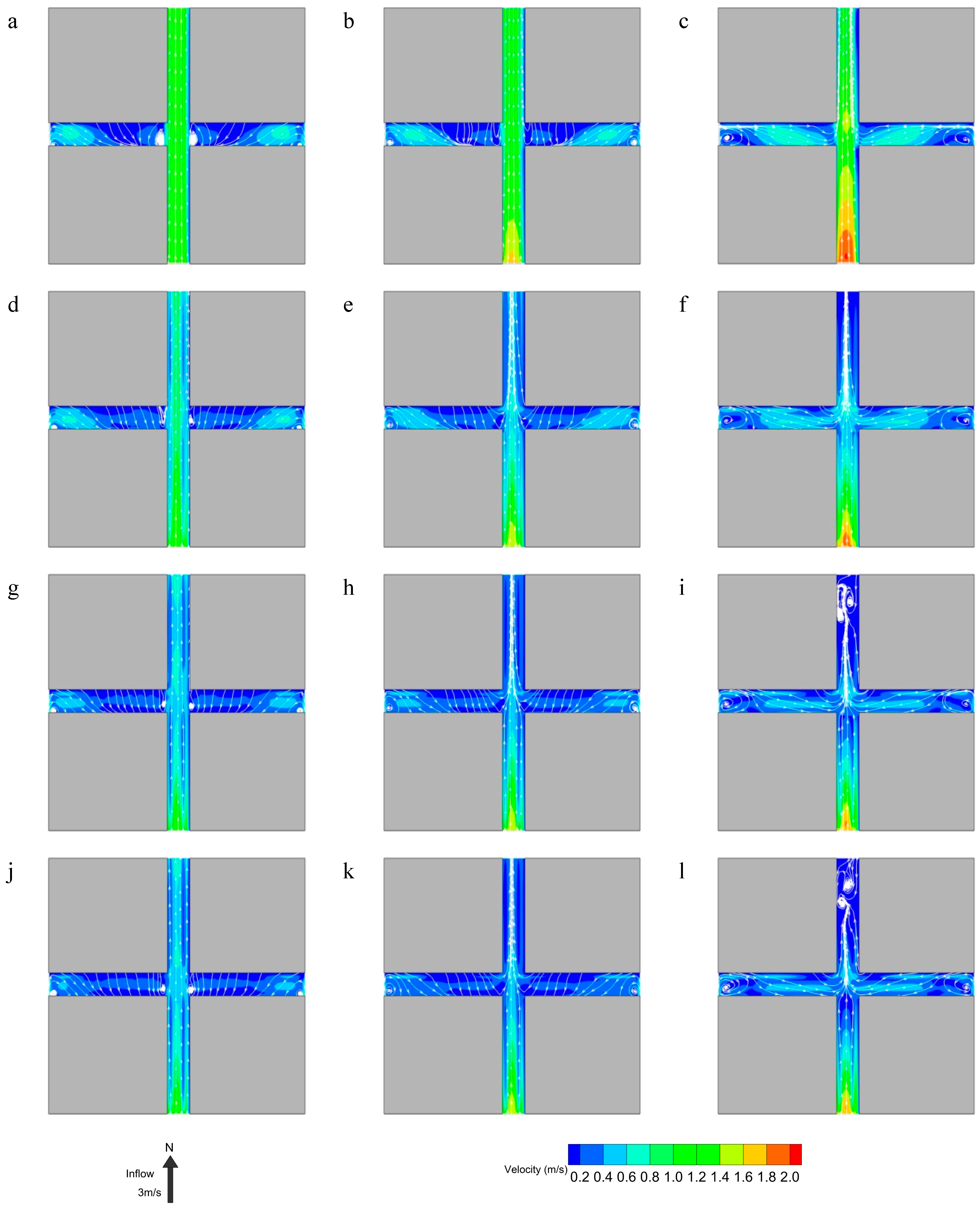
The cases with the conical crown are initially investigated. Inward airflows converge to the center of the windward street canyons, whereas the windward side airflows are obstructed. Thus, the dynamic pressure decreases (Figure 6). Meanwhile, static pressure increases because the top vortex arises. When H/W = 0.5, two vortices appear at either side of the crossroads. The vortices are smaller for cases where LAD = 0.5 than those for tree-free cases (LAD = 0). Compared with cases of LAD = 0.5, conditions are similar between cases of LADs = 1.5 and 2.5. However, smaller portal-type vortices appear in airflows on the stream-wise street in a direction from the outward street canyon to the leeward street canyon. Trees decrease airflow momentum and strengthen reverse airflow direction as LAD increases. In LAD = 1.5 cases, outward flows dominate along the street canyons. This effect is stronger in LAD = 2.5 cases. Moreover, airflow is reversed at the stream-wise street near the edge of the street canyon in LAD = 1.5 cases because the decrease in momentum in this scenario is more than that in LAD = 0.5 cases. Increasing LAD to 2.5 causes significant reverse flow at the stream-wise street and decreases air velocity. The LAD = 1.5 cases show that the flow within canyons originates from the outward street canyon to the stream-wise street for the tree-free case with small portal-type vortices. In LAD = 0.5 scenarios, trees resist flow and change its direction, thereby encountering streamlines within canyons where low airflows accumulate at both sides of the crossroad. In LAD = 1.5 cases, the flow direction within canyons is completely reversed, and airflows occur from the stream-wise street to the outward street canyons, causing the uniform distribution of air velocity.
In cases where H/W = 1.0, the convergence in the windward street canyon is enhanced and the portal-type vortices of the leeward street canyon weaken with the increasing LAD. In cases where LAD = 0.5, reverse flow at the stream-wise street and the change of the flow direction within the left-up and right-down canyons conduct lower airflows along the street canyons. The flow field where LAD = 1.5 creates a uniform wind field, and trees ensure maximize momentum and reduce air velocity in the LAD = 2.5 case (Figure 6h,k).
In H/W = 2.0 simulations, the convergence in the windward street canyon where LAD = 0.5 is stronger than that in the tree-free case. Two vortices (top-right is clockwise and the bottom-left is anticlockwise) appear in the windward street canyon near its edge because of the effects of trees on air velocity and kinetic energy where LADs = 1.5 and 2.5. The comparison of the H/W = 1.0 and H/W = 2.0 cases shows that the portal-type vortices are weak, whereas the effect of convergence is strong with the same LAD, due to the airflow-guiding effect of buildings in the H/W = 2.0 simulation.
As indicated in H/W = 2.0 scenarios with the spherical canopy, a contraction of streamlines appears at the center of windward street canyons in LAD = 0.5. An anticlockwise vortex appears near the constringency position, and airflow is reversal in the outlet area of LAD = 1.5. In the LAD = 2.5 case, two similarly aligned vortices are formed at a slightly downward constringency position, where the left vortex is anticlockwise and the other vortex is clockwise. Two small vortices appear downward of the crossroad within the windward street canyon in the H/W = 1.0 scenario, where the left (right) vortex is clockwise (anticlockwise) in the LAD = 2.5 case. Two more vortices form on the windward street canyon near the outlet areas where H/W = 2.0 compared with that where H/W = 1.0. Meanwhile, where H/W = 2.0 with a cylindrical canopy, the convergence of streamlines within the windward street canyon near the outlet areas is stronger than that of instances with spherical canopy. The downward constringency position has two similarly aligned vortices, where the left is clockwise and the right is anticlockwise. Reversal airflows also appear at the outlet. Where LADs = 1.5 and 2.5, the vortices with a downward position are visibly larger than those where LAD = 0.5. The same tendency is observed in LAD = 2.5 with a spherical canopy.
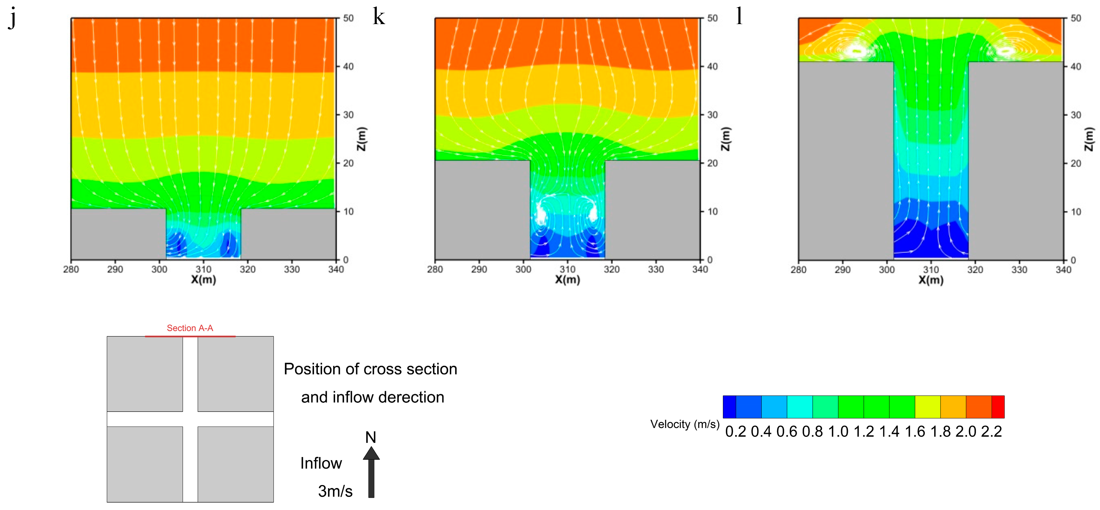
Figure 7 depicts the air velocity and streamline fields with conical canopy at y = 380 m which is shown as section A-A in Figure 5. Adding trees increases the reverse flow in the street canyon and the reduction in wind velocity. The distribution of wind fields becomes uniform as H/W increases. Air velocity increases slowly in the street canyon accompanied by high H/W. Upward flow starts from top to bottom in the tree-free scenario where H/W = 0.5. When H/W = 1.0, two parallel vortices appear in the street canyon (the left vortex is counterclockwise and the right is clockwise), and upward and downward airflows meet at approximately z = 15 m. For H/W = 2.0, two vortices (the left vortex is counterclockwise and the right is clockwise) appear at the top of the buildings in the street canyon. The analysis of cases where LAD = 0.5 indicates that upward flow, which starts from top-right to bottom-left, forms a small vortex in H/W = 0.5. Trees change the flow field, and the downward and upward flows meet at the top of the building (z = 20 m), thereby making the two-sided airflow move downwards and the middle airflow move upward. Thus, four horizontally aligned counter rotating vortices appear in the street canyon (Figure 7e). For H/W = 2.0, the airflow moves from bottom to top, and two aligned vortices appear near the building top. In cases where LADs = 1.5 and 2.5, the upward flow starts from top-right to bottom-left and forms no vortex for H/W = 0.5. Compared with LAD = 0.5, in H/W = 1.0, the aligned vortices become smaller (LAD = 1.5) or even disappear (LAD = 2.5).
As manifested when H/W = 0.5 with a spherical canopy, airflow fields of spherical and conical canopies are similar. For H/W = 1.0 simulations, no vortex forms on the upper space of the building. For LAD = 0.5, the airflow moves from the upper street to the canyon and converges from the two sides to the center. A right-clockwise vortex forms on the street canyon where LAD = 1.5, and an obvious convergence in the lower canyon is observed where LAD = 2.5. In the H/W = 2.0 scenario with a spherical canopy, no vortex forms in the canyon compared with that in LAD = 0.5 with a conical canopy. Meanwhile, for the cylindrical canopy, the air velocity and distribution of the flow fields at H/W = 0.5 and 2.0 are similar to those of the spherical crown. However, when H/W = 1.0, two weak vortices form where LAD = 0.5. Additionally, the airflow convergence effect is subtle in the lower layer of the LADs = 1.5 and 2.5 scenarios when compared with the spherical canopy.
Air velocity at pedestrian height (1.5 m) with various LADs and tree shapes decreases as LAD increases (Figure 8). However, as LAD increases from 1.5 to 2.5, the wind velocity reduction becomes negligible (ranging from 0.02 m/s to 0.03 m/s). Meanwhile, the reduction becomes considerable as LAD increases from 0.5 to 1.5 with values of 0.11, 0.08, and 0.11 m/s for H/W = 0.5, 1.0 and 2.0, respectively. The reduction in wind velocity is higher for spherical and cylindrical canopies than that for the conical canopy. When LAD increases from 0.5 to 1.5, the reductions in wind velocity with the spherical canopy are 0.08, 0.08, and 0.14 m/s, respectively, and that with the cylindrical canopy are 0.09, 0.09, and 0.12 m/s for H/W = 0.5, 1.0 and 2.0, respectively.
3.2. Particulate Matter Dispersion
The pedestrian-level PM2.5 distributions decrease within windward street canyons with a conical canopy as the aspect ratio increases towards tree-free cases (Figure 9). The decrease of PM2.5 follows the descending order of H/W = 1.0, H/W = 0.5, and H/W = 2.0 for LAD = 0.5. LADs = 1.5, and 2.5 cases have the similar trajectory. The increase in LAD from 0.5 to 1.5 considerably decreases PM2.5. The decreases are negligible when LAD increases from 1.5 to 2.5. Similar tendencies are observed for H/W = 1.0 and 2.0 cases compared with H/W = 0.5 cases.
The cylindrical canopy has the strongest effect on reducing PM2.5, followed by the spherical canopy, then the conical canopy with the weakest capability at the same H/W and LADs. A similar tendency is observed for PM2.5 in windward street canyons as H/W increases. However, in the leeward street canyons, concentration decreases as H/W increases in the spherical canopy compared with the conical canopy. PM2.5 decreases as LAD increases in the same H/W scenario. Similar tendencies are observed for the cylindrical canopy compared with those for the spherical canopy.
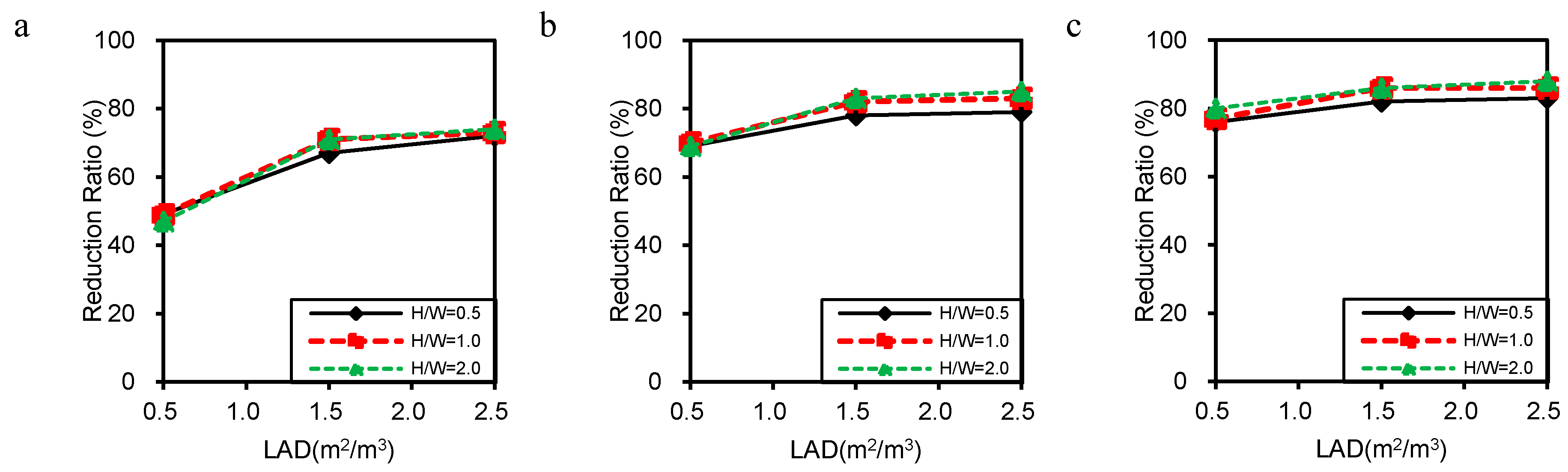
The average concentrations with and without trees at the pedestrian level are calculated to determine particulate reduction efficiency. Figure 10 depicts the attenuation coefficient in average concentrations versus LADs for the three tree canopies. The attenuation coefficient is expressed as:
where ω is the attenuation coefficient, which indicates the reduction capability of trees for particulate matter. Cave,tree-free and Cave represent the average concentration at the pedestrian level in target areas in the tree and tree-free scenarios, respectively.
The reduction ratio of average concentrations increases with LADs (Figure 10). However, the change is insignificant as H/W increases for the same tree shape. The reduction is clear as LAD increases from 0.5 to 1.5 but negligible as LAD increases from 1.5 to 2.5. As LAD increases from 0.5 to 2.5, the range of the reduction ratio is 45% to 75% for the conical canopy, 65% to 80% for the spherical canopy and 75% to 85% for the cylindrical canopy.
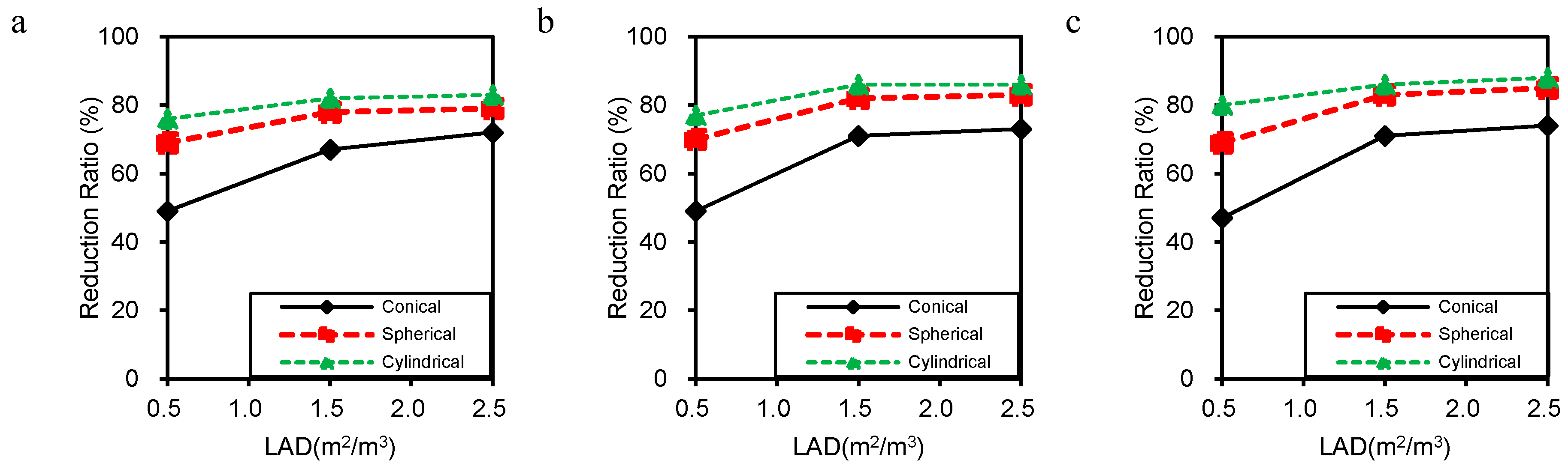
Figure 11 shows the attenuation coefficient in average PM2.5 versus LADs under the three aspect ratios, and the maximum reduction ratio ranked lowest to highest in the order of conical, spherical and cylindrical canopies. The reduction ratio obviously increases in the conical canopy and remains at approximately 80% in the cylindrical canopy.
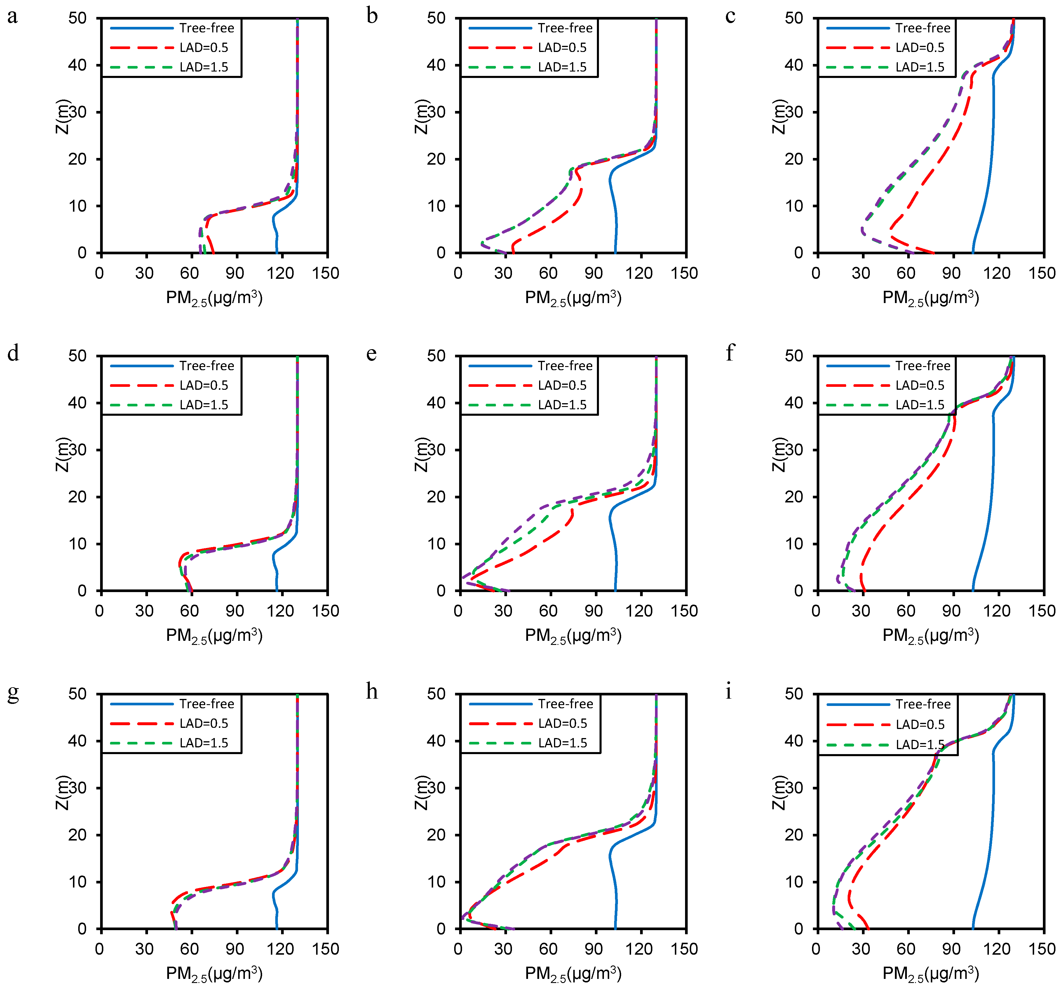
PM2.5 visibly decreases and the minimum values appear near the canopy range for tree-planted cases compared with the tree-free scenario because of the aerodynamic and deposition effects of trees (Figure 12). PM2.5 initially decreases with tree canopy height (2 m to 7 m) and then gradually increases with height. Subsequently, the values suddenly increase at the top of the buildings. The initial PM2.5 concentrations are lowest in the cylindrical canopy, followed by those in the spherical and conical canopies in H/W = 0.5 scenarios. Concentrations decrease to approximately 10 μg/m3 near the canopy in the spherical and cylindrical crowns and decrease rapidly as the height increases in the canopy where H/W = 1.0. The three canopies have similar initial PM2.5 concentrations of 30 μg/m3 in H/W = 1.0 scenarios. The values reach 4 μg/m3 and 15 μg/m3 at the height of the tree canopies with spherical and cylindrical crowns, respectively. For H/W = 2.0, spherical and cylindrical canopies have similar initial concentrations. However, the effect becomes more significant as the height increases and the concentration approximately decreases to 10 μg/m3 at the conical canopy height (2 m to 7 m). In the cases of the three canopy types, the reduction ratio is subtle with the increase in LAD from 1.5 to 2.5. As a result, where H/W = 1.0 and LAD = 1.5 is the most efficient combination for reducing the pedestrian-level PM2.5 in street canyons.
This study demonstrated that the presence of trees caused a significant reduction in PM2.5 with parallel wind to the street canyons. However, some research reported the opposite, that is, trees led to an increase in concentrations for parallel wind, such as in Gromke et al.’s wind tunnel experiment [55], and the simulation performed by Wania et al. using the ENVI-met model [26]. The CFD model used in our study resembles the wind tunnel experiment that supports this increasing effect. However, the increasing effect in the wind tunnel experiment is due to the fact that the presence of trees reduces the ventilation of the street and the emissions are located within the street at the ground level. Then, the concentration increases in this case in comparison with a tree-free street. As for the numerical study using the ENVI-met model, the turbulence and the following particle movement are traffic-induced, whereas the current study assumed that the particles are transported by the wind from the inlet.
4. Conclusions
In this study, the RANS and revised generalized drift flux models were used to analyze the effects of the tree crown morphology, LAD, and aspect ratio on airflows and PM2.5 dispersion in street canyons. Numerical simulations were conducted for cases with conical, cylindrical, and spherical tree crown morphologies in four scenarios, namely, a tree-free scenario and LADs of 0.5, 1.5, and 2.5 scenarios, with aspect ratios of 0.5, 1.0, and 2.0. The results reflected the significant impacts of site planning and tree planting design on particulate pollutants around street blocks in urban areas. The following conclusions can be drawn from the results:
(1) Trees act as a momentum sink, by reversing the airflows. Higher LAD augments reversal flow and decreases air velocity. Scenarios with high aspect ratios exhibit significant reductions in air velocity at the pedestrian level. The average air velocity decreases with increasing LAD. The air velocity reduction is negligible when LAD increases from 1.5 to 2.5, but significant when LAD increases from 0.5 to 1.5.
(2) PM2.5 distribution depends on airflow fields with higher PM2.5 observed whereas the streamlines converge. The comparison of contours shows that the most critical situations in H/W = 0.5, 1.0, and 2.0 correspond to LAD = 0.5 with a conical canopy. The maximum reduction ratio ranked lowest to highest in order of conical, spherical, and cylindrical canopies. Therefore, tree crown morphology plays a significant role in the design of street geometry with the aim of decreasing PM2.5.
(3) After a series of comparisons, the H/W = 1.0 and LAD = 1.5 scenario is identified as the optimal combination for reducing pedestrian-level PM2.5 concentrations. Moreover, Populus tomentosa with cylindrical canopy has the greatest capability to reduce PM2.5 with predestinated LADs and aspect ratios in urban street canyons.
This research provides an effective guide for the design of tree-planted avenues for a comfortable and healthy environment in urban areas. Among the limitations posed by the present research, the simulation study only utilized typical meteorological data in Beijing. Worse climate situations with high PM2.5 have recently occurred in Beijing. Thus, further field experiments and numerical simulations should be conducted to address these scenarios with further research. Another limitation is that this study assumed that the deposition velocity on foliage is constant. Moreover, the revised generalized drift flux model did not include solar radiation and convective heat transfer between trees and the environment. Thus, an interesting objective for future study is the evaluation of more complex, but realistic conditions to improve the prediction accuracy of numerical simulation for actual environments.
Acknowledgments
This study is supported by the National Natural Science Foundation of China (No.51561135001 and No. 51638003) and the Innovative Research Groups of the National Natural Science Foundation of China (No. 51521005).
Author Contributions
Bo Hong and Borong Lin conceived and designed the experiments; Hongqiao Qin performed the experiments; Bo Hong and Hongqiao Qin analyzed the data; Bo Hong wrote the paper.
Conflicts of Interest
The authors declare no conflict of interest.
References
- Chen, Y.; Ebenstein, A.; Greenstone, M.; Li, H. Evidence on the impact of sustained exposure to air pollution on life expectancy from China’s Huai River policy. Proc. Natl. Acad. Sci. USA 2013, 110, 12936–12941. [Google Scholar] [CrossRef] [PubMed]
- Ye, B.; Ji, X.; Yang, H.; Yao, X.; Chan, C.K.; Cadle, S.H.; Chan, T.; Mulawa, P.A. Concentration and chemical composition of PM2.5 in Shanghai for a 1-year period. Atmos. Environ. 2003, 37, 499–510. [Google Scholar] [CrossRef]
- Beijing Municipal Environmental Monitoring Center (BMEMC). Real-Time Air Quality in Beijing. Available online: http://www.bjmemc.com.cn (accessed on 25 January 2016).
- Beckett, K.P.; Freer-Smith, P.H.; Taylor, G. Urban woodlands: Their role in reducing the effects of particulate pollution. Environ. Pollut. 1998, 99, 347–360. [Google Scholar] [CrossRef]
- Beckett, K.P.; Freer-Smith, P.H.; Taylor, G. Particulate pollution capture by urban trees: Effect of species and wind speed. Glob. Chang. Biol. 2000, 6, 995–1003. [Google Scholar] [CrossRef]
- Ould-Dada, Z.; Baghini, N.M. Resuspension of small particles from tree surfaces. Atmos. Environ. 2001, 35, 3799–3809. [Google Scholar] [CrossRef]
- Ould-Dada, Z. Dry deposition profile of small particles within a model spruce canopy. Sci. Total Environ. 2002, 286, 83–96. [Google Scholar] [CrossRef]
- Freer-Smith, P.H.; Khatib-El, A.A.; Taylor, G. Capture of particulate pollution by trees: A comparison of species typical of semi-arid areas (Ficus nitida and Eucalyptus globulus) with European and North American species. Water Air Soil Pollut. 2004, 155, 173–187. [Google Scholar] [CrossRef]
- Freer-Smith, P.H.; Beckett, K.P.; Taylor, G. Deposition velocities to Sorbus aria, Acer campestre, Populus deltoids × trichocarpa ‘Beaupré’, Pinus nigra and × Cupressocyparis leylandii for coarse, fine and ultra-fine particles in the urban environment. Environ. Pollut. 2005, 133, 157–167. [Google Scholar] [CrossRef] [PubMed]
- Sæbø, A.; Popek, R.; Nawrot, B.; Hanslin, H.M.; Gawronska, H.; Gawronski, S.W. Plant species differences in particulate matter accumulation on leaf surfaces. Sci. Total Environ. 2012, 427–428, 347–354. [Google Scholar] [CrossRef] [PubMed]
- Moria, J.; Hanslinc, H.M.; Burchi, G.; Sæbø, A. Particulate matter and element accumulation on coniferous trees at different distances from a highway. Urban For. Urban Green. 2015, 14, 170–177. [Google Scholar] [CrossRef]
- Salmond, J.A.; Williams, D.E.; Laing, G.; Kingham, S.; Dirks, K.; Longley, I.; Henshaw, G.S. The influence of vegetation on the horizontal and vertical distribution of pollutants in a street canyon. Sci. Total Environ. 2013, 443, 287–298. [Google Scholar] [CrossRef] [PubMed]
- Jin, S.; Guo, J.; Wheeler, S.; Kan, L.; Che, S. Evaluation of impacts of trees on PM2.5 dispersion in urban streets. Atmos. Environ. 2014, 99, 277–287. [Google Scholar] [CrossRef]
- Przybysz, A.; Sæbø, A.; Hanslin, H.M.; Gawrońskia, S. Accumulation of particulate matter and trace elements on vegetation as affected by pollution level, rainfall and the passage of time. Sci. Total Environ. 2014, 481, 360–369. [Google Scholar] [CrossRef] [PubMed]
- Hwang, H.J.; Yook, S.J.; Ahn, K.H. Experimental investigation of submicron and ultrafine soot particle removal by tree leaves. Atmos. Environ. 2011, 45, 6987–6994. [Google Scholar] [CrossRef]
- Popek, R.; Gawrońska, H.; Wrochna, M.; Gawroński, S.W.; Sæbø, A. Particulate matter on foliage of 13 woody species: Deposition on surfaces and phytostabilisation in Waxes-a 3-Year Study. Int. J. Phytoremediat. 2013, 15, 245–256. [Google Scholar] [CrossRef] [PubMed]
- Terzaghi, E.; Wild, E.; Zacchello, G.; Cerabolini, B.E.L.; Jones, K.C.; Di Guardo, A. Forest filter effect: Role of leaves in capturing/releasing air particulate matter and its associated PAHs. Atmos. Environ. 2013, 74, 378–384. [Google Scholar] [CrossRef]
- Montazeri, H.; Blocken, B. CFD simulation of wind-induced pressure coefficients on buildings with and without balconies: Validation and sensitivity analysis. Build. Environ. 2013, 60, 137–149. [Google Scholar] [CrossRef]
- Schatzmann, M.; Leitl, B. Issues with validation of urban flow and dispersion CFD models. J. Wind Eng. Ind. Aerodyn. 2011, 99, 169–186. [Google Scholar] [CrossRef]
- Britter, R.; Schatzmann, M. Background and justification document to support the model evaluation guidance and protocol. Int. J. Environ. Pollut. 2007, 44, 139–146. [Google Scholar]
- Gousseau, P.; Blocken, B.; Stathopoulos, T.; Van-Heijst, G.J.F. CFD simulation of near-field pollutant dispersion on a high-resolution grid: A case study by LES and RANS for a building group in downtown Montreal. Atmos. Environ. 2011, 45, 428–438. [Google Scholar] [CrossRef] [Green Version]
- Gallagher, J.; Baldauf, R.; Fuller, C.H.; Kumar, P.; Gill, L.W.; McNabola, A. Passive methods for improving air quality in the built environment: A review of porous and solid barriers. Atmos. Environ. 2015, 120, 61–70. [Google Scholar] [CrossRef]
- Chan, T.L.; Dong, G.; Leung, C.W.; Cheung, C.S.; Hung, W.T. Validation of a two-dimensional pollutant dispersion model in an isolated street canyon. Atmos. Environ. 2002, 36, 861–872. [Google Scholar] [CrossRef]
- Gromke, C.; Ruck, B. Influence of trees on the dispersion of pollutants in an urban street canyon-Experimental investigation of the flow and concentration field. Atmos. Environ. 2007, 41, 3287–3302. [Google Scholar] [CrossRef]
- Buccolieri, R.; Gromke, C.; Sabatino, S.D.; Ruck, B. Aerodynamic effects of trees on pollutant concentration in street canyons. Sci. Total Environ. 2009, 407, 5247–5256. [Google Scholar] [CrossRef] [PubMed]
- Wania, A.; Bruse, M.; Blond, N.; Weber, C. Analysing the influence of different street vegetation on traffic-induced particle dispersion using microscale simulations. J. Environ. Manag. 2012, 94, 91–101. [Google Scholar] [CrossRef] [PubMed]
- Vos, P.E.J.; Maiheu, B.; Vankerkom, J.; Janssen, S. Improving local air quality in cities: To tree or not to tree? Environ. Pollut. 2013, 183, 113–122. [Google Scholar] [CrossRef] [PubMed]
- Buccolieri, R.; Salim, S.M.; Leo, L.S.; Sabatino, S.D.; Chan, A.; Ielpo, P.; Gennaro, G.; Gromke, C. Analysis of local scale tree-atmosphere interaction on pollutant concentration in idealized street canyons and application to a real urban junction. Atmos. Environ. 2011, 45, 1702–1713. [Google Scholar] [CrossRef]
- Zhang, Y.; Gu, Z.; Lee, S.; Fu, T.M.; Ho, K.F. Numerical simulation and in situ investigation of fine particle dispersion in an actual deep street canyon in Hong Kong. Indoor Built Environ. 2011, 20, 206–216. [Google Scholar] [CrossRef]
- Park, S.; Kim, J.; Kim, M.J.; Park, R.J.; Cheong, H. Characteristics of flow and reactive pollutant dispersion in urban street canyons. Atmos. Environ. 2015, 108, 20–31. [Google Scholar] [CrossRef]
- Scungio, M.; Arpino, F.; Cortellessa, G.; Buonanno, G. Detached eddy simulation of turbulent flow in isolated street canyons of different aspect ratios. Atmos. Pollut. Res. 2015, 6, 351–364. [Google Scholar] [CrossRef]
- Scungio, M.; Arpino, F.; Stabile, L.; Buonanno, G. Numerical simulation of ultrafine particle dispersion in urban street canyons with the Spalart-Allmaras turbulence model. Aerosol Air Qual. Res. 2013, 13, 1423–1437. [Google Scholar] [CrossRef]
- Jeanjean, A.P.R.; Buccolieri, R.; Eddy, J.; Monks, P.S.; Leigh, R.J. Air quality affected by trees in real street canyons: The case of Marylebone neighborhood in central London. Urban For. Urban Green. 2017, 22, 41–53. [Google Scholar] [CrossRef]
- Zhong, J.; Cai, X.; Bloss, W.J. Modelling the dispersion and transport of reactive pollutants in a deep urban street canyon: Using large-eddy simulation. Environ. Pollut. 2015, 200, 42–52. [Google Scholar] [CrossRef] [PubMed]
- Neft, I.; Scungio, M.; Culver, N.; Singh, S. Simulations of aerosol filtration by vegetation: Validation of existing models with available lab data and application to near-roadway scenario. Aerosol Sci. Technol. 2016, 50, 937–946. [Google Scholar] [CrossRef]
- Santiago, J.-L.; Martilli, A.; Martin, F. On dry deposition modelling of atmospheric pollutants on vegetation at the microscale: Application to the impact of street vegetation on air quality. Bound. Layer Meteorol. 2017, 162, 451–474. [Google Scholar] [CrossRef]
- Moradpour, M.; Afshin, H.; Farhanieh, B. A numerical investigation of reactive air pollutant dispersion in urban street canyons with tree planting. Atmos. Pollut. Res. 2017, 8, 253–266. [Google Scholar] [CrossRef]
- Hofmana, J.; Bartholomeus, H.; Janssen, S.; Calders, K.; Wuyts, K.; Wittenberghe, S.V.; Samson, R. Influence of tree crown characteristics on the local PM10 distribution inside an urban street canyon in Antwerp (Belgium): A model and experimental approach. Urban For. Urban Green. 2016, 20, 265–276. [Google Scholar] [CrossRef]
- Willis, K.J.; Petrokofsky, G. The natural capital of city trees. Science 2017, 356, 374–376. [Google Scholar] [CrossRef] [PubMed]
- Lin, B.; Li, X.; Zhu, Y.; Qin, Y. Numerical simulation studies of the different vegetation patterns’ effects on outdoor pedestrian thermal comfort. J. Wind Eng. Ind. Aerodyn. 2008, 96, 1707–1718. [Google Scholar] [CrossRef]
- Amorim, J.H.; Rodrigues, V.; Tavares, R.; Valente, J.; Borrego, C. CFD modeling of the aerodynamic effect of trees on urban air pollution dispersion. Sci. Total Environ. 2013, 461–462, 541–551. [Google Scholar] [CrossRef] [PubMed]
- Katul, G.; Mahrt, L.; Poggi, D.; Sanz, C. One- and two-equation models for canopy turbulence. Bound. Layer Meteorol. 2004, 113, 81–109. [Google Scholar] [CrossRef]
- Kimura, A.; Iwata, T.; Mochida, A.; Yoshino, H.; Ooka, R.; Yoshida, S. Optimization of plant canopy model for reproducing aerodynamic effects of trees: (Part 1) Comparison between the canopy model optimized by the present authors and that proposed by Green. Archit. Inst. Jpn. 2003, 9, 721–722. [Google Scholar]
- Ji, W.; Zhao, B. Numerical study of the effects of trees on outdoor particle concentration distributions. Build. Simul. 2014, 7, 417–427. [Google Scholar] [CrossRef]
- Bell, J.N.B.; Treshow, M. Air Pollution and Plant Life, 2nd ed.; John Willey & Sons, Ltd.: Chichester, UK, 2003. [Google Scholar]
- Oke, T.R. Street design and urban canopy layer climate. Energy Build. 1988, 11, 103–113. [Google Scholar] [CrossRef]
- Zhang, N.; Dong, L.; Hao, P.; Yan, H.; Wang, K.; Luo, Y. Study on structure of street trees in central districts of Beijing. J. Cent. South Univ. For. Technol. 2014, 34, 101–106. [Google Scholar]
- Shi, X. Preliminary Study on Fixing Carbon Dioxide Releasing Oxygen and Retention of Dust of Street Trees in Beijing. Master’s Thesis, Beijing Forestry University, Beijing, China, 22 June 2010. [Google Scholar]
- Franke, J.; Hellsten, A.; Schlunzen, K.H.; Carissimo, B. The COST 732 Best Practice Guideline for CFD simulation of flows in the urban environment: A summary. Int. J. Environ. Pollut. 2011, 44, 419–427. [Google Scholar] [CrossRef]
- Tominaga, Y.; Mochida, A.; Yoshie, R.; Kataoka, H.; Nozu, T.; Yoshikawa, M.; Shirasawa, T. AIJ guidelines for practical applications of CFD to pedestrian wind environment around buildings. J. Wind Eng. Ind. Aerodyn. 2008, 96, 1749–1761. [Google Scholar] [CrossRef]
- Mochida, A.; Lun, I.Y.F. Prediction of wind environment and thermal comfort at pedestrian level in urban area. J. Wind Eng. Ind. Aerodyn. 2008, 96, 1498–1527. [Google Scholar] [CrossRef]
- Zhao, B.; Chen, C.; Tan, Z. Modeling of ultrafine particle dispersion in indoor environments with an improved drift flux model. J. Aerosol Sci. 2009, 40, 29–43. [Google Scholar] [CrossRef]
- Barratt, R. Atmospheric Dispersion Modeling: An Introduction to Practical Applications; Earthscan Publications: London, UK, 2001. [Google Scholar]
- Roache, P.J. Perspective: A method for uniform reporting of grid refinement studies. J. Fluids Eng. 1994, 116, 405–413. [Google Scholar] [CrossRef]
- Gromke, C.; Buccolieri, R.; Sabatino, S.D.; Ruck, B. Dispersion study in a street canyon with tree planting by means of wind tunnel and numerical investigations-Evaluation of CFD data with experimental data. Atmos. Environ. 2008, 42, 8640–8650. [Google Scholar] [CrossRef]
Figure 1.
Layout of measurement points in field experiment.
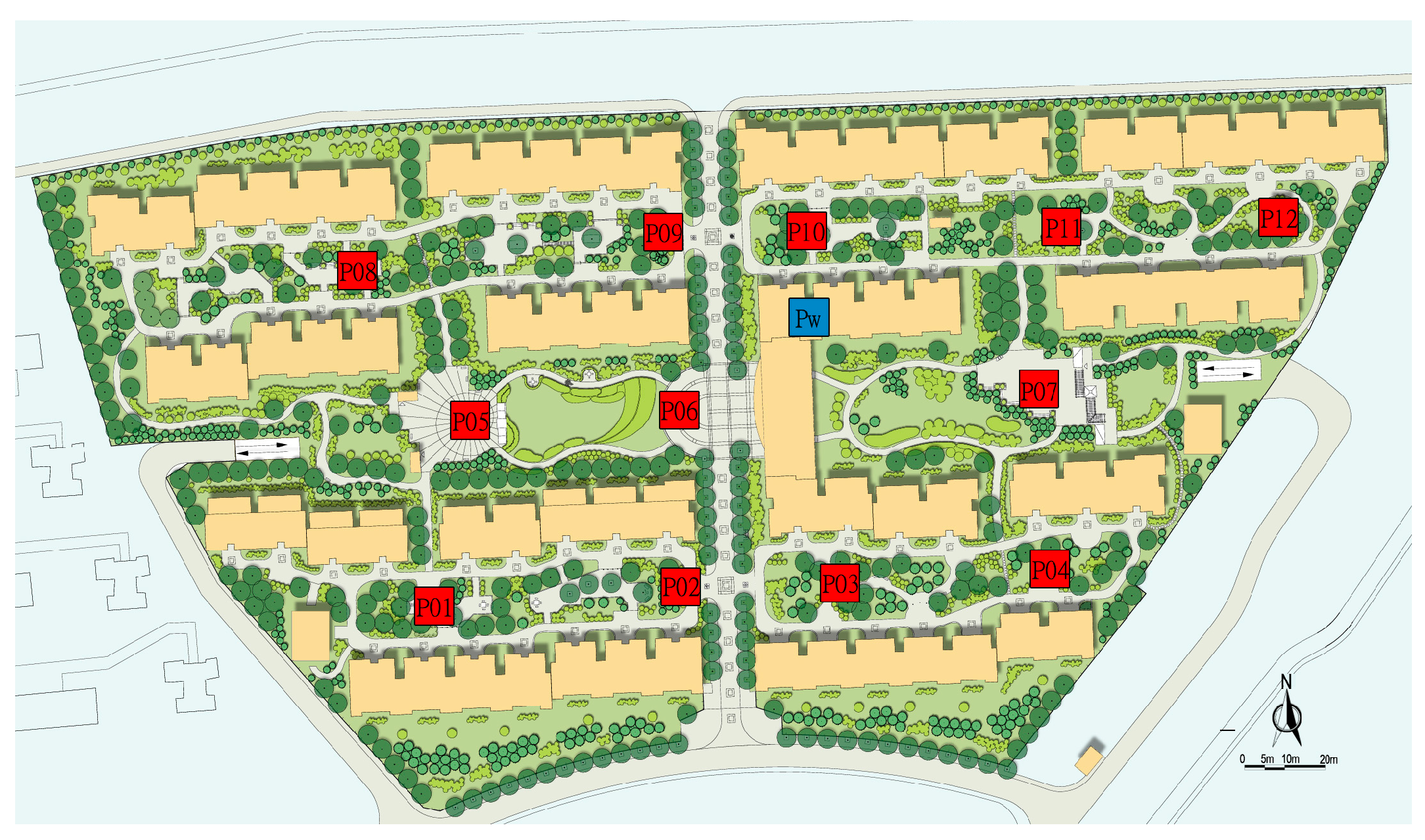
Figure 2.
On-site measurements of (a) average wind velocity and wind direction by hour and (b) average PM2.5 by hour of Pw.
Figure 2.
On-site measurements of (a) average wind velocity and wind direction by hour and (b) average PM2.5 by hour of Pw.

Figure 3.
Model validation: comparison of the simulation results and measurement data for wind velocity (a) and PM2.5 (b).
Figure 3.
Model validation: comparison of the simulation results and measurement data for wind velocity (a) and PM2.5 (b).

Figure 4.
Case setting (27 cases were set by combining tree crown morphologies with three levels of LADs and aspect ratios).
Figure 4.
Case setting (27 cases were set by combining tree crown morphologies with three levels of LADs and aspect ratios).
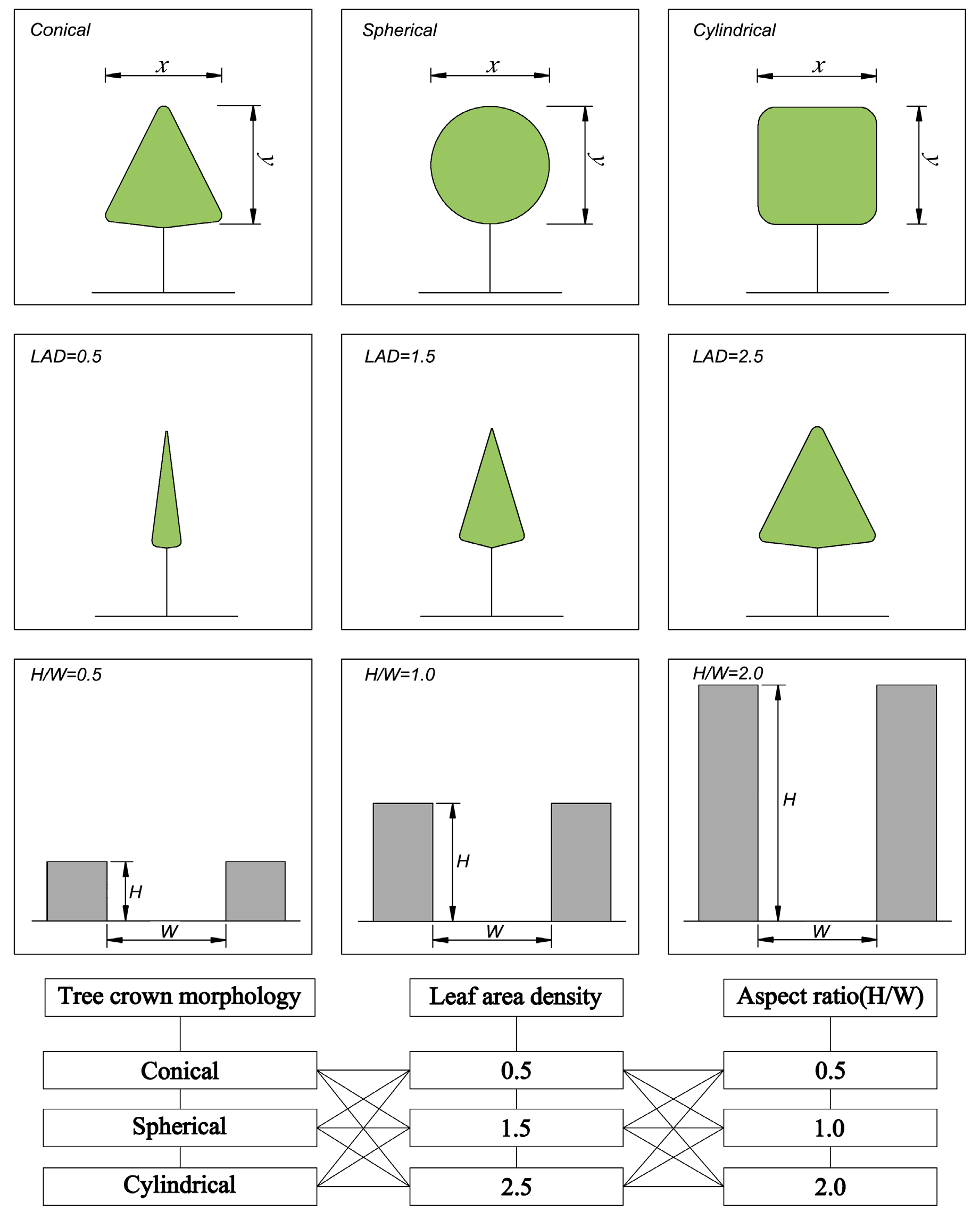
Figure 5.
The computational domain.

Figure 6.
Air velocity and streamline fields at z = 1.5 m in H/W = 0.5 (left), H/W = 1.0 (middle), and H/W = 2.0 (right) for tree-free scenarios (a–c), LAD = 0.5 (d–f), LAD = 1.5 (g–i), and LAD = 2.5 (j–l) with conical canopy.
Figure 6.
Air velocity and streamline fields at z = 1.5 m in H/W = 0.5 (left), H/W = 1.0 (middle), and H/W = 2.0 (right) for tree-free scenarios (a–c), LAD = 0.5 (d–f), LAD = 1.5 (g–i), and LAD = 2.5 (j–l) with conical canopy.

Figure 7.
Air velocity and streamline fields at y = 380 m in H/W = 0.5 (left), H/W = 1.0 (middle), and H/W = 2.0 (right) for tree-free scenarios (a–c), LAD = 0.5 (d–f), LAD = 1.5 (g–i), and LAD = 2.5 (j–l) with conical canopy.
Figure 7.
Air velocity and streamline fields at y = 380 m in H/W = 0.5 (left), H/W = 1.0 (middle), and H/W = 2.0 (right) for tree-free scenarios (a–c), LAD = 0.5 (d–f), LAD = 1.5 (g–i), and LAD = 2.5 (j–l) with conical canopy.
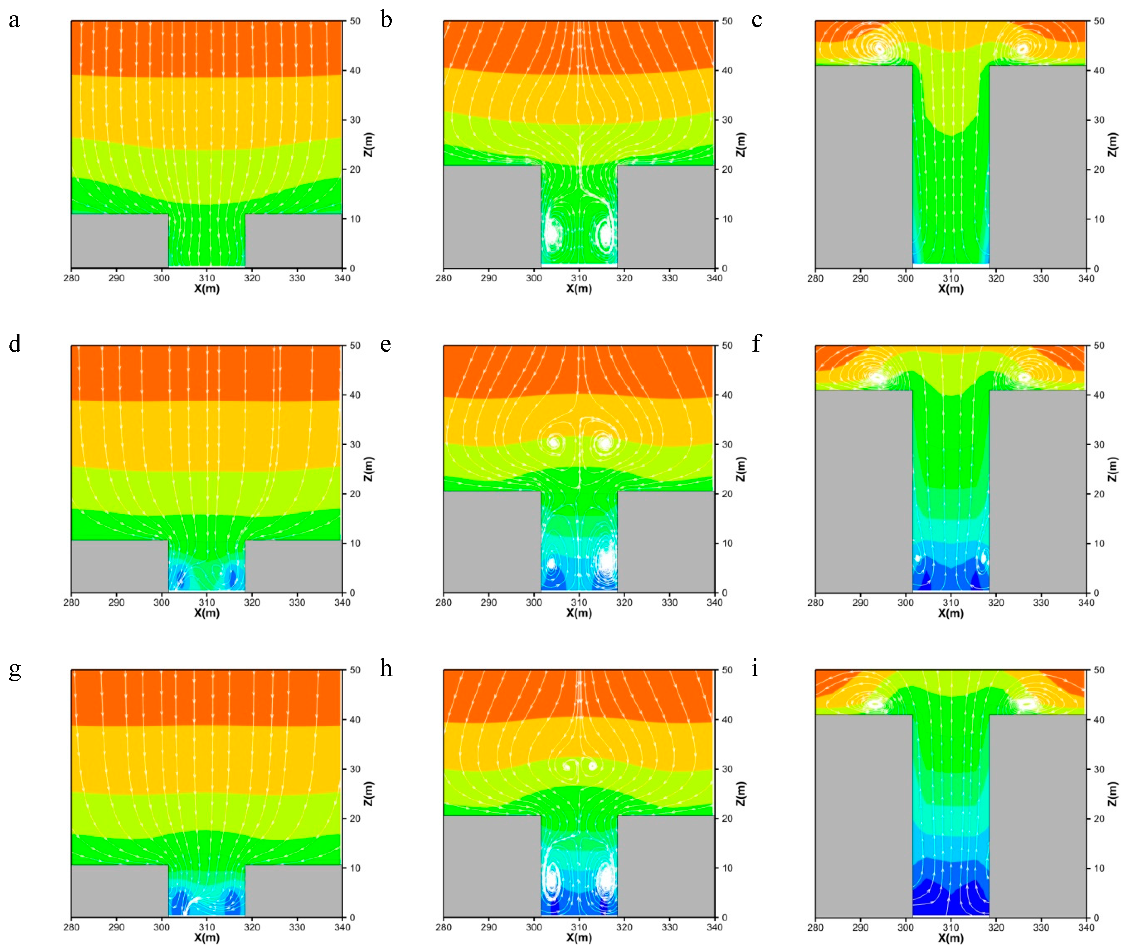

Figure 8.
Average air velocity at z = 1.5 m for the conical (a), spherical (b), and cylindrical (c) canopies.
Figure 8.
Average air velocity at z = 1.5 m for the conical (a), spherical (b), and cylindrical (c) canopies.
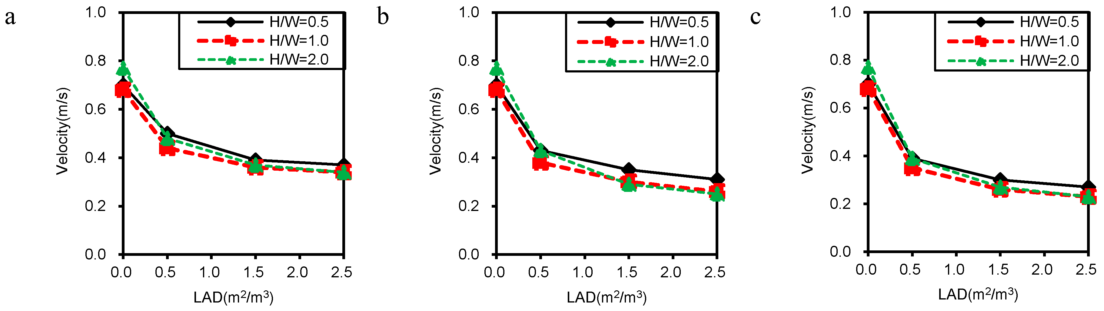
Figure 9.
PM2.5 distributions at z = 1.5 m in H/W = 0.5 (left), H/W = 1.0 (middle), and H/W = 2.0 (right) for tree-free scenarios (a–c), LAD = 0.5 (d–f), LAD = 1.5 (g–i), and LAD = 2.5 (j–l) with conical canopy.
Figure 9.
PM2.5 distributions at z = 1.5 m in H/W = 0.5 (left), H/W = 1.0 (middle), and H/W = 2.0 (right) for tree-free scenarios (a–c), LAD = 0.5 (d–f), LAD = 1.5 (g–i), and LAD = 2.5 (j–l) with conical canopy.

Figure 10.
Reduction ratio at z = 1.5 m in average PM2.5 for conical (a), spherical (b), and cylindrical (c) canopies.
Figure 10.
Reduction ratio at z = 1.5 m in average PM2.5 for conical (a), spherical (b), and cylindrical (c) canopies.

Figure 11.
Reduction ratio at z = 1.5 m in average PM2.5 for H/W = 0.5 (a), H/W = 1.0 (b), and H/W = 2.0 (c).
Figure 11.
Reduction ratio at z = 1.5 m in average PM2.5 for H/W = 0.5 (a), H/W = 1.0 (b), and H/W = 2.0 (c).

Figure 12.
PM2.5 for H/W = 0.5 (left), H/W = 1.0 (middle), H/W = 2.0 (right) for the conical (a–c), spherical (d–f), and cylindrical (g–i) canopies along the vertical line located at x = 320 m and y = 310 m (Line A from Figure 5).
Figure 12.
PM2.5 for H/W = 0.5 (left), H/W = 1.0 (middle), H/W = 2.0 (right) for the conical (a–c), spherical (d–f), and cylindrical (g–i) canopies along the vertical line located at x = 320 m and y = 310 m (Line A from Figure 5).


Table 1.
Vegetation parameter setting in numerical simulations.
| Typical Plants | 3D Geometric Figure | Crown Volume Expressions | CH(y) (m) | CD(x) (m) | CBH (m) | LAD (m2/m3) | Vd (m/s) [9,10] |
|---|---|---|---|---|---|---|---|
| Picea wilsonii | Cone | πx2y/12 | 5 | 3 | 0.5 | 1.71 | 0.0252 |
| Pinus tabulaeformis | Cone | πx2y/12 | 6 | 3 | 1 | 1.69 | 0.0175 |
| Platycladus orientalis | Cone | πx2y/12 | 6 | 5 | 0.5 | 2.20 | 0.0407 |
| Ginkgo biloba | Cone | πx2y/12 | 7 | 3 | 2 | 1.26 | 0.0245 |
| Koelreuteria paniculata | Oval | πx2y/6 | 8.5 | 4 | 2.5 | 1.54 | 0.0081 |
| Acer truncatum | Oval | πx2y/6 | 6.5 | 4 | 1.5 | 0.92 | 0.0122 |
| Sabina chinensis | Cone | πx2y/12 | 3.5 | 3 | 0.5 | 0.83 | 0.0068 |
| Syringa oblata | Sphericity | πx2y/6 | 1 | 1.5 | 0 | 0.96 | 0.0075 |
Table 2.
Paired sample t-test for the validation criteria comparing the on-site measured and simulation results.
Table 2.
Paired sample t-test for the validation criteria comparing the on-site measured and simulation results.
| Comparison Criteria | Paired Differences | t | Significance Value (Two-Tailed) 1 | ||||
|---|---|---|---|---|---|---|---|
| Mean | Standard Deviation | Standard Error Mean | 95% Confidence Interval of the Difference | ||||
| Lower | Upper | ||||||
| PM2.5 | 1.80 | 15.63 | 3.19 | −4.80 | 8.40 | 0.56 | 0.578 |
| Air velocity | 0.0054 | 0.1331 | 0.0272 | −0.0508 | 0.0616 | 0.20 | 0.844 |
1 Significant at 0.05 level.
Table 3.
Tree configuration setting.
| Tree Crown Morphology | Typical Avenue Trees | Crown Volume Expression 1 | Vd |
|---|---|---|---|
| Conical | Fraxinus pennsylvanica × F. velutina | πx2y/12 | 0.0036 |
| Spherical | Sophora japonica | πx2y/6 | 0.0068 |
| Cylindrical | Populus tomentosa | πx2y/4 | 0.0075 |
1 x is the crown diameter (m), y is the crown height (m), and Vd is the deposition velocity on tree leaves (m/s).
© 2017 by the authors. Licensee MDPI, Basel, Switzerland. This article is an open access article distributed under the terms and conditions of the Creative Commons Attribution (CC BY) license (http://creativecommons.org/licenses/by/4.0/).
Share and Cite
MDPI and ACS Style
Hong, B.; Lin, B.; Qin, H. Numerical Investigation on the Effect of Avenue Trees on PM2.5 Dispersion in Urban Street Canyons. Atmosphere 2017, 8, 129. https://doi.org/10.3390/atmos8070129
AMA Style
Hong B, Lin B, Qin H. Numerical Investigation on the Effect of Avenue Trees on PM2.5 Dispersion in Urban Street Canyons. Atmosphere. 2017; 8(7):129. https://doi.org/10.3390/atmos8070129
Chicago/Turabian StyleHong, Bo, Borong Lin, and Hongqiao Qin. 2017. "Numerical Investigation on the Effect of Avenue Trees on PM2.5 Dispersion in Urban Street Canyons" Atmosphere 8, no. 7: 129. https://doi.org/10.3390/atmos8070129
Note that from the first issue of 2016, this journal uses article numbers instead of page numbers. See further details here.