Overview of Model Inter-Comparison in Japan’s Study for Reference Air Quality Modeling (J-STREAM)

 , , ,
, , ,
Abstract
:1. Introduction
2. History of Model Inter-Comparison Related to Japan
3. Objective of J-STREAM
4. Methodology
4.1. Target Periods
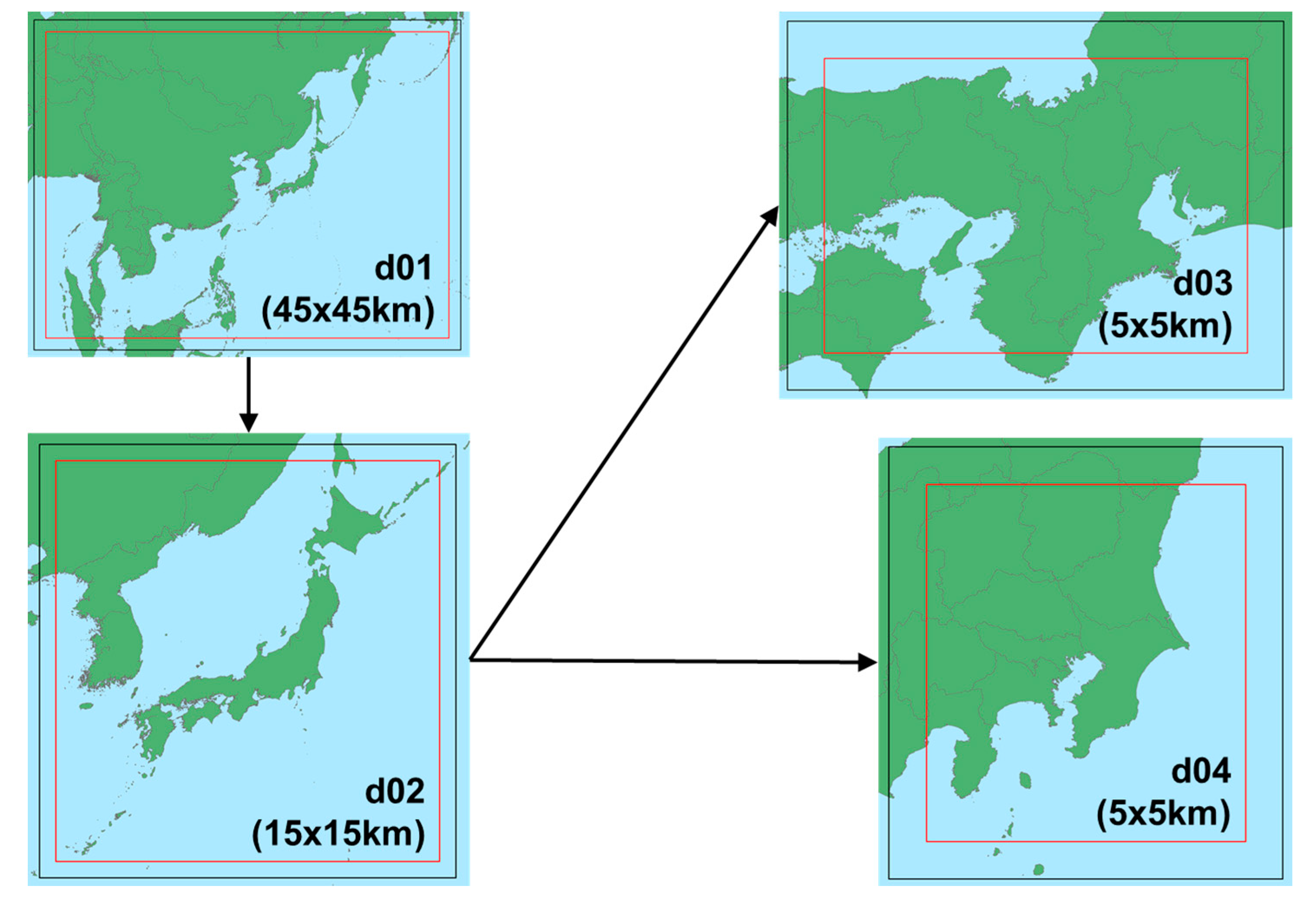
4.2. Target Domains
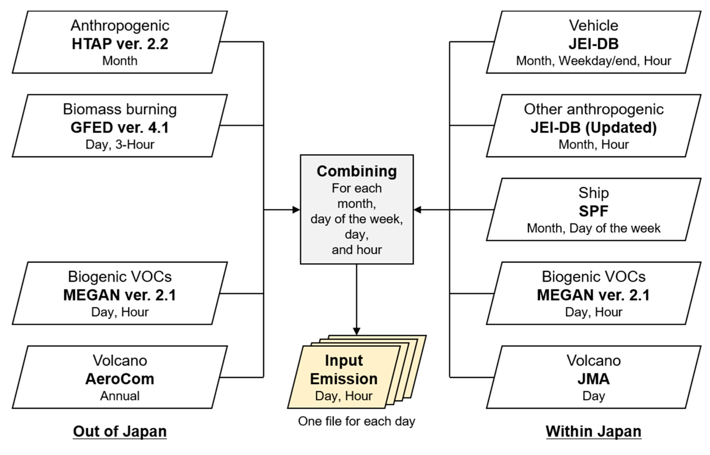
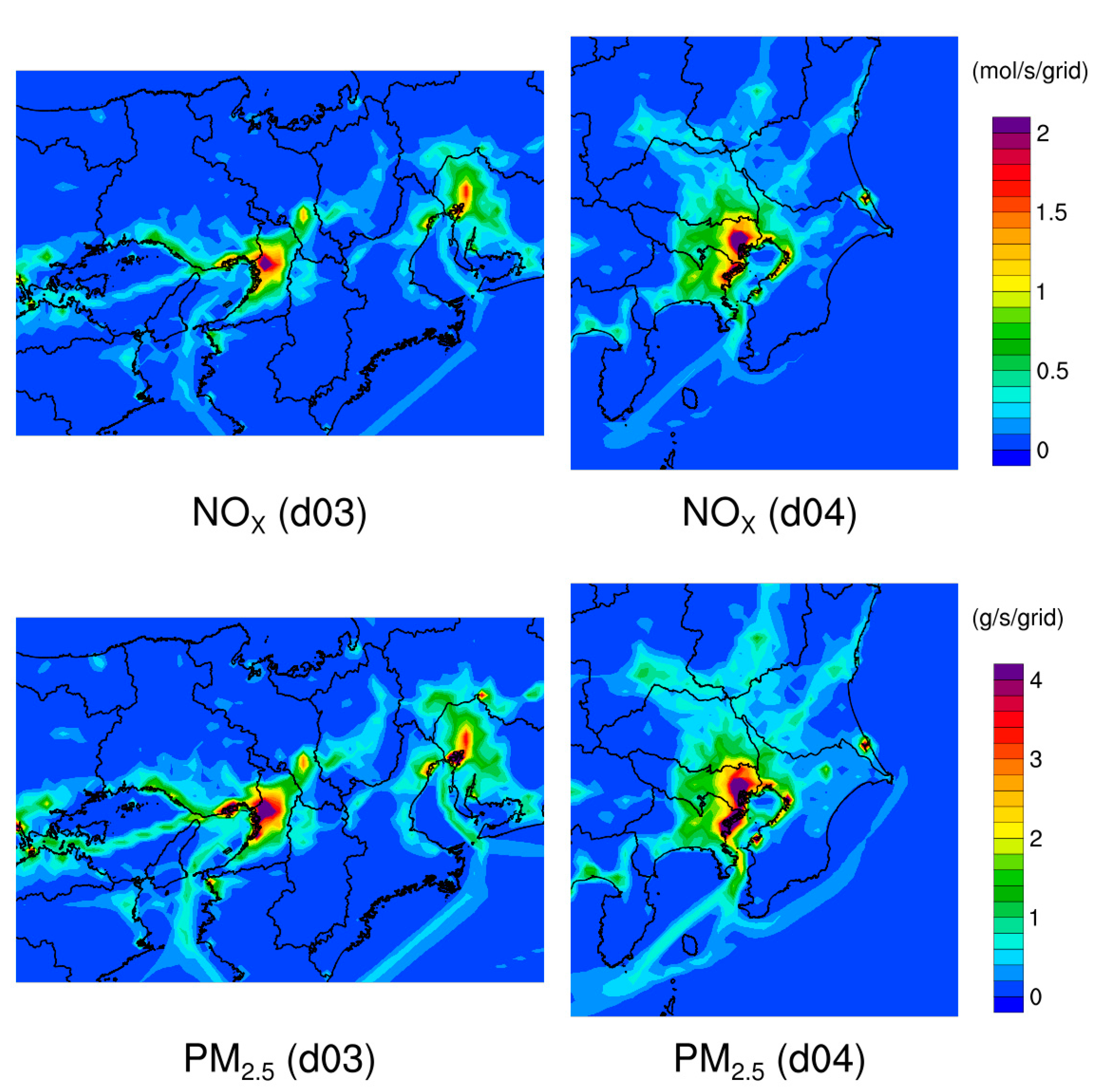
4.3. Emission Inputs
4.4. Meteorology Inputs
4.5. Initial and Boundary Concentrations
4.6. Observation Data
4.7. Data Treatment
5. Status
6. Future Direction
Acknowledgments
Author Contributions
Conflicts of Interest
References
- Wakamatsu, S.; Morikawa, T.; Ito, A. Air pollution trends in Japan between 1970 and 2012 and impact of urban air pollution countermeasures. Asian J. Atmos. Environ. 2013, 7, 177–190. [Google Scholar] [CrossRef]
- Meng, Z.; Dabdub, D.; Seinfeld, J.H. Chemical coupling between atmospheric ozone and particulate matter. Science 1997, 277, 116–119. [Google Scholar] [CrossRef]
- Carmichael, G.R.; Calori, G.; Hayami, H.; Uno, I.; Cho, S.Y.; Engardt, M.; Kim, S.B.; Ichikawa, Y.; Ikeda, Y.; Woo, J.H.; et al. The MICS-Asia study: Model intercomparison of long-range transport and sulfur deposition in East Asia. Atmos. Environ. 2002, 36, 175–199. [Google Scholar] [CrossRef]
- Carmichael, G.R.; Sakurai, T.; Streets, D.; Hozumi, Y.; Ueda, H.; Park, S.U.; Fung, C.; Han, Z.; Kajino, M.; Engardt, M.; et al. MICS-Asia II: The model intercomparison study for Asia phase II methodology and overview of findings. Atmos. Environ. 2008, 42, 3468–3490. [Google Scholar] [CrossRef]
- Galmarini, S.; Koffi, B.; Solazzo, E.; Keating, T.; Hogrefe, C.; Schulz, M.; Benedictow, A.; Griesfeller, J.J.; Janssens-Maenhout, G.; Carmichael, G.; et al. Technical note: Coordination and harmonization of the multi-scale, multi-model activities HTAP2, AQMEII3, and MICS-Asia3: Simulations, emission inventories, boundary conditions, and model output formats. Atmos. Chem. Phys. 2017, 17, 1543–1555. [Google Scholar] [CrossRef]
- Morino, Y.; Chatani, S.; Hayami, H.; Sasaki, K.; Mori, Y.; Morikawa, T.; Ohara, T.; Hasegawa, S.; Kobayashi, S. Inter-comparison of chemical transport models and evaluation of model performance for O3 and PM2.5 prediction—Case study in the Kanto area in summer 2007. J. Jpn. Soc. Atmos. Environ. 2010, 45, 212–226. [Google Scholar]
- Chatani, S.; Morino, Y.; Shimadera, H.; Hayami, H.; Mori, Y.; Sasaki, K.; Kajino, M.; Yokoi, T.; Morikawa, T.; Ohara, T. Multi-model analyses of dominant factors influencing elemental carbon in Tokyo metropolitan area of Japan. Aerosol Air Qual. Res. 2014, 14, 396–405. [Google Scholar] [CrossRef]
- Shimadera, H.; Hayami, H.; Chatani, S.; Morino, Y.; Mori, Y.; Morikawa, T.; Yamaji, K.; Ohara, T. Sensitivity analyses of factors influencing CMAQ performance for fine particulate nitrate. J. Air Waste Manag. Assoc. 2014, 64, 374–387. [Google Scholar] [CrossRef] [PubMed]
- Morino, Y.; Chatani, S.; Hayami, H.; Sasaki, K.; Mori, Y.; Morikawa, T.; Ohara, T.; Hasegawa, S.; Kobayashi, S. Evaluation of ensemble approach for O3 and PM2.5 simulation. Asian J. Atmos. Environ. 2010, 4, 150–156. [Google Scholar] [CrossRef]
- Byun, D.; Schere, K.L. Review of the governing equations, computational algorithms, and other components of the models-3 community multiscale air quality (CMAQ) modeling system. Appl. Mech. Rev. 2006, 59, 51–77. [Google Scholar] [CrossRef]
- Shimadera, H.; Hayami, H.; Morino, Y.; Ohara, T.; Chatani, S.; Hasegawa, S.; Kaneyasu, N. Analysis of summertime atmospheric transport of fine particulate matter in Northeast Asia. Asia-Pac. J. Atmos. Sci. 2013, 49, 347–360. [Google Scholar] [CrossRef]
- Kajino, M.; Inomata, Y.; Sato, K.; Ueda, H.; Han, Z.; An, J.; Katata, G.; Deushi, M.; Maki, T.; Oshima, N.; et al. Development of the RAQM2 aerosol chemical transport model and predictions of the northeast asian aerosol mass, size, chemistry, and mixing type. Atmos. Chem. Phys. 2012, 12, 11833–11856. [Google Scholar] [CrossRef] [Green Version]
- Shimadera, H.; Hayami, H.; Chatani, S.; Morikawa, T.; Morino, Y.; Mori, Y.; Yamaji, K.; Nakatsuka, S.; Ohara, T. Urban air quality model inter-comparison study in Japan (UMICS) for improvement of PM2.5 simulation. Asian J. Atmos. Environ. 2017, in press. [Google Scholar]
- Shimadera, H.; Hayami, H.; Chatani, S.; Morikawa, T.; Morino, Y.; Ohara, T.; Mori, Y.; Yamaji, K.; Nakatsuka, S. Comprehensive Sensitivity Analyses on Air Quality Model Performance for PM2.5 Simulation. In Proceedings of the 16th International Conference on Harmonisation within Atmospheric Dispersion Modelling for Regulatory Purposes, Varna, Bulgaria, 8–11 September 2014. [Google Scholar]
- Morino, Y.; Nagashima, T.; Sugata, S.; Sato, K.; Tanabe, K.; Noguchi, T.; Takami, A.; Tanimoto, H.; Ohara, T. Verification of chemical transport models for PM2.5 chemical composition using simultaneous measurement data over Japan. Aerosol Air Qual. Res. 2015, 15, 2009–2023. [Google Scholar] [CrossRef]
- Robinson, A.L.; Donahue, N.M.; Shrivastava, M.K.; Weitkamp, E.A.; Sage, A.M.; Grieshop, A.P.; Lane, T.E.; Pierce, J.R.; Pandis, S.N. Rethinking organic aerosols: Semivolatile emissions and photochemical aging. Science 2007, 315, 1259–1262. [Google Scholar] [CrossRef] [PubMed]
- Itahashi, S.; Uno, I.; Osada, K.; Kamiguchi, Y.; Yamamoto, S.; Tamura, K.; Wang, Z.; Kurosaki, Y.; Kanaya, Y. Nitrate transboundary heavy pollution over East Asia in winter. Atmos. Chem. Phys. 2017, 17, 3823–3843. [Google Scholar] [CrossRef]
- Yoshikado, H. Summertime behavior of the precursors (non-methane hydrocarbons and nitrogen oxides) related with high concentrations of ozone in the Tokyo metropolitan area. J. Jpn. Soc. Atmos. Environ. 2015, 50, 44–51. [Google Scholar]
- Kiriyama, Y.; Shimadera, H.; Itahashi, S.; Hayami, H.; Miura, K. Evaluation of the effect of regional pollutants and residual ozone on ozone concentrations in the morning in the inland of the kanto region. Asian J. Atmos. Environ. 2015, 9, 1–11. [Google Scholar] [CrossRef]
- Sun, Y.L.; Jiang, Q.; Wang, Z.F.; Fu, P.Q.; Li, J.; Yang, T.; Yin, Y. Investigation of the sources and evolution processes of severe haze pollution in Beijing in January 2013. J. Geophys. Res. Atmos. 2014, 119, 4380–4398. [Google Scholar] [CrossRef]
- Uno, I.; Sugimoto, N.; Shimizu, A.; Yumimoto, K.; Hara, Y.; Wang, Z.F. Record heavy PM2.5 air pollution over China in January 2013: Vertical and horizontal dimensions. Sola 2014, 10, 136–140. [Google Scholar] [CrossRef]
- Zheng, G.J.; Duan, F.K.; Su, H.; Ma, Y.L.; Cheng, Y.; Zheng, B.; Zhang, Q.; Huang, T.; Kimoto, T.; Chang, D.; et al. Exploring the severe winter haze in Beijing: The impact of synoptic weather, regional transport and heterogeneous reactions. Atmos. Chem. Phys. 2015, 15, 2969–2983. [Google Scholar] [CrossRef]
- Janssens-Maenhout, G.; Crippa, M.; Guizzardi, D.; Dentener, F.; Muntean, M.; Pouliot, G.; Keating, T.; Zhang, Q.; Kurokawa, J.; Wankmuller, R.; et al. HTAP_v2.2: A mosaic of regional and global emission grid maps for 2008 and 2010 to study hemispheric transport of air pollution. Atmos. Chem. Phys. 2015, 15, 11411–11432. [Google Scholar] [CrossRef] [Green Version]
- Van der Werf, G.R.; Randerson, J.T.; Giglio, L.; van Leeuwen, T.T.; Chen, Y.; Rogers, B.M.; Mu, M.; van Marle, M.J.E.; Morton, D.C.; Collatz, G.J.; et al. Global fire emissions estimates during 1997–2016. Earth Syst. Sci. Data 2017, 9, 697–720. [Google Scholar] [CrossRef]
- Guenther, A.B.; Jiang, X.; Heald, C.L.; Sakulyanontvittaya, T.; Duhl, T.; Emmons, L.K.; Wang, X. The model of emissions of gases and aerosols from nature version 2.1 (megan2.1): An extended and updated framework for modeling biogenic emissions. Geosci. Model Dev. 2012, 5, 1471–1492. [Google Scholar] [CrossRef] [Green Version]
- Diehl, T.; Heil, A.; Chin, M.; Pan, X.; Streets, D.; Schultz, M.; Kinne, S. Anthropogenic, biomass burning, and volcanic emissions of black carbon, organic carbon, and SO2 from 1980 to 2010 for hindcast model experiments. Atmos. Chem. Phys. 2012, 2012, 24895–24954. [Google Scholar] [CrossRef] [Green Version]
- Chatani, S.; Morikawa, T.; Nakatsuka, S.; Matsunaga, S.; Minoura, H. Development of a framework for a high-resolution, three-dimensional regional air quality simulation and its application to predicting future air quality over Japan. Atmos. Environ. 2011, 45, 1383–1393. [Google Scholar] [CrossRef]
- Japan Meteorological Agency. Available online: http://www.data.jma.go.jp/svd/vois/data/tokyo/volcano.html (accessed on 27 October 2017).
- Carter, W.P.L. Development of the SAPRC-07 chemical mechanism. Atmos. Environ. 2010, 44, 5324–5335. [Google Scholar] [CrossRef]
- Carter, W.P.L. Documentation of the SAPRC-99 Chemical Mechanism for Voc Reactivity Assessment; California Environmental Protection Agency: Sacramento, CA, USA, 2000.
- Whitten, G.Z.; Heo, G.; Kimura, Y.; McDonald-Buller, E.; Allen, D.T.; Carter, W.P.L.; Yarwood, G. A new condensed toluene mechanism for carbon bond CB05-TU. Atmos. Environ. 2010, 44, 5346–5355. [Google Scholar] [CrossRef]
- Goliff, W.S.; Stockwell, W.R.; Lawson, C.V. The regional atmospheric chemistry mechanism, version 2. Atmos. Environ. 2013, 68, 174–185. [Google Scholar] [CrossRef]
- Stockwell, W.R.; Middleton, P.; Chang, J.S.; Tang, X. The second generation regional acid deposition model chemical mechanism for regional air quality modeling. J. Geophys. Res. Atmos. 1990, 95, 16343–16367. [Google Scholar] [CrossRef]
- Uranishi, K.; Ikemori, F.; Nakatsubo, R.; Shimadera, H.; Kondo, A.; Kikutani, Y.; Asano, K.; Sugata, S. Identification of biased sectors in emission data using a combination of chemical transport model and receptor model. Atmos. Environ. 2017, 166, 166–181. [Google Scholar] [CrossRef]
- Skamarock, W.C.; Klemp, J.B.; Dudhia, J.; Gill, D.O.; Barker, D.M.; Duda, M.G.; Huang, X.Y.; Wang, W.; Power, J.G. A Description of the Advanced Research WRF Version 3; NCAR/TN-475+STR; National Center for Atmospheric Research: Boulder, CO, USA, 2008. [Google Scholar]
- National Centers for Environmental Prediction/National Weather Service/NOAA/U.S. Department of Commerce. NCEP FNL Operational Model Global Tropospheric Analyses, Continuing from July 1999; Research Data Archive at the National Center for Atmospheric Research, Computational and Information Systems Laboratory: Boulder, CO, USA, 2000.
- Gemmill, W.; Katz, B.; Li, X. The Daily Real-Time, Global Sea Surface Temperature—High Resolution Analysis: RTG_SST_HR; Environmental Modeling Center: Camp Springs, MD, USA, 2007. [Google Scholar]
- Hong, S.Y.; Dudhia, J.; Chen, S.H. A revised approach to ice microphysical processes for the bulk parameterization of clouds and precipitation. Mon. Weather Rev. 2004, 132, 103–120. [Google Scholar] [CrossRef]
- Mlawer, E.J.; Taubman, S.J.; Brown, P.D.; Iacono, M.J.; Clough, S.A. Radiative transfer for inhomogeneous atmospheres: RRTM, a validated correlated-k model for the longwave. J. Geophys. Res. Atmos. 1997, 102, 16663–16682. [Google Scholar] [CrossRef]
- Dudhia, J. Numerical study of convection observed during the winter monsoon experiment using a mesoscale two-dimensional model. J. Atmos. Sci. 1989, 46, 3077–3107. [Google Scholar] [CrossRef]
- Nakanishi, M.; Niino, H. An improved mellor–yamada level-3 model: Its numerical stability and application to a regional prediction of advection fog. Bound.-Layer Meteorol. 2006, 119, 397–407. [Google Scholar] [CrossRef]
- Chen, F.; Dudhia, J. Coupling an advanced land surface-hydrology model with the penn state-NCAR MM5 modeling system. Part I: Model implementation and sensitivity. Mon. Weather Rev. 2001, 129, 569–585. [Google Scholar] [CrossRef]
- Kain, J.S. The kain-fritsch convective parameterization: An update. J. Appl. Meteorol. 2004, 43, 170–181. [Google Scholar] [CrossRef]
- Kusaka, H.; Kondo, H.; Kikegawa, Y.; Kimura, F. A simple single-layer urban canopy model for atmospheric models: Comparison with multi-layer and slab models. Bound.-Layer Meteorol. 2001, 101, 329–358. [Google Scholar] [CrossRef]
- Sudo, K.; Takahashi, M.; Kurokawa, J.; Akimoto, H. Chaser: A global chemical model of the troposphere—1. Model description. J. Geophys. Res. Atmos. 2002, 107. [Google Scholar] [CrossRef]
- Huang, M.; Carmichael, G.R.; Pierce, R.B.; Jo, D.S.; Park, R.J.; Flemming, J.; Emmons, L.K.; Bowman, K.W.; Henze, D.K.; Davila, Y.; et al. Impact of intercontinental pollution transport on north american ozone air pollution: An HTAP phase 2 multi-model study. Atmos. Chem. Phys. 2017, 17, 5721–5750. [Google Scholar] [CrossRef]
- Emmons, L.K.; Walters, S.; Hess, P.G.; Lamarque, J.F.; Pfister, G.G.; Fillmore, D.; Granier, C.; Guenther, A.; Kinnison, D.; Laepple, T.; et al. Description and evaluation of the model for ozone and related chemical tracers, version 4 (MOZART-4). Geosci. Model Dev. 2010, 3, 43–67. [Google Scholar] [CrossRef] [Green Version]
- National Institute for Environmental Studies. Available online: https://www.nies.go.jp/igreen/ (accessed on 29 August 2017).
- Ministry of the Environment. Available online: http://www.env.go.jp/air/osen/pm/monitoring.html (accessed on 29 August 2017).
- Ministry of the Environment. Available online: http://www.env.go.jp/air/osen/jokyo_h25/rep08_h25.pdf (accessed on 28 September 2017).
- Grell, G.A.; Peckham, S.E.; Schmitz, R.; McKeen, S.A.; Frost, G.; Skamarock, W.C.; Eder, B. Fully coupled “online” chemistry within the WRF model. Atmos. Environ. 2005, 39, 6957–6975. [Google Scholar] [CrossRef]
- Dunker, A.M.; Yarwood, G.; Ortmann, J.P.; Wilson, G.M. Comparison of source apportionment and source sensitivity of ozone in a three-dimensional air quality model. Environ. Sci. Technol. 2002, 36, 2953–2964. [Google Scholar] [CrossRef] [PubMed]
- Wagstrom, K.M.; Pandis, S.N.; Yarwood, G.; Wilson, G.M.; Morris, R.E. Development and application of a computationally efficient particulate matter apportionment algorithm in a three-dimensional chemical transport model. Atmos. Environ. 2008, 42, 5650–5659. [Google Scholar] [CrossRef]
- Yang, Y.J.; Wilkinson, J.G.; Russell, A.G. Fast, direct sensitivity analysis of multidimensional photochemical models. Environ. Sci. Technol. 1997, 31, 2859–2868. [Google Scholar] [CrossRef]
- Chatani, S.; Morikawa, T.; Nakatsuka, S.; Matsunaga, S. Sensitivity analyses of domestic emission sources and transboundary transport on PM2.5 concentrations in three major Japanese urban areas for the year 2005 with the three-dimensional air quality simulation. J. Jpn. Soc. Atmos. Environ. 2011, 46, 101–110. [Google Scholar]
- Ikeda, K.; Yamaji, K.; Kanaya, Y.; Taketani, F.; Pan, X.; Komazaki, Y.; Kurokawa, J.-I.; Ohara, T. Source region attribution of PM2.5 mass concentrations over Japan. Geochem. J. 2015, 49, 185–194. [Google Scholar] [CrossRef]
- Itahashi, S.; Hayami, H.; Uno, I. Comprehensive study of emission source contributions for tropospheric ozone formation over East Asia. J. Geophys. Res. Atmos. 2015, 120, 331–358. [Google Scholar] [CrossRef]
- Itahashi, S.; Hayami, H.; Yumimoto, K.; Uno, I. Chinese province-scale source apportionments for sulfate aerosol in 2005 evaluated by the tagged tracer method. Environ. Pollut. 2017, 220, 1366–1375. [Google Scholar] [CrossRef] [PubMed]
- Nagashima, T.; Sudo, K.; Akimoto, H.; Kurokawa, J.; Ohara, T. Long-term change in the source contribution to surface ozone over Japan. Atmos. Chem. Phys. 2017, 17, 8231–8246. [Google Scholar] [CrossRef]
- Yamaji, K.; Uno, I.; Irie, H. Investigating the response of east asian ozone to chinese emission changes using a linear approach. Atmos. Environ. 2012, 55, 475–482. [Google Scholar] [CrossRef]
- Takahashi, K.; Fushimi, A.; Morino, Y.; Iijima, A.; Yonemochi, S.-I.; Hayami, H.; Hasegawa, S.; Tanabe, K.; Kobayash, S. Source apportionment of ambient fine particle using a receptor model combined with radiocarbon content in Northern Kanto area. J. Jpn. Soc. Atmos. Environ. 2011, 46, 156–163. [Google Scholar]
- Cohan, D.S.; Napelenok, S.L. Air quality response modeling for decision support. Atmosphere 2011, 2, 407–425. [Google Scholar] [CrossRef]


| Region | Project | Domain | Emission | Meteorology | Duration | Reference |
|---|---|---|---|---|---|---|
| Asia | MICS-Asia1 | Fixed | Provided | Provided | 1998–2002 | [3] |
| MICS-Asia2 | Own | Provided | Own | 2003–2009 | [4] | |
| MICS-Asia3 | Fixed | Provided | Provided | 2010-ongoing | [5] | |
| Japan | FAMIKA | Own | Own | Own | 2008–2009 | [6] |
| UMICS | Fixed | Provided | Provided | 2010–2012 | [7,8] | |
| J-STREAM | Fixed | Provided | Provided | 2016–2018 |
| Dates | |
|---|---|
| Winter 2013 | 11 January 2013 to 9 February 2013 |
| Spring 2013 | 27 April 2013 to 26 May 2013 |
| Summer 2013 | 12 July 2013 to 10 August 2013 |
| Autumn 2013 | 11 October 2013 to 9 November 2013 |
| Winter 2014 | 10 January 2014 to 8 February 2014 |
| Options | Schemes and Settings Used |
|---|---|
| Microphysics | WRF Single-Moment 5-class scheme [38] |
| Longwave radiation | RRTM scheme [39] |
| Shortwave radiation | Dudhia scheme [40] |
| Surface layer | Mellor-Yamada Nakanishi and Niino surface layer scheme [41] |
| Land surface | Noah Land Surface Model [42] |
| Planetary boundary layer | Mellor-Yamada Nakanishi and Niino Level 3 PBL scheme [41] |
| Cumulus parameterization | Kain-Fritsch scheme [43] (Only in d01 and d02) |
| Grid nudging (Wind, temperature, and water vapour) | 1.0 × 10⁻⁴ (in d01) 0.5 × 10⁻⁵ (in d02) 0 (in d03 and d04) |
| No. | Model | Version | Chemical Mechanism | Aerosol Module | Emission | Meteorology | Boundary (d01) | Domains | |||
|---|---|---|---|---|---|---|---|---|---|---|---|
| d01 | d02 | d03 | d04 | ||||||||
| 1 | CMAQ | 5.1 | SAPRC07 | aero6 | Provided | Provided | x | x | |||
| 2 | CMAQ | 5.1 | SAPRC07 | aero6 | Provided | Provided | x | x | |||
| 3 | CMAQ | 5.1 | SAPRC07 | aero6 | Provided | Provided | x | x | |||
| 4 | CMAQ | 5.1 | SAPRC07 | aero6 | Provided | Provided | Provided | x | x | x | x |
| 5 | CMAQ | 5.1 | SAPRC07 | aero6 | Own | Provided | Provided | x | x | x | x |
| 6 | CMAQ | 5.0.2 | SAPRC99 | aero5 | Provided | Provided | x | x | |||
| 7 | CMAQ | 5.0.2 | SAPRC99 | aero5 | Provided | Provided | Provided | x | x | x | x |
| 8 | CMAQ | 5.0.2 | SAPRC07 | aero6 | Provided | Provided | Provided | x | x | x | x |
| 9 | CMAQ | 5.0.2 | SAPRC07 | aero6 | Provided | Own | MOZART | x | x | x | x |
| 10 | CMAQ | 5.0.2 | SAPRC07 | aero6 | Provided | Provided | x | x | |||
| 11 | CMAQ | 5.0.2 | SAPRC07 | aero6 | Provided | Provided | Provided | x | x | x | x |
| 12 | CMAQ | 5.0.2 | RACM2 | aero6 | Provided | Provided | x | x | |||
| 13 | CMAQ | 5.0.2 | RACM2 | aero6 | Provided | Provided | Provided | x | x | x | x |
| 14 | CMAQ | 5.0.2 | CB05 | aero6 | Provided | Provided | x | x | |||
| 15 | CMAQ | 5.0.2 | CB05 | aero6 | Provided | Provided | Provided | x | x | x | x |
| 16 | CMAQ | 5.0.2 | CB05 | aero6 | Provided | Provided | Provided | x | x | x | x |
| 17 | CMAQ | 5.0.2 | CB05 | aero6vbs | Provided | Provided | Provided | x | x | x | x |
| 18 | CMAQ | 5.0.1 | SAPRC99 | aero5 | Provided | Provided | x | ||||
| 19 | CMAQ | 5.0.1 | SAPRC99 | aero5 | Provided | Provided | x | x | |||
| 20 | CMAQ | 5.0.1 | SAPRC07 | aero6 | Provided | Provided | x | x | |||
| 21 | CMAQ | 5.0.1 | SAPRC07 | aero6 | Provided | Provided | x | x | |||
| 22 | CMAQ | 5.0.1 | SAPRC07 | aero6 | Provided | Provided | x | x | |||
| 23 | CMAQ | 5.0.1 | CB05 | aero6 | Provided | Provided | x | x | |||
| 24 | CMAQ | 4.7.1 | SAPRC99 | aero5 | Provided | Provided | x | ||||
| 25 | CMAQ | 4.7.1 | SAPRC99 | aero5 | Own | Provided | x | ||||
| 26 | CAMx | 6.40 | SAPRC07 | CF 1) | Provided | Provided | x | x | |||
| 27 | WRF-Chem | 3.8.1 | RADM2 | MADE 2) /SORGAM 3) | Provided | Own | MOZART | x | x | x | x |
| 28 | WRF-Chem | 3.7.1 | RADM2 | MADE/SORGAM | Provided | Own | MOZART | x | x | x | x |
| 29 | WRF-Chem | 3.7.1 | RADM2 | MADE/SORGAM | Provided | Own | MOZART | x | x | x | x |
© 2018 by the authors. Licensee MDPI, Basel, Switzerland. This article is an open access article distributed under the terms and conditions of the Creative Commons Attribution (CC BY) license (http://creativecommons.org/licenses/by/4.0/).
Share and Cite
Chatani, S.; Yamaji, K.; Sakurai, T.; Itahashi, S.; Shimadera, H.; Kitayama, K.; Hayami, H. Overview of Model Inter-Comparison in Japan’s Study for Reference Air Quality Modeling (J-STREAM). Atmosphere 2018, 9, 19. https://doi.org/10.3390/atmos9010019
Chatani S, Yamaji K, Sakurai T, Itahashi S, Shimadera H, Kitayama K, Hayami H. Overview of Model Inter-Comparison in Japan’s Study for Reference Air Quality Modeling (J-STREAM). Atmosphere. 2018; 9(1):19. https://doi.org/10.3390/atmos9010019
Chicago/Turabian StyleChatani, Satoru, Kazuyo Yamaji, Tatsuya Sakurai, Syuichi Itahashi, Hikari Shimadera, Kyo Kitayama, and Hiroshi Hayami. 2018. "Overview of Model Inter-Comparison in Japan’s Study for Reference Air Quality Modeling (J-STREAM)" Atmosphere 9, no. 1: 19. https://doi.org/10.3390/atmos9010019