Sensitivity Study of WRF Numerical Modeling for Forecasting Heavy Rainfall in Sri Lanka

1
Department of Meteorology, Colombo 00700, Sri Lanka
2
Department of Mathematics, Pusan National University, Pusan 46241, Korea
*
Author to whom correspondence should be addressed.
Atmosphere 2018, 9(10), 378; https://doi.org/10.3390/atmos9100378
Submission received: 14 July 2018
/
Revised: 19 September 2018
/
Accepted: 23 September 2018
/
Published: 28 September 2018
(This article belongs to the Special Issue Precipitation: Measurement and Modeling)
Abstract
:This study aimed to determine the predictability of the Weather Research and Forecasting (WRF) model with different model physics options to identify the best set of physics parameters for predicting heavy rainfall events during the southwest and northeast monsoon seasons. Two case studies were used for the evaluation: heavy precipitation during the southwest monsoon associated with the simultaneous onset of the monsoon, and a low pressure system over the southwest Bay of Bengal that produced heavy rain over most of the country, with heavy precipitation associated with the northeast monsoon associated with monsoon flow and easterly disturbances. The modeling results showed large variation in the rainfall estimated by the model using the various model physics schemes, but several corresponding rainfall simulations were produced with spatial distribution aligned with rainfall station data, although the amount was not estimated accurately. Moreover, the WRF model was able to capture the rainfall patterns of these events in Sri Lanka, suggesting that the model has potential for operational use in numerical weather prediction in Sri Lanka.
1. Introduction
Preliminary study on predicting heavy rainfall in Sri Lanka using the Advanced Research Weather and Forecasting (WRF-ARW) model [1] has attempted to identify suitable microphysics and cumulus parameterizations to estimate quantitative precipitation during a selected four-day period in December 2014, which was within the northeast monsoon season. However, it has been recognized that there is a need to conduct more case studies with more model physics options, and with an improved version of the model to determine a suitable combination of model physics to predict future events. The lack of studies on weather phenomena in Sri Lanka using numerical models such as the WRF was one of the reasons for this study. Previous studies were not able to identify the sensitivity of model parameters during the two monsoon seasons. Therefore, this study is very important for both operational use and future research studies pertaining to rainfall simulation using the WRF-ARW model.
In the previous literature, some studies have focused on the relationship between precipitation and climate indexes or on long-term trends of rainfall. Rasmusson and Carpenter [2] studied the relationship between eastern equatorial Pacific sea surface temperature and rainfall over Sri Lanka and India, while Zubair and Ropelewski [3] investigated the strengthening relationship between the El Niño Southern Oscillation (ENSO) and northeast monsoon rainfall over Sri Lanka and southern India. Jayawardene et al. [4] extracted the trend of rainfall in Sri Lanka over 100 years from rainfall records recorded at 15 meteorology stations. Additionally, there has been some sub-seasonal extreme rainfall prediction. For example, Vuillaume et al. [5] estimated sub-seasonal extreme rainfall prediction in the Kelani River Basin of Sri Lanka using self-organizing map classification.
This study focused on simulating two heavy rainfall events observed over Sri Lanka using the WRF-ARW model [6], which is used widely for operational weather forecasting applications, climate simulations, and research studies. The main purpose of the model configuration used in this study was to investigate the sensitivity of the model horizontal grid resolution and model physical parameterization schemes to predict heavy rainfall by examining a series of mesoscale simulations with various parameterization schemes, four different microphysics (MP) schemes, and nine cumulus (CU) parameterizations, to reproduce the rainfall, and also to identify the potential for using the configured model operationally to predict future heavy rainfall events during the southwest and northeast monsoon seasons.
This paper is organized as follows. Section 2 provides the methods, including (1) the study area and heavy precipitation events of interest, (2) summaries of the default model configuration and experimental design, and (3) descriptions of measurements and statistical skill scores. Section 3 documents the results and provides comprehensive discussion. Finally, a summary and concluding remarks are provided in Section 4.
2. Method
2.1. Study Area and Events
Sri Lanka, located between 5°55′ and 9°51′ N latitude and between 79°42′ and 81°53′ E longitude, is a tropical island located just south of the Indian subcontinent in the northern part of Indian Ocean within the Tropics (Figure 1a). The central part of Sri Lanka is mountainous, with a maximum elevation of about 2500 m (Figure 1b). The core regions of the central part contain many complex topographic features such as valleys, peaks, basins, plateaus, ridges, and escarpments. Other areas of the country are practically flat, except for several small mountains that rise abruptly in the lowlands. These topographic features and the effect of the surrounding ocean area strongly affect rainfall over Sri Lanka. The variation of mean annual rainfall between the driest parts (southeast and northwest) and the wettest parts (western slopes of the central highlands) of the island is from 500 to 900 mm/year, respectively (http://www.meteo.gov.lk).
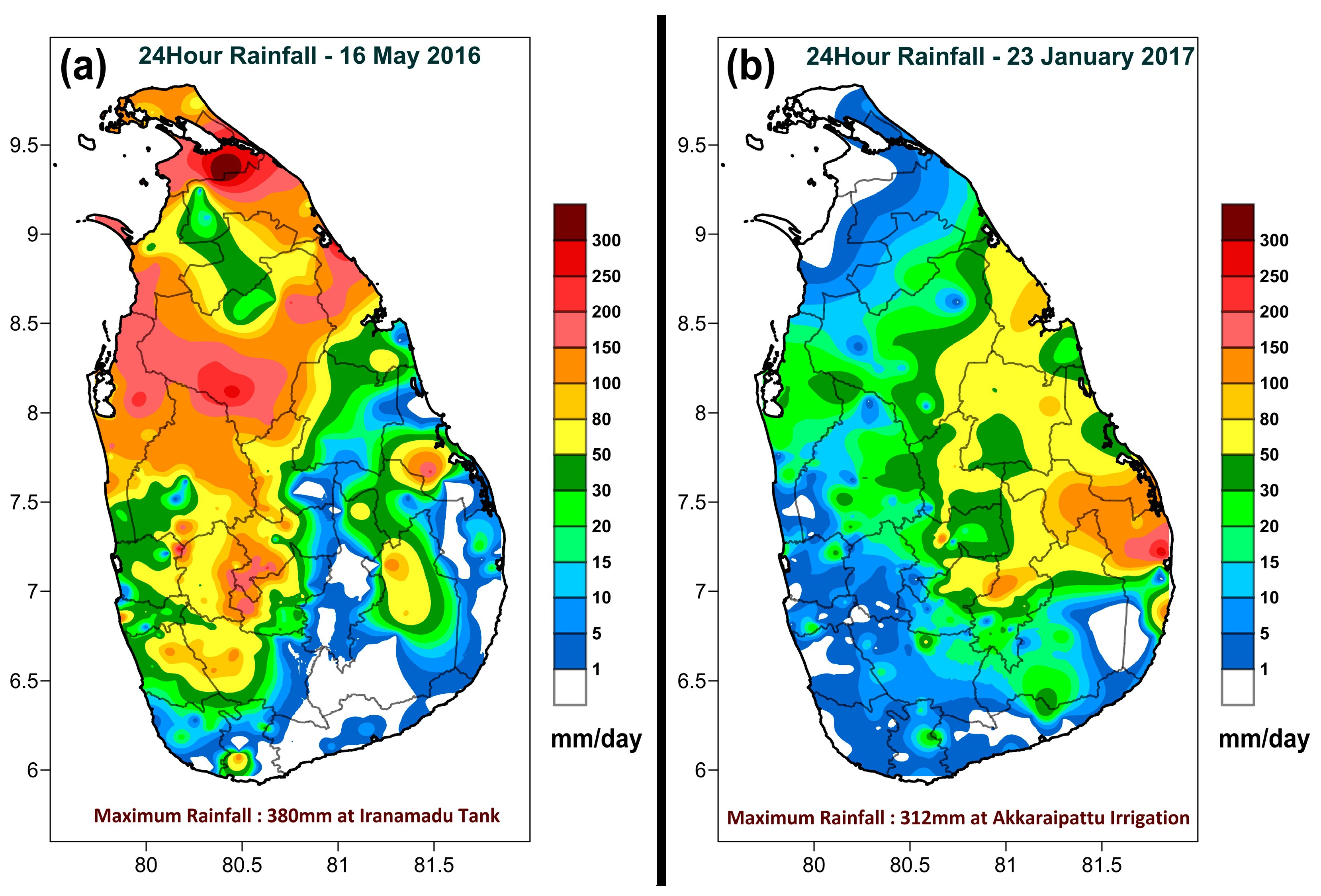
The rainfall events that occurred on 16 May 2016 (Figure 2a) and 23 January 2017 (Figure 2b) were two of the most severe events in recent years. Table 1 shows that the two events corresponded to the southwest monsoon and northeast monsoon seasons in Sri Lanka, respectively. On 16 May 2016, Sri Lanka was affected by a severe tropical storm that caused widespread flooding and landslides in 22 of the 25 districts in the country, destroying dwellings and submerging entire villages. On 23 January 2017, the eastern part of Sri Lanka was affected by heavy rainfall that caused flooding in the Eastern Province.
The atmospheric environment during the southwest monsoon event, which was typical of the southwest season (May), was characterized by an approaching South Asian Monsoon trough over Sri Lanka and a low-pressure system originating to the southeast of the country that resulted in heavy precipitation over the northern and northwestern regions. In this event, because of the onset of the southwest monsoon and the low-pressure system, synoptic scale weather features were more dominant than mesoscale features. The northeast monsoon event (January) was associated with monsoon flow and easterly disturbances during the season that resulted in heavy rainfall over eastern Sri Lanka. Because of the weak northeasterly wind flow and weak large-scale pressure gradient in this event, mesoscale weather features were more dominant than synoptic scale features.
2.2. Method and Materials
The Advanced Research WRF model is a three-dimensional primitive-equation atmospheric circulation model that has been widely utilized to forecast precipitation events. In this study, the WRF model, developed at the National Center of Atmospheric Research (NCAR), was utilized for the sensitivity study for forecasting heavy rainfall in Sri Lanka because the Sri Lanka Administrative Department of Meteorology employs the numerical model for weather and seasonal forecasting.
2.2.1. Basic Model Configuration
To simulate the two heavy rainfall events observed over Sri Lanka, the model version WRF-ARW, which has been employed for operational weather forecasting applications and research studies, was utilized extensively. In this study, The WRF-ARW was configured in the Mercator map projection to represent the land area of Sri Lanka and the surrounding area of the tropical region with a central longitude of 80.78° E and latitude of 7.85° N. The default configuration used a one-way nested domain that consisted an outer domain of 15-km resolution (Figure 3a) and an inner domain of 5-km resolution (Figure 3b), with 100 × 80 and 70 × 106 grid points, respectively. For the static geographical input field, Moderate Resolution Imaging Spectroradiometer 2 (MODIS 2) arc-minutes and 30 arc-second data were used for the outer and inner domain, respectively. The lateral boundary and initial conditions were interpolated from the 0.25 degree (~27 km) Global Forecasting System (GFS) model operated by the National Centers for Environmental Prediction (NCEP). The lateral boundary and initial conditions for the inner nested domain were provided by the output fields of the outer domain produced by the model itself. For the southwest monsoon and northeast monsoon events, model simulations were initialized at the model times/dates of 0000 UTC on 15 May 2016 and 0000 UTC on 22 January 2017 with a 27-h advance from the target period, respectively. The target period for investigation was 24 h. The model simulations in this study focused on rainfall periods of 24 h ending at 0300 UTC, which is the same as the 24-h rainfall criterion used in the Department of Meteorology, Sri Lanka.
For physical parameterization, the default model used the same configuration as that of the WRF-ARW model run by the Numerical Weather Prediction Division in the Department of Meteorology, Sri Lanka. The physical parameterization included the Kain–Fritsch cumulus physics [7], YSU scheme for planetary boundary layers (PBL) [8], WRF Double-Moment 5-class (WDM5) microphysics for the outer domain and WRF Double-Moment 6-class (WDM6) microphysics for the inner domain [9], the Unified Noah land surface model [10], and the Dudhia [11] and RRTM [12] schemes for shortwave and longwave radiation, respectively. Table 2 provides a summary of the default WRF-ARW model configuration and the physical parameterizations for both domains with topographic data. Note that those options for physical parameterization, except for the microphysics schemes, were used for both the outer and inner domain. The initial and boundary conditions for the inner domain were provided by the model results of the outer domain, whose lateral boundary and initial conditions were obtained from the 0.25 degree (~27 km) Global Forecasting System (GFS) model [13] operated by the NCEP.
2.2.2. Experimental Set-up
To evaluate the sensitivity of model horizontal grid resolution and physical parameterizations of the WRF-ARW forecast, model simulations with various configurations were performed for the two selected events being characterized by heavy rainfall occurring in 2016 and 2017 (Table 1). It should be noted that each WRF-ARW model simulation used the same configuration for its initialization, with the exception of different model horizontal resolution and different physical parameterizations. The spin-up time before the model forecasting was 27 h. For the sensitivity test of model resolution to reproduce the targeted rainfalls, we employed two configurations: the default domain configuration with an outer domain with 15-km grid spacing and an inner nested domain with 5-km grid spacing and a new domain configuration with an outer domain with 9-km grid spacing and an inner nested domain with 3-km grid spacing. With the same parameterization schemes given in Table 2, the model performances with the finer outer and inner resolutions were compared to those with the default resolutions.
To evaluate a series of mesoscale simulations with various parameterization schemes, we adopted four different microphysics (MP) schemes, including the WDM5, WDM6, Single-Moment 5-class microphysics (WSM5) [14], and Single-Moment 6-class microphysics (WSM6) [15], and nine different cumulus (CU) parameterizations, including the Kain-Fritsch [7], Old Simplified Arakawa–Schubert [16], Betts–Miller–Janjic [17], Grell–Freitas [18], Multi-scale KF [19], Grell-3 [20], Tiedtke [21], New Tiedtke [22], and New Simplified Arakawa–Schubert [23]. That is, four microphysics schemes, the WSM5, WSM6, WDM5, and WDM6, were configured using the same outer and inner domains for each scheme. For the nine different schemes tested for cumulus parameterization, we used two different methods of configuration of the outer and inner domains, using each scheme for both the inner and outer domain, and using each scheme for only for outer domain with no scheme for the inner domain. For each event, model runs with the 54 combinations of parametrizations were performed. Note that the total number of simulations was 54 × 2 model runs for each event. The numerical results were compared with observations.
2.3. Data
Model output fields were compared with available daily rainfall data from rainfall stations, 3-h synoptic observation data, and radiosonde observation data from weather stations operated by the Department of Meteorology and other institutes in Sri Lanka. The heavy rainfall events described in Table 2 were determined by accessing data from 23 synoptic stations (red squares in Figure 4a), one radiosonde observation (blue star in Figure 4a), and 419 daily rainfall measuring stations (green dots in Figure 4b), which were available for comparison with model predictions, and to evaluate performance. The surface observations were used as ground-truth observations, and the radiosonde observation was used as a true upper air observation. That is, synoptic station data and 24-h rainfall station data were used to evaluate surface model outputs and radiosonde data were used to evaluate upper air temperatures. Among the stations in Figure 4, the radiosonde station with upper-air data observed at 0600 UTC, and the daily rainfall stations measured 24-h rainfall at 0300 UTC each day. Because the WRF-ARW model grid points did not align with the locations of surface and upper air observations, an interpolation method had to be used. This method allowed the data to be aligned so that the variables could be used for comparison with WRF-ARW model predicted outputs.
2.4. Statistical Skill Scores
Once the WRF-ARW model grid point values were interpolated and extracted to each observation location in the horizontal and vertical direction and compared with the data for forecast accuracy, the outputs for each comparison for each day were evaluated qualitatively and quantitatively via statistical skill scores. In statistics, a contingency table provides a basic picture of the interrelation between two variables and helps identify interactions between them [24]. In atmospheric science, the contingency table is one of the methods heavily used for dichotomous categorical verification of forecasts [25]. The data sets were counted into a 2 × 2 contingency table (Table 3), with four elements from YY to NN based on whether an event was observed (YES/NO) and predicted (YES/NO). We employed various statistical evaluations of precipitation indices such as the proportion correct, probability of detection, frequency bias index, threats score, and false alarm ratio. These statistical methods are used widely in data analysis, and the contingency table is useful for assessing the prediction skill of the various indices and for finding appropriate thresholds provided by the categorical verification.
The formulations of the aforementioned statistical skill scores are summarized in Table 4. The frequency bias index (BIAS) is the ratio of the frequency of forecast events to the frequency of observed events. It indicates whether the forecast system has a tendency to under-forecast (BIAS < 1) or over-forecast (BIAS > 1) events, and it measures overall relative frequencies. The value can range between 0 and infinity, and the perfect score is 1. The probability of detection (POD) is the proportion of observed events that were correctly forecast; this is also called the hit rate. The value ranges between 0 and 1 and the perfect score is 1. The threat score (TS), also known as the critical success index, is the fraction of observed and/or forecast events that were predicted correctly. It is concerned only with forecasts that are important, while assuming that correct rejections are not important. It is sensitive to hits and penalizes both misses and false alarms. The value ranges between 0 and 1, and the perfect score is 1. The false alarm ratio (FAR) gives the fraction of forecast events that were observed to be non-events. The value varies between 0 and 1, and the perfect score is 0. The proportion correct (PC) gives the fraction of all forecasts that were correct. It is sensitive to both hits and correct rejections. The value ranges between 0 and 1, and the perfect score is 1.
Table 4 also shows the Pearson correlation coefficient (r), which indicates the strength and direction of a linear relationship between two variables. The Pearson correlation coefficient is obtained by dividing the covariance of the two variables by the product of their standard deviations. If we have a series of N observations and N model values, the correlation coefficient can be used to estimate the correlation between model and observations. The correlation is +1 in the case of a perfect increasing linear relationship and −1 in the case of a perfect decreasing linear relationship, and values in between indicate the degree of linear relationship between, for example, model and observations. A correlation coefficient of 0 means that the there is no linear relationship between the variables. Note that the r values for the model results in this study are between 0 and 1, where the perfect score is 1.
The statistical evaluation method for rainfall occurrence and its amount is very important, and it is necessary to make a combined score in order to compare results. To help summarize the results in this study, it was vital to introduce a combined score from the above statistical scores that could be used together. The combined score was a new skill score created by summarizing the following scores: PC, POD, TS, FAR, and Pearson correlation coefficient, r. The purposes of the combined score were to understand the overall performance better and summarize the results for a final decision.
Combined Score = mean (PC + POD + TS + (1 − FAR) + r)
As shown in Table 4, the values of PC, POD, and TS are always positive and range between 0 and 1. The FAR range is also between 0 and 1. Thus, the result of 1–FAR is always positive and between 0 and 1. Typically, by its definition, the correlation coefficient (r) is between −1 and +1. The combined score and BIAS for evaluation of the model performance are shown in Table 5. These statistical skill scores were used to assess overall performance to determine best model configurations.
3. Results and Discussion
The observations (predictands) match a type of binary scheme, such as precipitation occurrence vs. no precipitation occurrence, and the various parameters as predictors may assume a wide range of values. To evaluate the sensitivity of the horizontal grid of the model and the different physical parameterization schemes, we evaluated model outputs against the surface and upper air observations with selected rainfall thresholds of 50 mm, 100 mm, 125 mm, and 150 mm. To summarize all results related to the rainfall and model physical parameterization, we employed the combined skill score and the BIAS to represent the overall performance of the model rainfall predictions.
3.1. Model Horizontal Resolution
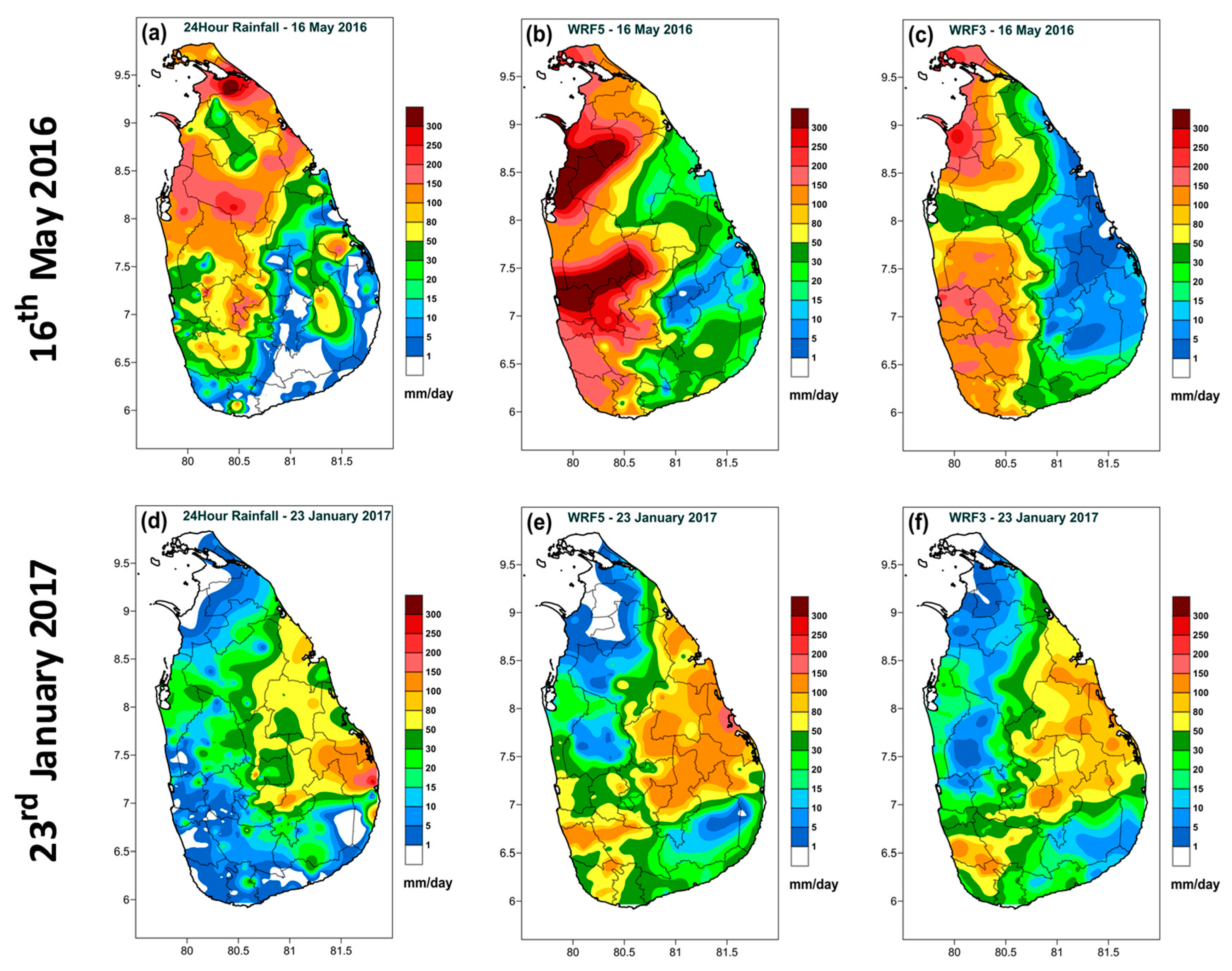
The impact of horizontal grid resolution on WRF-ARW model forecasts, simulating rainfall over Sri Lanka for the two cases of 24 h, was examined at 5-km and 3-km (denoted WRF5 and WRF3) grid spacing (Table 1). Figure 5 shows the observed surface 24-h rainfall (a, d) and the model predicted (b, e), (c, f) rainfall results for 16 May 2016 and 23 January 2017, respectively. Panels (b, e) and (c, f) represent the model simulations for WRF5 and WRF3, respectively.
The observed rainfall on 16 May 2016 (Figure 5a) indicates that the distribution of rainfall was more oriented in the northern and western parts of the island and that the highest rain area was centered in the north of the country. WRF5 (Figure 5b) and WRF3 (Figure 5c) show rainfall distribution similar to observation, except for isolated areas in the eastern part of the country. However, there was a significant difference between the observed rainfall amount and the model simulated rainfall amounts because of model bias, particularly for WRF5 (Figure 5b). WRF3 (Figure 5c) resulted in better simulation than WRF5 (Figure 5b) because it reduced model bias, even though the heavy rainy areas did not match with observation.
For 23 January 2017 (Figure 5d), both WRF5 (Figure 5e) and WRF3 (Figure 5f) accurately identified the rainfall pattern and amount, except for the highest rain area and rainfall in the southwestern part of the country. Similar to the previous case, WRF3 resulted in better simulation than WRF5, reducing model bias and approaching observation.
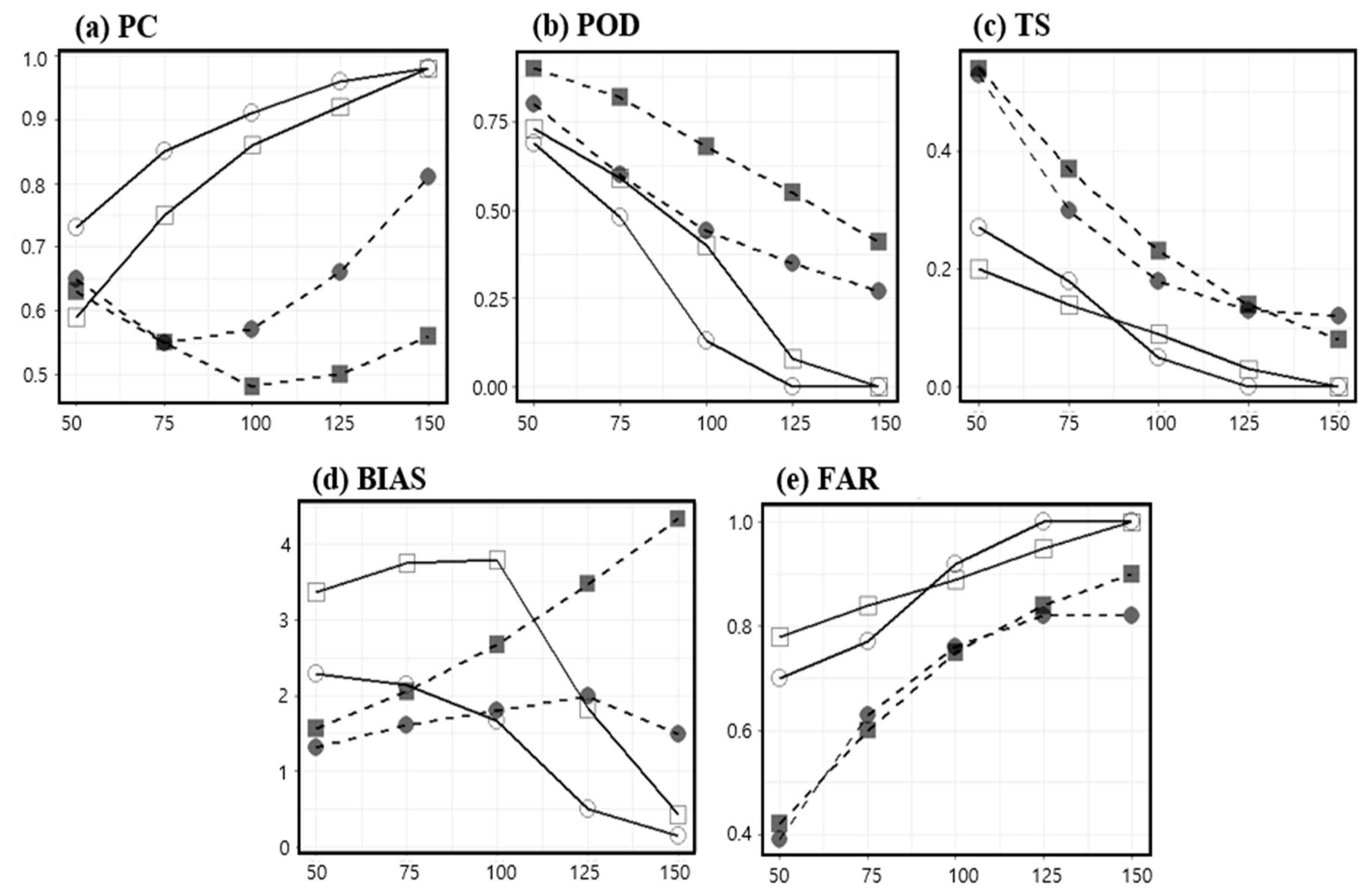
Analysis of the rainfall predictions from the WRF3 experiments showed an overall improvement in the statistical skill scores compared to the WRF5 runs (Figure 6). The PC showed a clear pattern with the events for both model resolutions, while indicating better agreement between observation and model output with WRF3 than with WRF5 (Figure 6a). In both cases, increasing model resolution had an overall positive impact on rainfall prediction. However, according to the POD of rainfall amount exceeding particular thresholds, the WRF5 had slightly higher detection accuracy than the WRF3 (Figure 6b), but the difference was comparatively small, and the patterns were very similar to each other. The TS, which represents the rainfall detection rate together with the false alarm rate, also indicated similar skill for both model resolutions (Figure 6c). BIAS had significant variation in the model predictions with WRF5 for both cases, but WRF3 showed slightly positive and almost stable BIAS for both cases and all rainfall thresholds (Figure 6d). According to the values, WRF5 showed relatively higher positive BIAS (systematic favoring) than the WRF3 model. The FAR did not indicate any significant difference between WRF5 and WRF3 (Figure 6e).
Even though the model resolutions did not show a big difference for predicting rainfall, the results indicated a huge variation with the season. Additionally, when synoptic scale atmospheric features were dominant, the WRF5 and WRF3 models resolved the same weather features much larger than their grid size, simulating them potentially similar with each other. Therefore, the sensitivity of horizontal grid resolution was small, and nearly the same results were produced by both models. However, when mesoscale features were dominant, the model outputs with WRF3 showed better results than the outputs produced by the WRF5 model.
Table 6 shows the skill scores for overall performance, the combined score, and the BIAS, corresponding to the WRF5 (5-km default) and WRF3 (3-km new) simulations. Considering the combined score and BIAS in Table 6, it is clear that increasing the horizontal grid resolution improved the model bias (becoming closer to 1), while the combined scores for rainfall amount and occurrence were similar to each other between the cases. The graphical representations of the model simulations for both heavy rain events shown in Figure 5 also confirmed that positive model bias for rainfall prediction was reduced significantly with the WRF3 (3-km) model configuration, even if the rainfall pattern did not perfectly match observations. Overall, the individual skill scores, combined score, and BIAS for overall performance and the graphical representations confirmed that increasing the horizontal grid resolution from 5 km to 3 km allowed more accurate model output. Previous similar studies for different areas [26,27] also suggested that increasing model resolution has a positive impact for the result in their study area.
3.2. Impact of Physical Parameterization
To investigate the effect of the physical parameterization, the model configured with 3-km resolution for the inner domain and 9-km resolution for the outer domain was selected for sensitivity tests. This selection was made because the model with higher resolution showed better performance than the model with coarser resolution. Figure 7 shows all of the numerical values for combined skill score and BIAS. For the 16 May 2016 event, the combined score values were in the continuous scale of 0.3 to 0.6 (Figure 7a), and the BIAS values were in the continuous scale of 0 to 2.5 (Figure 7b). The combined score and BIAS results for the 23 January 2017 event showed values in the continuous scale from 0 to 0.7 (Figure 7c), and from 0 and 20 (Figure 7d), respectively. Even models have a large variation for predicting rainfall amount while few show good agreement with observations. This clearly indicates that the event of the northeast monsoon (January) had higher correlation between observation and model output than the event of the southwest monsoon (May) season.
There is a strong correlation between the model-simulated rainfalls using WSM5 microphysics with BMJ cumulus physics and WSM6 microphysics with BMJ cumulus physics for the northeast monsoon event, but there is no model simulation showing strong correlation for the event of the southwest monsoon. Among the model simulations, WSM6 microphysics with BMJ cumulus physics and WDM6 microphysics with Old SAS cumulus physics over the outer domain have an acceptable result. According to the skill score of PC, all selected model physics, except for the Grell 3D, Grell–Freitas, and Kain–Fritsch cumulus parameterization schemes, show reasonable scores, but the combinations of BMJ cumulus physics with WSM5, WDM5, and WDM6 microphysics show higher scores than other combinations. The PC scores obtained by using the combinations of New Tiedtke and Old SAS cumulus physics with WSM5, WDM5, and WSM6 microphysics also showed very good agreement with observations.
Additionally, the POD also indicated that using BMJ cumulus physics together with all selected microphysics schemes yielded good scores for the event in May 2016. Among the other cumulus schemes, the Grell 3D, Multi-scale KF, and Old SAS schemes also yielded high scores with all selected microphysics schemes for this event. The Grell 3D and Multi-scale KF cumulus physics schemes together with the WSM5 and WDM5 microphysics schemes produced the highest scores among all combinations of physical parametrizations for the event in January 2017. The combination of BMJ cumulus physics with WSM6 microphysics also showed a good score for the same case. The TS indicated that using the BMJ, Grell 3D, Multi-scale KF, and Old SAS cumulus physics together with WDM5, WSM6, and WDM6 microphysics with the cumulus physics enabled nested domain had high scores for the event on May 2016. Among other cumulus schemes, the New SAS scheme together with WSM6 and WDM6 microphysics using the cumulus physics disabled (explicit) nested domain also showed a significant result. Similarly, using BMJ and Multi-scale KF cumulus physics together with WSM6 microphysics with the cumulus physics enabled nested domain produced the highest scores for the event in January 2017. The same cumulus options together with WSM6 and WDM6 microphysics using the cumulus physics disabled nested domain also showed a good result for the same case.
The model BIAS score indicates whether the models systematically favor producing precipitation. For the case in May 2016, the BIAS scores of several combinations of model physical parameterizations are close to 1 for all rainfall thresholds. Among these, Old SAS cumulus physics together with WDM5, WSM6, and WDM6 microphysics using the cumulus physics enabled nested domain showed comparatively more accurate scores than others for the event in May 2016. The BMJ cumulus physics together with WSM6 microphysics using the cumulus physics enabled nested domain had the most accurate score for the event in January 2017. The skill scores for the FAR for the rainfall simulated by models corresponding to the heavy rain case in May 2016 show similar FAR and a similar pattern with selected rainfall thresholds. However, the FARs corresponding to the heavy rain case in January 2017 clearly indicate a significant result for the combination of BMJ cumulus physics together with WSM5, WDM5, and WSM6 microphysics. The RMSE analysis for model simulated rainfall revealed that the variation in the case of 16 May was comparatively higher than that in the case of 23 January. In the case of 16 May, the cumulus schemes of BMJ, Multi-scale KF, Old SAS, New SAS, Tiedtke, and New Tiedtke together with some microphysical options showed lower values than the others. However, in the case of 23 January, it was clear that BMJ together with all microphysics produced lower RMSE and that the lowest values were obtained with WSM5 and WSM6.
To summarize all of the model physical parameterization results, we utilized the Taylor diagram for the combined skill score and BIAS to represent the overall performance of the model rainfall predictions [28]. Figure 8 shows the results of the combined score and BIAS for 16 May 2016 and 23 January 2017, respectively. The analyzed rainfall predictions for the different physical parameterization schemes revealed that the same model physics had different skills of predicting the two rainfall events. This indicates that the performance of the model physics has a dependency on the season of the event. The variation was significantly smaller for the event in May 2016 (Figure 8a) than the event in January 2017 (Figure 8b). This is a clear indication that the variation of prediction skills among the model physics during the season with dominant large-scale features was quite small compared to that for the season with dominant mesoscale features. Furthermore, some physics schemes showed a very high correlation between model output and observations for the event in January 2017.
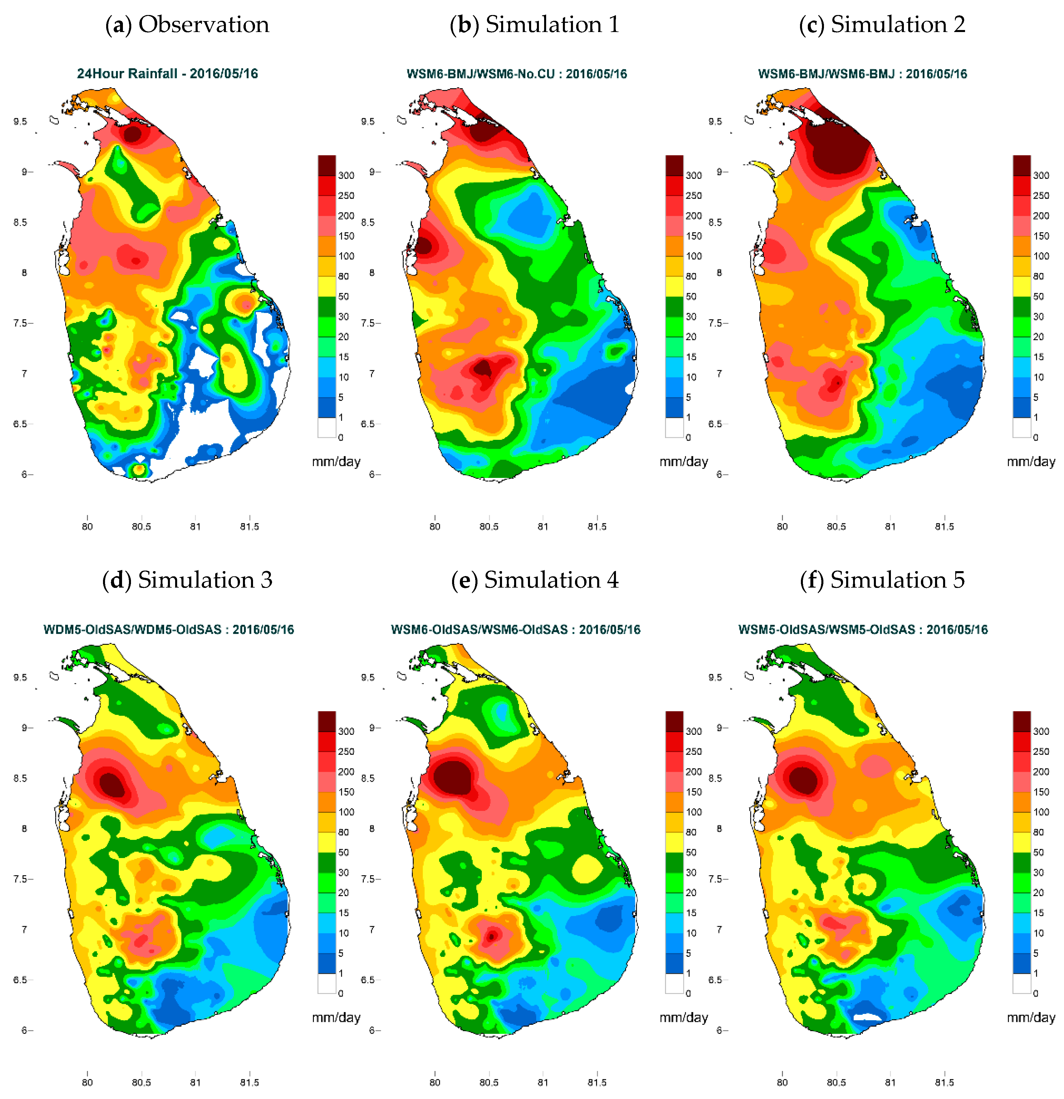
Figure 9 and Figure 10 show daily average rainfalls of observations and the model simulations with the highest five skill scores for the events of 16 May 2016 and 23 January 2017, respectively. For the event of 16 May 2016, the simulations selected are WSM6 microphysics with BMJ cumulus only in the coarse domain (Figure 9b), WSM6 microphysics with BMJ cumulus in both the coarse and fine domains (Figure 9c), WDM5 with Old SAS cumulus in both the coarse and fine domains (Figure 9d), WSM6 with Old SAS cumulus in both the coarse and fine domains (Figure 9e), and WSM5 with Old SAS cumulus in both the coarse and fine domains (Figure 9f). For the event of 23 January 2017, these are WSM6 with BMJ cumulus only in the coarse domain (Figure 10b), WDM6 with Multi-scale KF cumulus only in the coarse domain (Figure 10c), WSM6 with Multi-scale KF cumulus only in the coarse domain (Figure 10d), WSM6 with BMJ cumulus in both the coarse and fine domains (Figure 10e), and WSM5 with BMJ cumulus in both the coarse and fine domains (Figure 10e). For both events, simulation 1 in Figure 9b and Figure 10b, respectively, shows high correlation for the amount and locations of rainfall with the observation in Figure 9a and Figure 10a, respectively.
According to the statistical skill scores and the graphical representations of the model simulations for both heavy rain cases, it was clear that the model outputs showed acceptable predictability for both cases. The model predictions showed high sensitivity with physical parameterization and with atmospheric features during the season. Because each model physical parameterization has its own methods for resolving weather features at different scales, the corresponding results for the heavy rain cases showed seasonal and physical parameterization effects.
4. Summaries and Remarks
The overall results from the sensitivity tests of model horizontal resolution suggest that the WRF-ARW runs using 3-km resolution were marginally better than those using 5-km resolution. Simulations of heavy rainfall with the different physical parameterizations showed significant sensitivity for both microphysics and cumulus schemes, but higher sensitivity for cumulus schemes than microphysics.
The model configurations with the Single-Moment 6-class microphysics (WSM6) scheme, along with the Betts–Miller–Janjic (BMJ) cumulus parameterization scheme used only in the coarse domain with no cumulus in the fine domain, and the WSM6 scheme with the BMJ cumulus parameterization scheme used in both the coarse and fine domains, showed the overall best performances for the case of 16 May 2016 during the southwest monsoon season. Meanwhile, the model configurations with the WSM6 scheme along with the BMJ cumulus parameterization scheme and the Double-Moment 6-class microphysics (WDM6) scheme along with the Multi-scale KF (MKF) cumulus parameterization scheme used only in the coarse domain without a cumulus scheme in fine domain showed the overall best performances for the case of 23 January 2017 during the northeast monsoon season. Therefore, these schemes have potential for operational use for numerical weather prediction in Sri Lanka.
For both case studies, the WRF-ARW model simulations for rainfall were less accurate than their predictions of temperature. More advanced microphysical and cumulus schemes specifically geared toward cloud simulation and precipitation may resolve this issue. The sensitivity results of the physical parameterization schemes did not show a perfect match in any case. However, even though the results indicated that there was large variation in the rainfall estimated by the model using the various model physics schemes, it was also confirmed that several corresponding rainfall simulations were reproduced with spatial distribution aligned with the rainfall station data, although the amount was not estimated accurately.
Finally, the results indicated that the sensitivities of WSM5, WDM5, WSM6, and WDM6 were different. They further showed that the cumulus parameterization is more sensitive than the microphysics for heavy rainfall prediction. The results from previous studies pertaining to the impact of model horizontal resolution on rainfall and the results of this study imply that predictability of rainfall depends on grid resolution, as well as the choice of physical parameterization. The results of this study suggest that more studies of heavy rainfall cases are needed, and that testing more physics schemes, including radiation, boundary layer, and land surface physics, to find better combinations of physics for heavy rainfall forecasting for all seasons would be valuable. However, the quality of the WRF-ARW model predictions are highly dependent on the lateral boundary and initial conditions provided for initialization. Thus, additional sensitivity testing may be needed to determine the sensitivity of a global model data such as ECMWF.
Author Contributions
C.R. and S.K. conceived and designed the experiments, analyzed the data, and wrote the paper. I.H.J. analyzed the numerical results and wrote and edited the paper.
Funding
This research was supported by the Basic Science Research Program through the National Research Foundation of Korea funded by the Ministry of Science, ICT and Future Planning (2017R1E1A1A03070224).
Acknowledgments
The authors thank the editor and reviewers who provided constructive and thoughtful comments to improve this paper.
Conflicts of Interest
The authors declare no conflict of interest.
References
- Hapuarachchi, H.A.S.U.; Jayawardena, I.M.S.P. Modulation of seasonal rainfall in Sri Lanka by ENSO extremes. Sri Lanka J. Meteorol. 2015, 1, 3–11. [Google Scholar]
- Rasmusson, E.M.; Carpenter, T.H. The relationship between eastern equatorial Pacific sea surface temperatures and rainfall over India and Sri Lanka. Mon. Weather Rev. 1983, 111, 517–528. [Google Scholar] [CrossRef]
- Zubair, L.; Ropelewski, C.F. The strengthening relationship between ENSO and Northeast Monsoon rainfall over Sri Lanka and Southern India. J. Clim. 2006, 19, 1567–1575. [Google Scholar] [CrossRef]
- Jayawardene, H.K.W.I.; Sonnadara, D.U.J.; Jayewardene, D.R. Trends of rainfall in Sri Lanka over the last century. Sri Lankan J. Phys. 2005, 6, 7–17. [Google Scholar] [CrossRef]
- Vuillaume, J.F.; Dorji, S.; Komolafe, A.; Herath, S. Sub-seasonal extreme rainfall prediction in the Kelani River basin of Sri Lanka by using self-organizing map classification. Nat. Hazards 2018, 94, 385–404. [Google Scholar] [CrossRef]
- Skamarock, W.C.; Klemp, J.B.; Dudhia, J.; Gill, D.O.; Barker, D.M.; Wang, W.; Powers, J.G. A Description of the Advanced Research WRF Version 3; Technical Report, (June); National Center For Atmospheric Research: Boulder, CO, USA, 2005; p. 113. [Google Scholar]
- Kain, J.S. The Kain-Fritsch convective parameterization: An update. J. Appl. Meteorol. 2004, 43, 170–181. [Google Scholar] [CrossRef]
- Hong, S.-Y.; Noh, Y.; Dudhia, J. A new vertical diffusion package with an explicit treatment of entrainment processes. Mon. Weather Rev. 2006, 134, 2318–2341. [Google Scholar] [CrossRef]
- Lim, K.-S.S.; Hong, S.-Y. Development of an effective double-moment cloud microphysics scheme with prognostic cloud condensation nuclei (CCN) for weather and climate models. Mon. Weather Rev. 2010, 138, 1587–1612. [Google Scholar] [CrossRef]
- Tewari, M.; Chen, F.; Wang, W.; Dudhia, J.; LeMone, M.A.; Mitchell, K.; Ek, M.; Gayno, G.; Wegiel, J.P.; Cuenca, R.H. Implementation and verification of the unified noah land surface model in the WRF model. Bull. Am. Meteorol. Soc. 2004, 27, 2165–2170. [Google Scholar] [CrossRef]
- Dudhia, J. Numerical study of convection observed during the winter monsoon experiment using a mesoscale two-dimensional model. J. Atmos. Sci. 1989, 3077–3107. [Google Scholar] [CrossRef]
- Mlawer, E.J.; Taubman, S.J.; Brown, P.D.; Iacono, M.J.; Clough, S.A. Radiative transfer for inhomogeneous atmospheres: RRTM, a validated correlated-k model for the longwave. J. Geophys. Res. Atmos. 1997, 102, 16663–16682. [Google Scholar] [CrossRef] [Green Version]
- NCEP. The GFS Atmospheric Model, Note 442., (November); NCEP: Washington, DC, USA, 2003; p. 14. Available online: http://www.emc.ncep.noaa.gov/officenotes/newernotes/on442.pdf (accessed on 30 June 2017).
- Hong, S.-Y.; Dudhia, J.; Chen, S.-H. A revised approach to ice microphysical processes for the bulk parameterization of clouds and precipitation. Mon. Weather. Rev. 2004, 132, 103–120. [Google Scholar] [CrossRef]
- Hong, S.; Lim, J. The WRF single-moment 6-class microphysics scheme (WSM6). J. Korean Meteorol. Soc. 2006, 42, 129–151. [Google Scholar]
- Pan, H.-L.; Wu, W.-S. Implementing a mass flux convective parameterization package for the NMC medium-range forecast model. NMC Off. Note 1995, 409. Available online: http://www.emc.ncep.noaa.gov/officenotes/FullTOC.html (accessed on 27 September 2017).
- Janjić, Z.I. The Step-Mountain Eta Coordinate Model: Further developments of the convection, viscous sublayer, and turbulence closure schemes. Mon. Weather Rev. 1994, 927–945. [Google Scholar] [CrossRef]
- Grell, G.A.; Freitas, S.R. A scale and aerosol aware stochastic convective parameterization for weather and air quality modeling. Atmos. Chem. Phys. 2014, 14, 5233–5250. [Google Scholar] [CrossRef] [Green Version]
- Kain, J.S.; Fritsch, J.M. Multiscale convective overturning in mesoscale convective systems: Reconciling observations, simulations, and theory. Mon. Weather. Rev. 1998, 126, 2254–2273. [Google Scholar] [CrossRef]
- Grell, G.A.; Dévényi, D. A generalized approach to parameterizing convection combining ensemble and data assimilation techniques. Geophys. Res. Lett. 2002, 29. [Google Scholar] [CrossRef]
- Tiedtke, M. A comprehensive mass flux scheme for cumulus parameterization in large-scale models. Mon. Weather Rev. 1989, 117, 1779–1800. [Google Scholar] [CrossRef]
- Zhang, C.; Wang, Y.; Hamilton, K. Improved representation of boundary layer clouds over the southeast Pacific in ARW-WRF using a modified Tiedtke cumulus parameterization scheme. Mon. Weather Rev. 2011, 139, 3489–3513. [Google Scholar] [CrossRef]
- Han, J.; Pan, H.-L. Revision of convection and vertical diffusion schemes in the NCEP Global Forecast System. Weather Forecast. 2011, 26, 520–533. [Google Scholar] [CrossRef]
- Pearson, K. On the Theory of Contingency and Its Relation to Association and Normal Correlation; Drapers’ Company Research Memoirs Biometric Series I; Cambridge University Press: Cambridge, UK, 1904. [Google Scholar]
- Wilks, D.S. Statistical Methods in the Atmospheric Sciences; Academic Press: San Diego, CA, USA, 1995. [Google Scholar]
- Done, J.; Davis, C.A.; Weisman, M. The next generation of NWP: Explicit forecasts of convection using the weather research and forecasting (WRF) model. Atmos. Sci. Lett. 2004, 5, 110–117. [Google Scholar] [CrossRef]
- Wang, W.; Seaman, N.L. A comparison study of convective parameterization schemes in a mesoscale model. Mon. Weather Rev. 1997, 125, 252–278. [Google Scholar] [CrossRef]
- Taylor, K.E. Summarizing multiple aspects of model performance in a single diagram. J. Geophys. Res. 2001, 106, 7183–7192. [Google Scholar] [CrossRef] [Green Version]
Figure 1.
(a) Location of Sri Lanka on the world map. (b) Topographic elevation in Sri Lanka. The orange rectangle in (a) indicates the location of Sri Lanka in the Indian Ocean.
Figure 1.
(a) Location of Sri Lanka on the world map. (b) Topographic elevation in Sri Lanka. The orange rectangle in (a) indicates the location of Sri Lanka in the Indian Ocean.

Figure 2.
Daily average rainfall on (a) 16 May 2016 and (b) 23 January 2017.

Figure 3.
Numerical model (a) outer domain of 15 km shown by yellow outside rectangle and (b) inner domain of 5 km shown by inside yellow rectangule in (a).
Figure 3.
Numerical model (a) outer domain of 15 km shown by yellow outside rectangle and (b) inner domain of 5 km shown by inside yellow rectangule in (a).
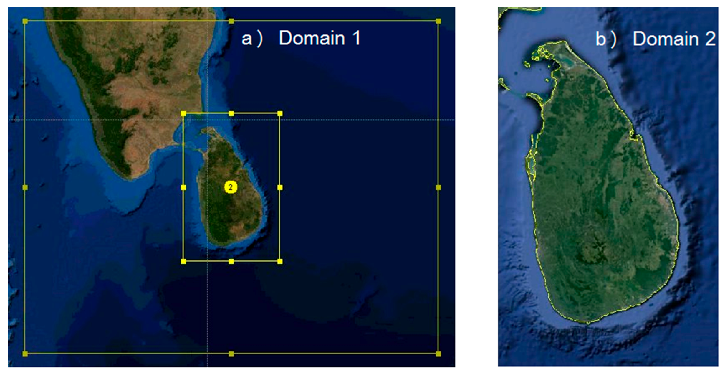
Figure 4.
Measurement location map in Sri Lanka for (a) radiosonde station (blue star) and synoptic stations (red squares) and (b) daily rainfall observation stations (green dots).
Figure 4.
Measurement location map in Sri Lanka for (a) radiosonde station (blue star) and synoptic stations (red squares) and (b) daily rainfall observation stations (green dots).
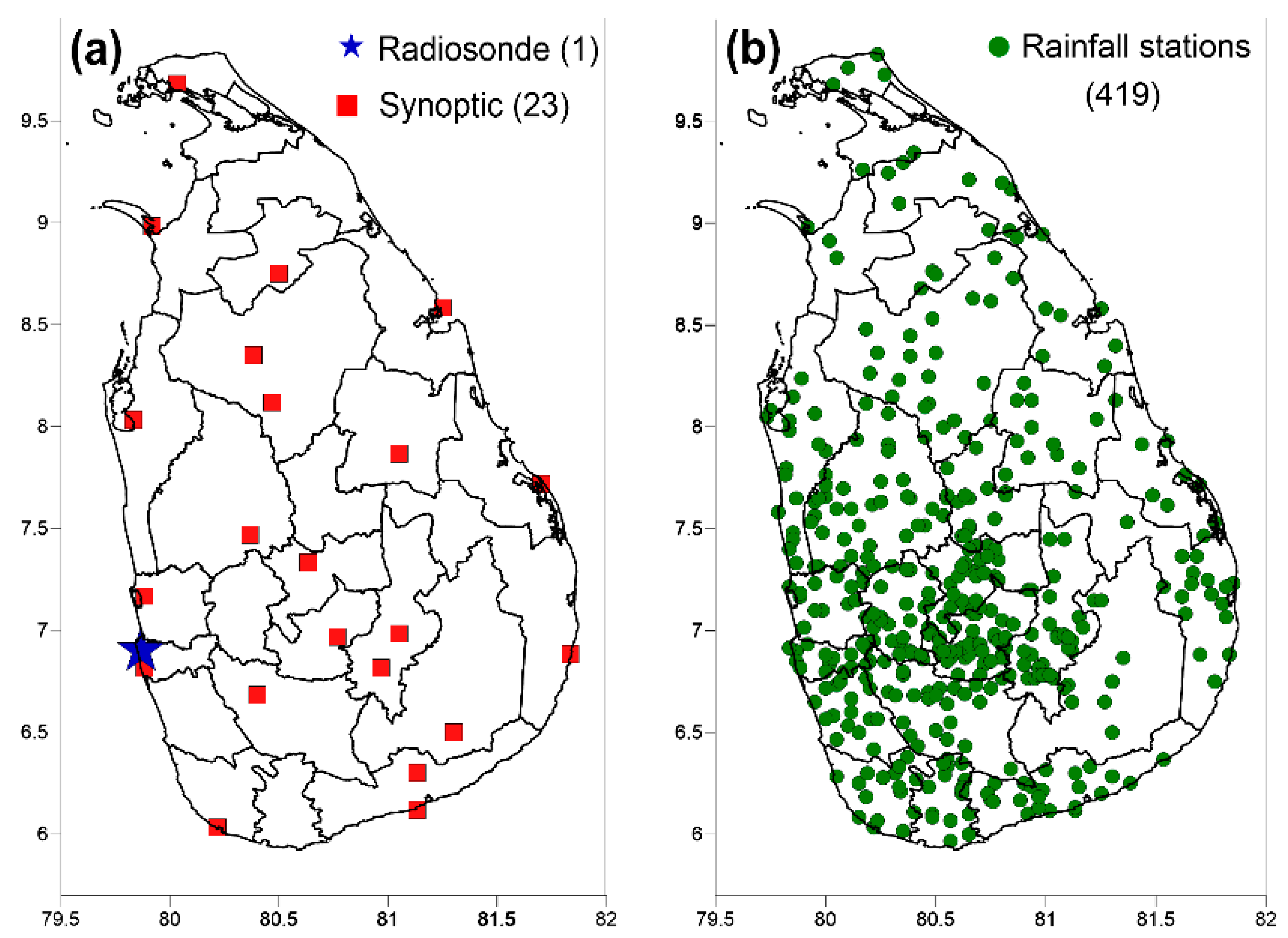
Figure 5.
Daily averaged rainfall for observations (a,d) and model predictions of WRF5 (b,e) and WRF3 (c,f) on 16 May 2016 and 23 January 2017, respectively. Color bar represents the amount of rainfall in the unit of mm/day.
Figure 5.
Daily averaged rainfall for observations (a,d) and model predictions of WRF5 (b,e) and WRF3 (c,f) on 16 May 2016 and 23 January 2017, respectively. Color bar represents the amount of rainfall in the unit of mm/day.

Figure 6.
Statistical skill scores for (a) proportion correct (PC); (b) probability of detection (POD); (c) threat score (TS); (d) frequency bias index (BIAS); and (e) false alarm ratio (FAR). The white (black) circles and white (black) squares connected with solid (dashed) lines represent the statistical values for the event of 23 January 2017 (16 May 2016). The circles and squares indicate the statistical results for WRF3 and WRF5, respectively. The x-axis represents the rainfall threshold (mm/day).

Figure 7.
Combined Skill score (a,c) and BIAS (b,d) for the events of (a,b) 16 May 2016 and (c,d) 23 January 2017. The descrete microphysical schemes along the horizontal axis are WSM5, WDM5, WSM6-1 (WSM6 with CP in both domains), WSM6-2 (WSM6 without CP in the fine domain), WDM6-1 (WDM6 with CP in both domains), and WDM6-2 (WDM6 without CP in the fine domain). The shapes ( ![Atmosphere 09 00378 i001]() ,
, ![Atmosphere 09 00378 i002]() ,
, ![Atmosphere 09 00378 i003]() ,
, ![Atmosphere 09 00378 i004]() , O,
, O, ![Atmosphere 09 00378 i005]() ,
, ![Atmosphere 09 00378 i006]() ,
, ![Atmosphere 09 00378 i007]() ,
, ![Atmosphere 09 00378 i008]() ) indicate KF, BMJ, New SAS, Grell 3D, Old SAS, Grell–Freitas, Kain–Fritch, NEW SAS, and Multi-scale KF, respectively.
) indicate KF, BMJ, New SAS, Grell 3D, Old SAS, Grell–Freitas, Kain–Fritch, NEW SAS, and Multi-scale KF, respectively.
 ,
,  ,
,  ,
,  , O,
, O,  ,
,  ,
,  ,
,  ) indicate KF, BMJ, New SAS, Grell 3D, Old SAS, Grell–Freitas, Kain–Fritch, NEW SAS, and Multi-scale KF, respectively.
Figure 7.
Combined Skill score (a,c) and BIAS (b,d) for the events of (a,b) 16 May 2016 and (c,d) 23 January 2017. The descrete microphysical schemes along the horizontal axis are WSM5, WDM5, WSM6-1 (WSM6 with CP in both domains), WSM6-2 (WSM6 without CP in the fine domain), WDM6-1 (WDM6 with CP in both domains), and WDM6-2 (WDM6 without CP in the fine domain). The shapes ( ![Atmosphere 09 00378 i001]() ,
, ![Atmosphere 09 00378 i002]() ,
, ![Atmosphere 09 00378 i003]() ,
, ![Atmosphere 09 00378 i004]() , O,
, O, ![Atmosphere 09 00378 i005]() ,
, ![Atmosphere 09 00378 i006]() ,
, ![Atmosphere 09 00378 i007]() ,
, ![Atmosphere 09 00378 i008]() ) indicate KF, BMJ, New SAS, Grell 3D, Old SAS, Grell–Freitas, Kain–Fritch, NEW SAS, and Multi-scale KF, respectively.
) indicate KF, BMJ, New SAS, Grell 3D, Old SAS, Grell–Freitas, Kain–Fritch, NEW SAS, and Multi-scale KF, respectively.
, , , , O, , , , ) indicate KF, BMJ, New SAS, Grell 3D, Old SAS, Grell–Freitas, Kain–Fritch, NEW SAS, and Multi-scale KF, respectively.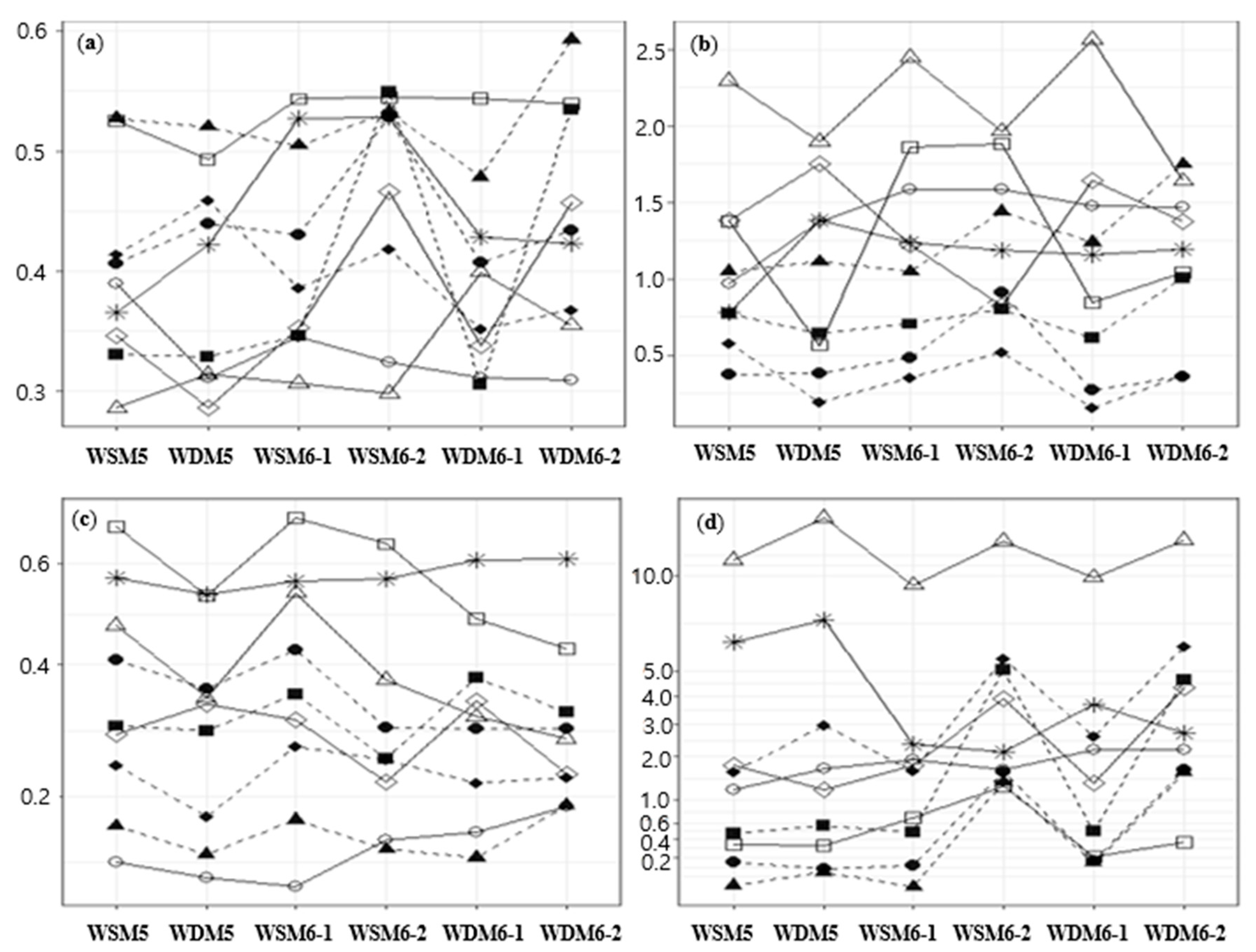
Figure 8.
Taylor diagram displaying combined skill score and BIAS for the events of (a) 16 May 2016 and (b) 23 January 2017. The red dot indicates the most accurate location for the combined skill and BIAS. Other dots indicate the locations of model results for combined skill and BIAS.
Figure 8.
Taylor diagram displaying combined skill score and BIAS for the events of (a) 16 May 2016 and (b) 23 January 2017. The red dot indicates the most accurate location for the combined skill and BIAS. Other dots indicate the locations of model results for combined skill and BIAS.

Figure 9.
24-h rainfall on 16 May 2016 for observation (a) and model predictions representing the model simulations using the selected (optimum configurations by graphical representation) microphysical and cumulus parameterization schemes: (b) WSM6 microphysics with BMJ cumulus only in the coarse domain, (c) WSM6 microphysics with BMJ cumulus in both the coarse and fine domains, (d) WDM5 microphysics with Old SAS cumulus in both the coarse and fine domains, (e) WSM6 microphysics with Old SAS cumulus in both the coarse and fine domains, and (f) WSM5 microphysics with Old SAS cumulus in both the coarse and fine domains.

Figure 10.
24-h rainfall on 23 January 2017 for observation (a) and model predictions representing the model simulations using the selected (optimum configurations by graphical representation) microphysical and cumulus parameterization schemes: (b) WSM6 microphysics with BMJ cumulus only in the coarse domain, (c) WDM6 microphysics with Multi-scale KF cumulus only in the coarse domain, (d) WSM6 microphysics with Multi-scale KF cumulus only in the coarse domain, (e) WSM6 microphysics with BMJ cumulus in both the coarse and fine domains, and (f) WSM5 microphysics with BMJ cumulus in both the coarse and fine domains.


Table 1.
Summary of selected rainfall cases.
| Event | Date/Time | Season | Duration (hours) | Max. 24-h Rainfall (mm) |
|---|---|---|---|---|
| 1 | 0300 UTC 16 May–0300 UTC 17 May 2016 | Southwest monsoon | 24 | 380 |
| 2 | 0300 UTC 23 January–0300 UTC 24 January 2017 | Northeast monsoon | 24 | 312 |
Table 2.
Default model configuration and physical parameterization.
| Configuration | Outer Domain | Inner Domain |
|---|---|---|
| WRF version | 3.8.1 | |
| Horizontal grids | 100 × 80 | 70 × 106 |
| Grid spacing (km) | 15 | 5 |
| Vertical grids | 42 layer/Top 50 hPa | |
| Integration time (s) | 90 | 30 |
| Radiation | Dudhia shortwave/RRTM longwave Integration time: 10 min | |
| Microphysics | WDM 5-class | WDM 6-class |
| Surface layer | MM5 Similarity scheme | |
| Land surface | Unified Noah LSM | |
| Planetary boundary layer | Yonsei University (YSU) scheme Integration time: every time step | |
| Land use and topography data | 2 m/MODIS 21 | 30 s/MODIS 21 |
| Cumulus | Kain–Fritsch scheme | |
| Initial boundary condition | Global Forecasting System (GFS) Model Forecast Fields (27 km resolution, NCEP) | |
Table 3.
Contingency table for a dichotomous categorical verification of forecasts.
| Observed | ||||
|---|---|---|---|---|
| Yes | No | |||
| Forecast | Yes | Hits (YY) | False alarms (YN) | # (Forecast yes) |
| No | Misses (NY) | Correct rejections (NN) | # (Forecast no) | |
| # (observed yes) | # (observed no) | Total = N | ||
#: counts of ().
Table 4.
Summary of statistical skill scores for evaluating the model performance. Xi is observed values and Yi is modeled values.
Table 4.
Summary of statistical skill scores for evaluating the model performance. Xi is observed values and Yi is modeled values.
| Variable | Evaluation Method | Formula | Range | Perfect Score |
|---|---|---|---|---|
| Rainfall occurrence | Frequency bias index (BIAS) | 0~ | 1 | |
| Probability of detection (POD) | 0~1 | 1 | ||
| Threat score (TS) | 0~1 | 1 | ||
| False alarm ratio (FAR) | 0~1 | 0 | ||
| Proportion correct (PC) | 0~1 | 1 | ||
| Rainfall amount | Pearson correlation coefficient (r) | −1~1 | 1 |
Table 5.
Summary of statistics for evaluating overall performance.
| Evaluation Method | Range | Perfect Score | |
|---|---|---|---|
| Overall performance of rainfall prediction | Combined score | −0.2~1 | 1 |
| BIAS | 0~∞ | 1 |
Table 6.
Summary of combined score and BIAS (bias index) for overall performance.
| Rainfall Event | 5-km (Default) Configuration | 3-km (New) Configuration | ||
|---|---|---|---|---|
| Combined Score | BIAS | Combined Score | BIAS | |
| 16 May 2016 | 0.35 | 2.82 | 0.34 | 1.64 |
| 23 Jan 2017 | 0.31 | 2.64 | 0.34 | 1.35 |
© 2018 by the authors. Licensee MDPI, Basel, Switzerland. This article is an open access article distributed under the terms and conditions of the Creative Commons Attribution (CC BY) license (http://creativecommons.org/licenses/by/4.0/).
Share and Cite
MDPI and ACS Style
Rodrigo, C.; Kim, S.; Jung, I.H. Sensitivity Study of WRF Numerical Modeling for Forecasting Heavy Rainfall in Sri Lanka. Atmosphere 2018, 9, 378. https://doi.org/10.3390/atmos9100378
AMA Style
Rodrigo C, Kim S, Jung IH. Sensitivity Study of WRF Numerical Modeling for Forecasting Heavy Rainfall in Sri Lanka. Atmosphere. 2018; 9(10):378. https://doi.org/10.3390/atmos9100378
Chicago/Turabian StyleRodrigo, Channa, Sangil Kim, and Il Hyo Jung. 2018. "Sensitivity Study of WRF Numerical Modeling for Forecasting Heavy Rainfall in Sri Lanka" Atmosphere 9, no. 10: 378. https://doi.org/10.3390/atmos9100378
Note that from the first issue of 2016, this journal uses article numbers instead of page numbers. See further details here.