Influence of Disdrometer Type on Weather Radar Algorithms from Measured DSD: Application to Italian Climatology

Abstract

Relations for retrieving precipitation and attenuation information from radar measurements play a key role in radar meteorology. The uncertainty in such relations highly affects the precipitation and attenuation estimates. Weather radar algorithms are often derived by applying regression methods to precipitation measurements and radar observables simulated from datasets of drop size distributions (DSD) using microphysical and electromagnetic assumptions. DSD datasets can be derived from theoretical considerations or obtained from experimental measurements collected throughout the years by disdrometers. Although the relations obtained from experimental disdrometer datasets can be generally considered more representative of a specific climatology, the measuring errors, which depend on the specific type of disdrometer used, introduce an element of uncertainty to the final retrieval algorithms. Eventually, data quality checks and filtering procedures applied to disdrometer measurements play an important role. In this study, we pursue two main goals: (i) evaluate two different techniques for establishing weather radar algorithms from measured DSD, and (ii) investigate to what extent dual-polarization radar algorithms derived from experimental DSD datasets are influenced by the different error structures introduced by the various disdrometer types (namely 2D video disdrometer, first and second generation of OTT Parsivel disdrometer, and Thies Clima disdrometer) used to collect the data. Furthermore, weather radar algorithms optimized for Italian climatology are presented and discussed.

1. Introduction

Networks of ground-based weather radars are widely used worldwide to obtain quantitative precipitation estimations (QPEs) over large areas with fairly high temporal (5–10 min) and spatial resolution (usually less than 1 km, although variable with the distance from the radar). In Italy, the national weather radar network is managed by the Italian Civil Protection Department, and most of its systems operate in dual polarization mode with polarization diversity, thus making it possible to improve the retrieval of precipitation with important consequences in different fields, such as management of hydrological risk, understanding of water cycle and ultimately investigation of the effects of climate change. However, weather radar data are indirect measurements of rainfall, and therefore proper radar relationships (retrieval algorithms) are often used to convert combinations of radar measurements into rainfall rate, parameters characterizing drop size distribution (DSD), or specific attenuation. In radar meteorology, the most used radar rainfall retrieval algorithm is the one that converts the equivalent reflectivity factor, usually at horizontal polarization (Z_h in dB) measured by a radar system, into rainfall rate (R in mm h⁻¹) using a power law relation of the form $R=c_1{Z_h}^{c_2}$ [1]. This relation is often tuned by statistical matching between radar-measured reflectivity factor and raingauge-measured rainfall accumulations [2]. However, because of the drop size distribution (DSD) variability even at close distances [3] and differences in the sampling volume of the devices, the parameters (c₁ and c₂) of the Z_h vs. R relation are highly variable [4]. The use of dual polarization radar measurements such as differential reflectivity (Z_dr in dB) and the specific differential phase shift (K_dp in ° km⁻¹) can better constrain some features of the DSD and consequently improve the QPE, providing relations less sensitive to variation of DSD [2,5]. Furthermore, when precipitation-attenuated frequencies are used, relations between radar measurements and the specific attenuation or differential attenuation (a_h and a_d, respectively, and both in dB km⁻¹) are needed in order to apply attenuation correction algorithms and obtain more reliable radar measurements [6].

Following the classification proposed in [2], radar rainfall estimation techniques can be classified as either statistically based or physically based. The techniques adopting a statistical approach define rainfall algorithms analyzing rain measurements and corresponding radar measurements collected aloft by radar. The physically based techniques require a microphysical model of rain coupled with an electromagnetic model for scattering and absorption to determine how radar observations are related to rain within a radar resolution volume. In practice, they lead to approximated parametric relations between rain and radar measurements, typically expressed through power laws whose parameters are obtained starting from a set of drop size distributions. For each DSD in the set, using additional assumptions that will be discussed later, rain rate and simulated radar measurements are obtained. Parameters of the approximated relations are determined through a non-linear regression analysis. DSD variability is one of the primary sources of error of radar QPE algorithms, especially for algorithms based only on reflectivity measurements. Therefore, the choice of the set of DSDs is important for training radar-based algorithms for rain precipitation and attenuation estimation. Two methods are generally adopted for the selection of the DSD dataset: one is based on drop size distributions measured by surface devices (such as disdrometers), and the other is structured around sets of synthetic DSDs either generated by varying the parameters of an assumed theoretical functional form [2], or more often obtained by fitting the measured DSD with a given model (e.g., [7], among others). Usually the three-parameter gamma distribution is adopted as the theoretical distribution able to represent the natural variability of rain. The latter approach assumes that the radar system always samples raindrops whose sizes follow a gamma distribution (homogeneous within the radar sample volume), from which both DSD moments (such as rain rate) and radar measurements can be computed. However, the use of an a priori analytical DSD model (such as the gamma) could lead to errors in weather radar algorithms. For instance, Ref. [8] pointed out that the gamma DSD assumption can influence the radar rain rate estimation and, more recently, Refs. [9,10] investigated the validity of three common used distributions to model the natural DSDs through evaluation of the goodness of fit for large disdrometric databases. Moreover, the method used to fit a given functional form to the measured DSD produces an estimation error that can influence the performance of the obtained weather radar algorithms. For example, Ref. [11] demonstrated that the method of moments, which is widely used for DSD parameter estimation, produced biased parameters, and the maximum likelihood or L-moments methods perform better. Disdrometers are becoming more popular, and long-term measurements of DSD are available and can be used to determine physically based rain algorithms. On the other hand, considering disdrometer-measured DSDs avoids uncertainties related to the assumption of a specific DSD functional form; however, disdrometer-estimated DSDs will have error that, in turn, will have an impact on rain radar algorithms. In general, for physically based techniques, other factors, such as radar measurement fluctuations, e.g., [12], sampling effects, e.g., [13,14], and other assumptions such as the shape of the raindrops, e.g., [15], usually modelled as oblate spheroids, have to be taken into account. Ref. [16] provides a review of the main techniques used to retrieve precipitation from remote sensing measurements. Another important advantage in using experimental DSD is that the obtained algorithms are optimized for the climate region in which the disdrometer measurements have been collected, whereas less customized algorithms are obtained using synthetic DSDs. Similar considerations can be made for the relations between radar measurements and specific attenuation as well, that is not directly measured by a radar, but is used in some QPE techniques when C- or X-band frequencies, suffering from rain attenuation, are used.

Important aspects to be considered in using experimental DSDs to determine weather radar algorithms are (i) the spurious variability of measured DSDs due to instrumental and observational noise, and (ii) the error structure of the measured drop spectra in relation to the kind of device used for the measurements. The first aspect has been partially addressed by [17], who investigated the effect of the sequential intensity filtering technique (SIFT) to obtain more stable R-Z_h relation. Ref. [18] defined another sorting and averaging methods to reduce the disdrometer sampling error based on two DSD moments (namely rainfall rate and median volume diameter), the so-called SATP method. In the present study, the SIFT approach is used to establish different types of weather radar algorithms, and the results are compared with the relations obtained from the classical approach using 1-min disdrometer DSDs. The second aspect is the aim of this study and has never been addressed systematically in the literature, with the exception of a very recent study ([19]) that compares the performance of laser disdrometer Parsivel2 by OTT GmbH and Joanneum Research 2D Video Disdrometer (2DVD), installed in South Korea, in estimating precipitation radar algorithms at S-band. In fact, disdrometer data are often considered as “ground truth” for the measurements of DSD at ground and in practice are used acritically for the determination of weather radar algorithms. Sometimes they are preferred to standard raingauge as a reference for ground measurements of rainfall especially for light precipitation ([20]), and therefore are not only DSD estimation instruments. However, a WMO experiment for raingauge intercomparison showed a 15% bias with respect to raingauges ([21]) for both an OTT Parsivel disdrometer and a Thies Clima LPM (Laser Precipitation Monitor) in the estimation of rainfall intensity. In general, disdrometers can be affected by several errors, which are caused by: (i) statistical sampling (e.g., [22,23]), (ii) instrument limitations (resolution and sensitivity), and (iii) environmental factors such as wind effect (e.g., [24,25]), splashing (e.g., [7]) or external interference from, for instance, insects or spider webs. Errors due to instrumental limitations (referred to as error structure above) depend on the type of disdrometer and the measurement principle adopted and can affect the measured DSD in different ways. Nowadays, different kind of devices are commercially available. Based on their measurement principle, they can be classified in three categories: impact-type, laser, and video. Several authors have compared measurements of different disdrometers and have found systematic differences in the shape of measured drop spectra and corresponding integral parameters (e.g., [7,26,27,28,29] among others).

In this study, we investigate to what extent differences in DSD estimated by different types of disdrometer can impact the determination of weather radar algorithms. In other words, we aim at understanding and quantifying how the different characteristics, sensitivities and measurement modes of disdrometers influence the coefficients of the parametric algorithms adopted for the retrieval of rainfall rate and attenuation from radar measurements.

Once the impact of the type of disdrometer on the weather radar algorithms has been carefully addressed and examined based on data from experimental campaigns, the DSDs collected by a quality-controlled Thies Clima optical disdrometer over five years in Rome (Italy) are analyzed in order to provide polarimetric weather radar algorithms optimized for the Mediterranean region.

This study is focused on the most used weather radar algorithms for radar-based QPE and specific attenuation estimation. The obtained relations are provided for the three frequencies of the bands (S, C and X) that are commonly adopted for ground-based weather radars. The rest of the paper is organized as follows. Section 2 describes the main characteristics of the disdrometers considered in this study and of the measured datasets involved in the analysis. Section 3 reports the methods adopted to define the weather radar algorithms. Section 4 deals with the influence of the measuring characteristics of the different types of disdrometers on the parameters of the weather radar algorithms. The dual-polarization weather radar algorithms optimized for Italy are presented in Section 5. Finally, Section 6 closes the paper by summarizing and commenting on the main results.

2. Devices and Datasets Description

2.1. Experimental Data

The experimental data used in this study was collected by four types of commonly used disdrometers: Parsivel disdrometer (P1), Parsivel2 disdrometer (P2), which is an upgraded version of P1, both manufactured by OTT Hydromet GmbH (Kempten, Germany), Thies Clima laser precipitation monitor (TC), manufactured by Adolf Thies GmbH & Co. KG (Göttingen, Germany), and 2D Video Disdrometer (2DVD), by Johanneum Research GmbH (Graz, Austria). The data used were mainly collected in the area of Rome (Italy), but disdrometer measurements collected in Iowa (USA) were also considered to enrich the analysis of the effect of the disdrometer type on the weather radar algorithms (Figure 1). In Rome, data collected over roughly 5 years by a P1 and TC installed on the roof of the Institute of Atmospheric Sciences and Climate (ISAC) of the National Research Council (CNR) were used (hereafter ISAC-CNR P1 and ISAC-CNR TC, respectively). To the best of the authors’ knowledge, the latter represent the longest DSD datasets available in Italy. Furthermore, during the two-month Hydrological cycle in Mediterranean Experiment (HyMeX) Special Observation Period 1 (SOP1) field campaign from September to November 2012 [30], P2 and 2DVD (hereafter HyMeX P2 and HyMeX 2DVD respectively) were made available by the National Aeronautics and Space Administration (NASA) thanks to a specific agreement to support such a field campaign. A P2 disdrometer was deployed next to P1 and TC on the ISAC roof, and one 2DVD was located on the roof of the Department of Electrical Engineering and Telecommunications at Sapienza University of Rome (14 km from ISAC-CNR; [31]). In Iowa, during the Iowa Flooding Studies (IFloodS) field campaign of the NASA ground validation program of the Global Precipitation Measurement (GPM) mission, six different sites aligned along a fixed direction were equipped with one 2DVD and one P2, and the data are available online (hereafter IFloodS 2DVD and IFloodS P2, respectively; [32,33]). Furthermore, only for comparison purposes (see Section 4), we built three new datasets as subsets of the long-term ones, namely, ISAC-CNR P1 and ISAC-CNR TC. The rationale for this decision is to quantify the possible effect of the duration of the period during which the data were collected. Specifically, ISAC-CNR P1_sub and ISAC-CNR TC_sub denote subsets of the long-term datasets ISAC-CNR P1 and ISAC-CNR TC, respectively, and consist of two months of data (from 24 September to 30 November 2015) during which both of the devices collected data simultaneously. Furthermore, ISAC-CNR TC_HY denotes the data collected by TC during the HyMeX field campaign, and therefore it is another subset of the ISAC-CNR TC dataset. Figure 1 shows the locations in Italy and Iowa of the devices used in this study, and

Table 1. For each dataset, provided are the type of device, the location, the time period when measurements were collected, the total number of rainy minutes considered after the application of the filtering, the mean and maximum values of the rainfall rate and the percentage of minutes classified as Convective (C), or Stratiform (S), applying the [40] classification algorithm.

Dataset Name	Type of Device	Location	Time Period	n. Rainy Min.	Rmean (mm h−1)	Rmax (mm h−1)	% C	% S
ISAC-CNR P1	P1	Rome, IT	June 2010–March 2016	82,792	2.25	133.4	3.58	94.88
ISAC-CNR TC	TC	Rome, IT	September 2012–November 2017	72,520	2.59	117.2	4.70	93.36
HyMeX P2	P2	Rome, IT	September–November 2012	3306	2.41	69.68	3.62	95.01
HyMeX 2DVD	2DVD	Rome, IT	September–November 2012	3610	3.32	113.94	6.43	90.12
IFloodS 2DVD	2DVD	Iowa, USA	April–June 2013	31,109	2.61	200.18	4.78	92.29
IFloodS P2	P2	Iowa, USA	April–June 2013	40,685	2.27	158.32	3.72	94.36
ISAC-CNR P1sub	P1	Rome, IT	September–November 2015	3164	2.05	92.18	4.36	94.50
ISAC-CNR TCsub	TC	Rome, IT	September–November 2015	3232	2.10	81.12	4.39	94.24
ISAC-CNR TCHY	TC	Rome, IT	September–November 2012	2612	3.20	107.60	5.70	91.92

summarizes the main characteristics of the considered datasets.

2.2. Disdrometer Descriptions

A brief description of the design and operation of the disdrometers used in this study is presented in order to highlight their main advantages and differences. In general, major causes affecting disdrometer measurements include wind turbulence, splashing, mismatching between cameras (in the case of the 2DVD) or laser homogeneity (in the case of laser disdrometer), drop sorting, multiple drops appearing at the same time, margin-fallers, or external interference from, for example, insects or spiderwebs, water or dust on the sensor windows. Proper installation and maintenance of the instruments, along with a proper processing of raw disdrometer data, can reduce the effects of some of these sources of error.

OTT Parsivel (PARticle SIze and VELocity) is a laser-based optical disdrometer for simultaneous measurements of size and velocity of liquid and solid precipitation particles. It has an optical sensor that produces a horizontal sheet of light (30 mm wide, 1 mm high and 180 mm long) that is focused in a single photodiode in the receiver. In clear sky conditions, the receiver produces a 5-V signal at the output sensor, while if a particle partially blocks the light sheet passing through it, a reduction of the voltage is registered. The reduction of the signal amplitude provides information on the size of the particle, while the duration of the reduction allows estimation of the particle’s fall velocity. The raw output provided by the manufacturer’s software, either at 10-s or 1-min intervals, is the number of drops in 32 size (from 0.062 to 24.5 mm) and 32 fall velocity (from 0.05 to 20.8 m s⁻¹) categories with variable widths. Its drop detection capabilities are lower at the left end of the drop spectrum (namely, the smaller drops); in fact, the two smallest size classes are usually left empty [34], and the actual minimum detectable diameter is approximately 0.25 mm. Recently, a second generation of the Parsivel disdrometer was made available. The main improvement of P2 is better homogeneity of the laser sheet, which is crucial for the accuracy of the measurements. The improvement of P2 over P1 in both drop size and rainfall measurements was shown in [29]. In particular, P2 detects small and large drops better than P1.

Another type of laser-based disdrometer is the Thies Clima Laser Precipitation Monitor [35]. It is based on the same principle of operation of P1 and P2, consisting of a laser diode and optics which produce parallel beams of infrared light of 780 nm thickness with a detection area of 20 × 228 mm. The number of detected particles is recorded in a 22 size (from 0.125 to 8 mm) × 20 fall velocity (from 0.2 to 10 m s⁻¹) matrix. Comparing DSD measured by P1 and TC, Ref. [26] found that the TC measures a higher number of drops, mainly due to the fact the TC measures about three times the number of small drops (diameter less than 0.6 mm) recorded by P1. Ref. [36] compared P2 and TC measurements and found discrepancies between precipitation integral parameters estimated from the two devices because TC detects a much larger number of drops, in particular of small size, even with respect to P2.

The 2DVD is an optical device that uses two orthogonal light sheets that are projected onto an array of discrete photodetectors inside two line-scan cameras. The intersection of the two light sheets determines a virtual measuring area of approximately 10 × 10 cm². A drop that falls through such area casts a shadow on the photodetectors. Based on an a priori threshold level, the number of obscured pixels is obtained, and the size of the particle is consequently determined. The vertical velocity is based on the time it takes for a particle to move through the vertical distance between the upper and the lower light sheets (~6 mm). Once installed at a new site, the 2DVD needs to be calibrated for size, axis ratio and fall speed [37]. The calibration needs to be periodically checked. 2DVD DSD data have been considered the most reliable with respect to those obtained by other commercially available instruments, although the instrument requires more careful maintenance with respect to laser disdrometers such as P1, P2 and TC, which are calibrated by the manufacturer and require a very limited maintenance. Ref. [19] found a good agreement between P2 and 2DVD for mid-size drops (diameters ranging between 0.6 mm and 4 mm), and an overestimation of P2 for drops larger than 4 mm.

2.3. Data Processing and Description

All the datasets considered in this study underwent the same procedure of post-processing and filtering. Firstly, a filtering criterion based on fall velocity was applied to filter out the so-called spurious drops, supposed to be due to splashing, wind effects, or mismatching. The adopted criterion rejects drops whose measured velocity falls outside the range ±50% of the still air terminal velocity-diameter relation of [38]. This is a well consolidated procedure in disdrometer-related studies (see [10], and references therein) that aims at mitigating the errors due to environmental factors. For the 2DVD measurements, the filtering criterion was applied to each single measured drop, while, since for the Parsivel a 32 diameter × 32 velocity matrix is available, a mask that filters out all the cells outside the ±50% of the [38] relation is used. Similar considerations can be made for the TC raw data. In this case, a 22 diameter × 20 velocity matrix is provided by the instrument. The adopted criterion has the advantage of eliminating non-liquid hydrometeors that have a diameter-fall velocity relation different from the one considered for rain. Drops exceeding 10 mm are very likely not real drops and were therefore discarded. Then, for each minute with at least 10 recorded counts of drops, we computed the DSD as follows:

$$N^{P1;P2;TC}\left(D_i\right)=\frac{1}{A^{P1;P2;TC}\Delta t\Delta D_i^{P1;P2;TC}}{\displaystyle \sum }_{j=1}^{{\mathrm{C}}_v^{P1;P2;TC}}\frac{n_{j,i}}{v_j}$$

(1)

$$N^{2DVD}\left(D_i\right)=\frac{1}{A^{2DVD}\Delta t\Delta D_i^{2DVD}}{\displaystyle \sum }_{k=1}^{M_i}\frac{1}{v_i^{2DVD}}$$

(2)

where the superscript indicates the specific instrument, N(D) is the drop size distribution (mm⁻¹ m⁻³), A is the instrumental measuring area (m²), Δt is the sampling time (namely 60 s), ΔD is the width of the size bin, n_i,j is the number of drops measured in the ith diameter class and jth fall velocity class, C_v is the total number of fall velocity bins, M_i is the total number of drops recorded by 2DVD in the considered sampling time and v (m s⁻¹) is the diameter-fall velocity relation [38], which was used to compute DSDs for all of the devices. The width of each diameter class was provided by the manufacturer for the Parsivel and Thies Clima disdrometers and was set to 0.2 mm for the 2DVD.

Once the DSDs have been obtained, the rainfall rate can be straightforwardly computed adapting the formula:

$$R=6\pi {10}^{-4}{{\displaystyle \sum }}_{D_{min}}^{D_{max}}v\left(D\right)N\left(D\right)D^{3}dD\left({\mathrm{mm}\mathrm{h}}^{-1}\right)$$

(3)

As an additional criterion, we filtered out from the dataset very light rain (R < 0.1 mm h⁻¹). Also, DSDs with less than 4 consecutive drop diameter bins with non-zero values and isolated rainy minutes were discarded [39]. A rainy minute is considered isolated if there are less than five rainy minutes in the one hour before and after the considered sample. However, the latter two filtering criteria discarded a low number (less than 2% for all the datasets) of samples. For each dataset, the number of samples obtained after the application of the above filtering criteria is shown in Table 1. The IFloodS 2DVD and IFloodS P2 datasets are composed of a huge amount of data, because, although the collection of data lasted only two months, data were obtained by six devices (either 2DVD or P2, depending on the dataset). Table 1 also shows the mean and maximum values of the rainfall rate obtained for each dataset. Finally, the [40] classification algorithm has been applied to the disdrometer data in order to identify the convective, stratiform and transition minutes. The algorithm classifies the samples based on the values of the median volume diameter (D₀) and N_w, the intercept parameter of the normalized gamma distribution function with respect to the liquid water content, which can be straightforwardly computed from measured DSD, regardless of gamma DSD assumption. As shown in Table 1, the percentage of convective minutes ranges between 3.5% and 6.4%, depending on the datasets.

2.4. Computation of Weather Radar Measurements

Starting from the disdrometer-estimated DSDs, the following dual-polarization weather radar measurements can be obtained:

$$Z_{h,v}=\frac{{\mathsf{\lambda }}^4{10}^{18}}{{\mathsf{\pi }}^5{\left|{\mathrm{K}}_{\mathrm{w}}\right|}^2}\sum {\mathsf{\sigma }}_{hh,vv}\left(D\right)N\left(D\right)dD\left({\mathrm{mm}}^6{\mathrm{m}}^{-3}\right)$$

(4)

$${\mathrm{Z}}_{\mathrm{dr}}=10{\log }_{10}\frac{\sum {\mathsf{\sigma }}_{hh}\left(D\right)N\left(D\right)\mathrm{d}D}{\sum {\mathsf{\sigma }}_{vv}\left(D\right)N\left(D\right)\mathrm{d}D}\left(\mathrm{dB}\right)$$

(5)

$$K_{dp}=\frac{180\mathsf{\lambda }{10}^3}{\mathsf{\pi }}\sum Re\left[f_{hh}\left(D\right)-f_{vv}\left(D\right)\right]\mathrm{N}\left(D\right)\mathrm{d}D\left(°{\mathrm{km}}^{-1}\right)$$

(6)

$$a_{h,v}=8.686{10}^3\mathsf{\lambda }\sum \mathrm{Im}\left[f_{hh,vv}\left(D\right)\right]N\left(D\right)dD\left({\mathrm{dB}\mathrm{km}}^{-1}\right)$$

(7)

where λ is the radar wavelength (in m), K_w is the dielectric factor, Z_h,v is the equivalent reflectivity (subscripts h and v denote horizontal or vertical polarization, respectively), Z_dr is the differential reflectivity, K_dp is the specific differential propagation phase shift, a_h,v is the specific attenuation at horizontal and vertical polarization. On the right side of the equations above, ${\sigma }_{hh,vv}=4\pi {\left|S_{hh,vv}\right|}^2$ are the radar cross section, and S_hh,vv and f_hh,vv are the backscattering and forward scattering amplitudes (in m), where hh subscript strand for horizontal polarization transmit and horizontal polarization receive, and vv for vertical transmit and vertical receive. Although not explicit, these quantities are functions of the radar wavelength. Hydrometeor scattering properties depend on several factors, such as composition, shape, orientation and size of the scatters, and the radar wavelength. For the purpose of this study, the T-matrix method [41,42] was applied to compute the back and forward scattering amplitudes of oblate hydrometeors, and therefore the polarimetric radar measurements Z_h, Z_dr, K_dp and specific attenuations a_h and a_d for a given DSD. To perform the electromagnetic simulation, we assumed an environmental temperature of 20 °C, and that the shape of the hydrometeors follows the shape model proposed by [43]; we modeled the distribution of the hydrometeor canting angles with a Gaussian distribution with mean 0° and standard deviation 10° [44]. It should be noted that the model adopted in the T-matrix simulation to represent the shape of the raindrops can affect polarimetric measurement estimations, but this issue is beyond the scope of this study, being widely addressed in the literature [15,45]. The T-matrix method was run for three different frequencies, namely, 2.85 GHz (S-band), 5.6 GHz (C-band), and 9.375 GHz (X-band).

Figure 2, Figure 3 and Figure 4 show for S-, C-, and X-band frequencies, respectively, the values of K_dp/Z_h vs. Z_dr obtained by T-matrix simulation as a function of the maximum drop diameter (D_max in mm) of each measured DSD for the considered datasets. This compact representation was proposed to illustrate the self-consistency property of the polarimetric radar measurements to be used to check the calibration of the radar system and to verify the influence of shape-size relations [45] and is helpful in pointing out the behavior of radar measurements obtained from T-matrix simulation. It can be noted that the marked reduction of 10log₁₀(K_dp/Z_h) at C-band, shown in Figure 3, for D_max larger than 5.5 mm and for high values of Z_dr, is particularly impactful for the datasets collected by laser disdrometers. Our hypothesis if that this is likely due to the quantization effects for the large drop diameters (for P1 and P2, the drop diameter class width is 1 mm for D > 5.5 mm, whereas for TC, the class width is 0.5 mm for D > 2.0 mm) combined with the fact that Z_dr and K_dp values are highly influenced by the presence of few large drops (frequently only one or two large drops are counted and no drops are recorded in one or two lower adjacent bins) and that Parsivel disdrometers overestimate the number of large drops [19]. Thus, drops whose size is closer to the boundaries of a quantization interval can be erroneously associated with the adjacent quantization bin resulting in an error in the assignment of the correct drop size (i.e., quantization error). Furthermore, we found an increase of C-band Z_dr for DSDs that have a maximum drop diameter larger than ~5.5 mm. This is well explained by looking at the scattering properties of a single drop, as shown in Figure 5, which reports the ratio between the backscattering cross section (Figure 5a) and the differences between the forward amplitudes (Figure 5b) at horizontal and vertical polarization, as obtained from T-matrix simulations. As pointed out by several studies in the literature, in the interval between 5 mm and 6 mm of drop diameter, the C-band ${\sigma }_{hh}/{\sigma }_{vv}$ rapidly increases, causing an increase of Z_dr values ([46], and references therein), whereas the $f_{hh}-f_{vv}$ values decrease, producing a decrease of K_dp (see Equation (6)). X-band Z_dr is affected by resonance for drops larger than roughly 3 mm, although the effect is less pronounced (Figure 4).

3. Weather Radar Algorithms

In this section, the disdrometer-estimated DSDs are used to establish the following weather radar algorithms:

$$a_h={\alpha }_1{K}_{dp},$$

(8)

$$a_d={\alpha }_2{K}_{dp},$$

(9)

$$R={\alpha }_3{Z_h}^{{\beta }_3},$$

(10)

$$R={\alpha }_4{Z_h}^{{\beta }_4}{Z_{dr}}^{{\gamma }_4},$$

(11)

$$R={\alpha }_5{K}_{dp},$$

(12)

$$R={\alpha }_6{Z_{dr}}^{{\beta }_6}{K_{dp}}^{{\gamma }_6}.$$

(13)

In Equations (8)–(13), the radar measurements Z_h and Z_dr are in linear units ([2]), K_dp is in (° km⁻¹) and the coefficients α_n β_n γ_n n = 1, 2, …, 6 are defined so that the resulting attenuation is in (dB km⁻¹) and the rain rate is in (mm h⁻¹). The error structure of these algorithms has been widely studied, and (10) is considered to be the most sensitive to the DSD variability.

For each 1-min DSD, the rainfall rate (R) can be straightforwardly computed using (3), and the radar measurements (Z_h, Z_dr and K_dp) and specific attenuation (a_h, a_d) can be estimated through T-matrix simulations. Then, a nonlinear regression method was performed to obtain the coefficients of the estimators (8)–(13). Comparing the estimated quantity (y) and the reference ones (x) (i.e., R and a_h, a_d from Equations (8)–(13) and from (3) and (7), respectively), several quality indices that define the goodness of the regression can be adopted. The statistics used to define the intrinsic performance of the weather radar algorithms are the following:

$$\mathrm{NMAE}=\frac{\overline{\left|x_i-y_i\right|}}{\overline{x}}$$

(14)

$$\mathrm{NB}=\frac{\overline{y}}{\overline{x}}-1$$

(15)

$$\mathrm{RMSE}=\sqrt{\overline{{\left(x-y\right)}^2}}$$

(16)

$$cc=\frac{\overline{\left(x·y\right)}-\left(\overline{x}·\overline{y}\right)}{std\left(x\right)·std\left(y\right)}$$

(17)

where the overbar $\left(\overline{·}\right)$ above the symbols stands for the average operator.

NMAE (normalized mean absolute error) values indicate the possible influence of DSD variability on the accuracy of the estimates. NB (normalized bias) is an index of the systematic error: negative values indicate an underestimation of the parameter obtained through the considered weather radar algorithm with respect to disdrometer-based value. RMSE (root mean square error) is a measure of the accuracy of the proposed algorithm and is expressed with the same unit of the estimated parameter. The Pearson correlation in (17) is abbreviated in cc and expresses the existence of a linear relation between x and y.

The use of measured DSDs makes it possible to establish weather radar algorithms that can be considered to be more representative of the climatology of the area where the DSDs were collected [47]. However, disdrometer DSDs can be affected by spurious variability (e.g., due to drop sorting, small sampling volume, and instrumental noise), which can result in errors in the established weather radar algorithms. To filter out the spurious DSD variability, keeping the natural DSD variability due to the different physical processes involved in the formation and evolution of rainfall, different filtering techniques have been proposed in the literature, such as random DSD averaging, time sequential DSD averaging, or the sequential intensity filtering technique (SIFT) [17]. It has been shown that SIFT is very efficient in stabilizing the Z_h-R relation derived from microwave disdrometer data, making it possible to obtain a relation less scattered around the best-fit line with respect to the other mentioned methods. The SIFT procedure consists in ordering R (or Z) disdrometer-based values obtained within a given time window (W) and in computing a moving average of M consecutively ordered samples. After a sensitivity study, the use of M = 10 1-min samples was suggested in [17].

In the present study, we define the weather radar algorithms based on both (i) 1 min DSDs (namely 1-min data regression method, hereafter 1-min DRM), and (ii) DSD sampled every 10 min according to the SIFT approach. The application of the SIFT approach is expected to reduce the spread of the measured data and, as a consequence, makes it possible to improve the performance of the obtained relationship between polarimetric radar measurements and precipitation/attenuation parameters. An example of the effect of the SIFT on the Z_h-R relationship is shown in Figure 6.

Table 2. For each dataset and for each band, the table provides the variation of the NMAE estimator (namely, differences between NMAE obtained following the 1-min DRM approach and the SIFT approach) obtained for the different weather radar algorithms computed considering 1-min samples and the SIFT approach. Positive values indicate a reduction of the NMAE when the SIFT approach is adopted.

S-Band—NMAE
	ISAC-CNR P1	ISAC-CNR TC	HyMeX P2	HyMeX 2DVD	IFloodS P2	IFloodS 2DVD
ah = α1 Kdp	0.032	0.034	0.053	0.032	0.023	0.027
ad = α2 Kdp	0.390	0.287	0.090	0.100	0.494	0.109
R = α3 Zhβ3	0.198	0.188	0.203	0.195	0.115	0.198
R = α4 Zhβ4Zdrγ4	0.012	0.025	0.064	0.075	0.015	0.045
R = α5 Kdp	0.085	0.080	0.082	0.080	0.089	0.061
R = α6 Zdrβ6Kdpγ6	0.046	0.048	0.063	0.062	0.044	0.055
C-Band—NMAE
	ISAC-CNR P1	ISAC-CNR TC	HyMeX P2	HyMeX 2DVD	IFloodS P2	IFloodS 2DVD
ah = α1 Kdp	0.216	0.200	0.118	0.150	0.204	0.146
ad = α2 Kdp	0.383	0.314	0.271	0.302	0.370	0.316
R = α3 Zhβ3	0.257	0.248	0.233	0.195	0.160	0.237
R = α4 Zhβ4Zdrγ4	−0.048	−0.042	0.087	0.100	−0.062	0.045
R = α5 Kdp	0.058	0.058	0.092	0.084	0.058	0.056
R = α6 Zdrβ6Kdpγ6	0.100	0.108	0.104	0.113	0.100	0.102
X-Band—NMAE
	ISAC-CNR P1	ISAC-CNR CT	HyMeX P2	HyMeX 2DVD	IFloodS P2	IFloodS 2DVD
ah = α1 Kdp	0.054	0.059	0.101	0.087	0.061	0.051
ad = α2 Kdp	0.146	0.103	0.143	0.121	0.112	0.088
R = α3 Zhβ3	0.216	0.205	0.221	0.215	0.122	0.206
R = α4 Zhβ4Zdrγ4	−0.053	−0.002	−0.037	0.022	−0.094	−0.031
R = α5 Kdp	0.047	0.046	0.058	0.051	0.044	0.041
R = α6 Zdrβ6Kdpγ6	0.074	0.074	0.079	0.069	0.071	0.066

shows the differences of NMAE obtained following the 1-min DRM approach and the SIFT approach; positive values indicate a reduction of the NMAE when the SIFT approach is adopted. As shown in Table 2, except for few cases, the SIFT approach makes it possible to reduce the intrinsic error (in term of NMAE) of the weather radar parametrizations. Among the rain rate estimators, the R(Z_h) relation is the most affected by the application of the SIFT, with a reduction of NMAE of roughly 0.2 between the two approaches, which corresponds to a reduction of NMAE of between 50% and 60%. A comparable percentage of decrement is obtained for R(K_dp,Z_dr) for all the considered frequencies and datasets, while for the other estimators, the decreases range between 10% and 50%. The SIFT approach also produces, in general, a reduction of the NB obtained for the different estimators, but this is not always valid.

Table 3. As for Table 2, but for the absolute value of NB.

S-Band—NB
	ISAC-CNR P1	ISAC-CNR TC	HyMeX P2	HyMeX 2DVD	IFloodS P2	IFloodS 2DVD
ah = α1 Kdp	−0.036	−0.024	0.036	0.025	−0.081	0.009
ad = α2 Kdp	0.318	0.219	0.033	0.069	0.479	0.064
R = α3 Zhβ3	0.012	0.008	0.007	−0.016	−0.061	0.003
R = α4 Zhβ4Zdrγ4	−0.038	−0.023	0.006	0.025	−0.016	−0.005
R = α5 Kdp	0.055	0.046	0.053	0.065	0.050	0.028
R = α6 Zdrβ6Kdpγ6	−0.004	0.002	0.007	0.023	0.005	0.009
C-Band—NB
	ISAC-CNR P1	ISAC-CNR TC	HyMeX P2	HyMeX 2DVD	IFloodS P2	IFloodS 2DVD
ah = α1 Kdp	0.053	0.034	0.005	0.079	0.026	0.019
ad = α2 Kdp	0.119	0.073	0.073	0.163	0.065	0.066
R = α3 Zhβ3	0.166	0.149	0.076	0.027	0.048	0.112
R = α4 Zhβ4Zdrγ4	−0.015	−0.028	0.031	0.012	0.016	0.018
R = α5 Kdp	0.032	0.030	0.061	0.067	0.021	0.025
R = α6 Zdrβ6Kdpγ6	0.010	0.014	0.011	0.022	0.029	0.024
X-Band—NB
	ISAC-CNR P1	ISAC-CNR CT	HyMeX P2	HyMeX 2DVD	IFloodS P2	IFloodS 2DVD
ah = α1Kdp	0.009	0.005	0.042	0.052	0.002	0.004
ad = α2 Kdp	0.051	0.031	0.060	0.076	0.023	0.028
R = α3 Zhβ3	0.018	0.007	0.029	−0.017	−0.063	−0.035
R = α4 Zhβ4Zdrγ4	−0.060	−0.026	0.013	−0.005	−0.100	−0.045
R = α5 Kdp	0.025	0.022	0.037	0.039	0.017	0.018
R = α6 Zdrβ6Kdpγ6	0.010	0.012	0.025	0.027	0.020	0.016

shows the differences of the absolute values of NB obtained considering the 1-min DRM approach and the SIFT approach; as for the NMAE, positive values indicate a reduction of the absolute value of the bias when the SIFT approach is applied. The better performance of the SIFT approach is not dependent on the type of device considered to collect the DSDs.

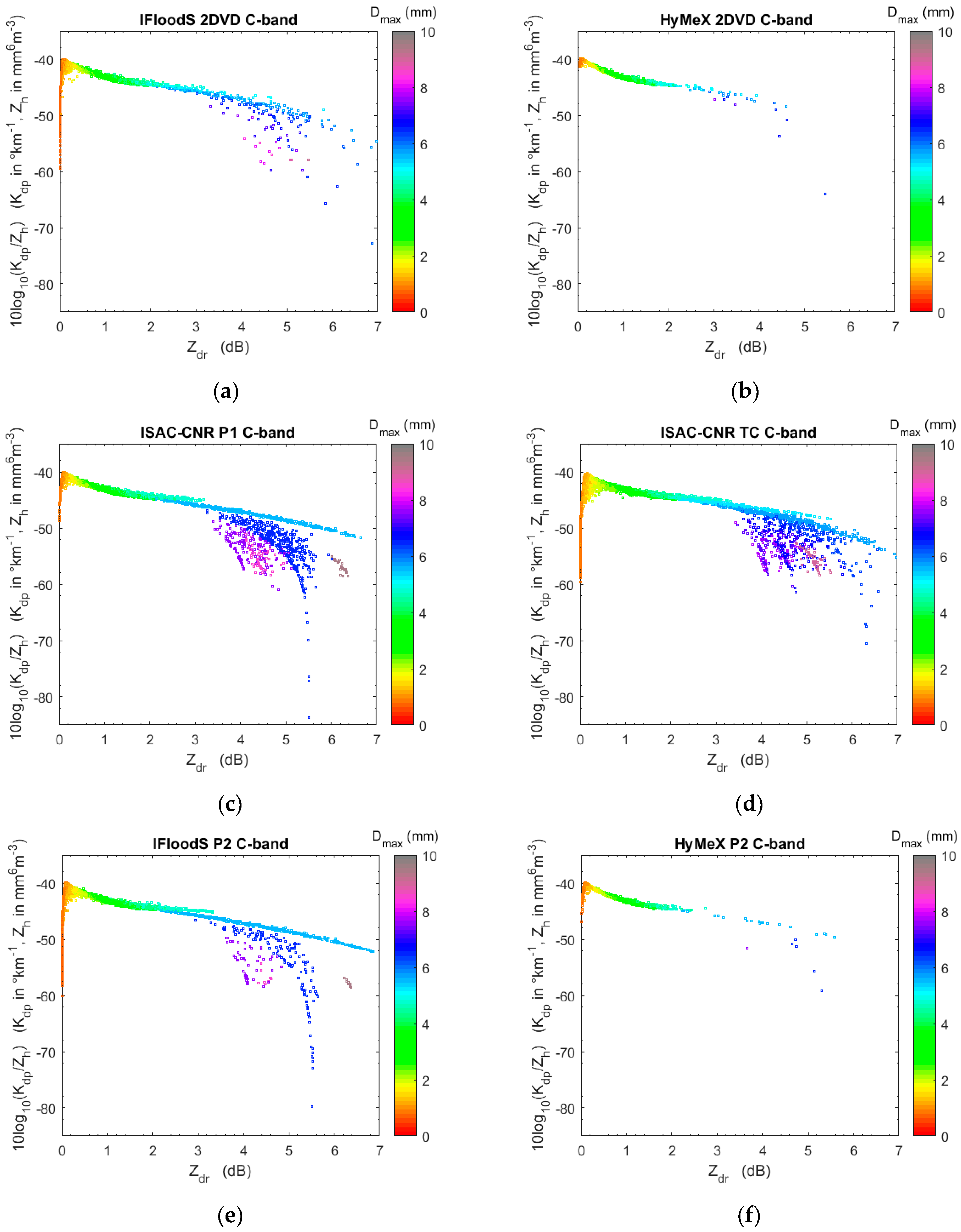
4. Sensitivity of Weather Radar Algorithms to Disdrometer Type

The studies mentioned above show that different types of co-located disdrometers provide DSDs that differ in particular in the upper and lower part of the distribution (namely small and large drops). Such differences have an impact on the variables estimated from Equations (4)–(7) and on the coefficients of the algorithms (8)–(13). The disagreement in shapes of measured DSD among different types of disdrometers can impact the various rainfall parameters differently: an overestimation of the number of large drops has a higher effect on the radar reflectivity factor, which in the Rayleigh-Gans scattering regime is the sixth moment of the DSD, than on the rainfall rate, which is roughly the third moment of the DSD. Consequently, differences can arise in the weather radar algorithms obtained from DSDs collected by different types of disdrometers. In this section, we try to assess this effect by comparing the estimators (8)–(13) derived from DSDs measured by different disdrometer types deployed in the same geographic area and operated in the same time period (see Section 2.1).

For each of the nine datasets considered in the study (see Table 1), the estimated weather radar algorithms (8)–(13) were obtained following both the 1-min DRM and the SIFT approach. Figure 7 shows the algorithms obtained with the SIFT approach for the three frequencies. In particular, Figure 7l–n shows the R estimates obtained for a given range of Z_h and for the Z_dr values that correspond to the best power-law fit between Z_h and Z_dr (namely, $Z_h=c_1{Z_{dr}}^{c_2}$; [48]). The coefficients of the Z_h(Z_dr) estimator were obtained using experimental DSD measured by TC and are c₁ = 0.1090 and c₂ = 0.2785 for S-band, c₁ = 0.0932 and c₂ = 0.3066 for C-band, and c₁ = 0.1438 and c₂ = 0.2584 for X-band. The authors would like to underline that in this study, the Z_h(Z_dr) estimator was used for plotting and comparing purposes. Similarly, in Figure 7r–t the best power-law fit $Z_{dr}=c_3{K_{dp}}^{c_4}$ is used (c₃ = 3.0597 and c₄ = 0.4069 at S-band, c₃ = 2.7088 and c₄ = 0.4714 at C-band and c₃ = 0.2715 and c₄ = 0.4385 at X-band) to obtain the rainfall rate. Furthermore, for each algorithm, the corresponding statistical parameters (14) and (15) are shown in Figure 8. Please note that we do not show coefficients of all the estimators derived from the different datasets for the sake of brevity, but also because some parameterizations do not have climatological validity since they are based on only two months of data; however, they are useful for evaluating the effects of the different disdrometer types.

Figure 7 and Figure 8 provide an overview of all estimators (8)–(13) obtained from the different types of disdrometer and, as a first step, make it possible to qualitatively evaluate the effect of the disdrometer type on the algorithms. Generally speaking, looking at Figure 7 and Figure 8, we can assert that the coefficients and the parameterization errors of the relations (8)–(13) derived from DSD datasets collected by different disdrometers are similar, indicating a moderate influences of the type of disdrometer on the relations (8)–(13). The attenuation retrieval algorithms are very similar at S-band (Figure 7a,d), while higher differences are evident at C-band (Figure 7b,c). R(K_dp,Z_dr) seems to be the algorithm least sensitive to disdrometer type; in fact, the different lines in Figure 7r–t are very close, indicating that different disdrometers provide similar algorithm-based R estimates for given values of K_dp. On the other hand, more differences in the R estimates are obtained when R(K_dp) algorithms derived from different sets of disdrometer data are used (Figure 7o–q). For R(Z_h) and R(Z_h,Z_dr), some differences are evident for values of Z_h > 45 dB (Figure 7g–i,l–n). From Figure 8, we can conclude that a small reduction of the parameterization errors (namely NMAE, NB) between DSD-based parameters and estimated parameters is evident for the weather radar algorithms obtained from 2DVD datasets with respect to those obtained from the optical disdrometer dataset. A similar conclusion can be drawn for the 1-min DRM approach (not shown for brevity) and for the other two merit factors considered in this study (RMSE and cc).

To quantify the effect of disdrometer type on the relations (8)–(13), the disdrometer-based radar algorithms derived from the different measured DSD datasets were compared in pairs. In other words, for a given radar relation, the difference in terms of weather radar algorithms obtained from a different type of disdrometer is defined as the NMAE between the estimates obtained from two different DSD datasets. To obtain these NMAE values, the nine available datasets were compared as follow: ISAC-CNR P1 vs. ISAC-CNR TC, ISAC-CNR P1_sub vs. ISAC-CNR TC_sub, ISAC-CNR TC_HY vs. HyMeX P2, HyMeX P2 vs. HyMeX 2DVD and IFloodS P2 vs. IFloodS 2DVD.

Table 4. For each frequency, the values of NMAE (in %) obtained by pairwise comparison of the parameters estimated through the weather radar algorithm established from 1-min DSDs collected by the different devices are reported, as described in the title of each column of the table. The values in brackets refer to the NMAE obtained using the SIFT approach.

S-Band
	ISAC-CNR P1 vs. ISAC-CNR TC	ISAC-CNR P1sub vs. ISAC-CNR TCsub	ISAC-CNR TCHy vs. HyMeX P2	HyMeX 2DVD vs. HyMeX P2	IFloodS 2DVD vs. IFloodS P2
ah = α1 Kdp	5% (3%)	2% (2%)	5% (7%)	15% (3%)	14% (2%)
ad = α2 Kdp	11% (5%)	8% (18%)	1% (5%)	109% (69%)	84% (31%)
R = α3 Zhβ3	2% (5%)	8% (11%)	15% (10%)	14% (12%)	19% (14%)
R = α4 Zhβ4Zdrγ4	6% (5%)	10% (4%)	3% (3%)	17% (16%)	10% (2%)
R = α5 Kdp	5% (6%)	6% (5%)	9% (6%)	19% (18%)	13% (10%)
R = α6 Zdrβ6Kdpγ6	5% (3%)	9% (2%)	1% (3%)	7% (13%)	6% (2%)
C-Band
	ISAC-CNR P1 vs. ISAC-CNR TC	ISAC-CNR P1sub vs. ISAC-CNR TCsub	ISAC-CNR TCHy vs. HyMeX P2	HyMeX 2DVD vs. HyMeX P2	IFloodS 2DVD vs. IFloodS P2
ah = α1 Kdp	2% (3%)	9% (14%)	0% (10%)	19% (11%)	21% (21%)
ad = α2 Kdp	9% (11%)	6% (14%)	6% (10%)	34% (22%)	34% (34%)
R = α3 Zhβ3	6% (3%)	15% (22%)	28% (24%)	28% (32%)	29% (33%)
R = α4Zhβ4Zdrγ4	4% (2%)	10% (20%)	13% (9%)	16% (17%)	6% (32%)
R = α5 Kdp	9% (10%)	2% (0%)	12% (10%)	14% (16%)	7% (8%)
R = α6 Zdrβ6Kdpγ6	5% (5%)	2% (1%)	1% (16%)	6% (4%)	5% (5%)
X-Band
	ISAC-CNR P1 vs. ISAC-CNR TC	ISAC-CNR P1sub vs. ISAC-CNR TCsub	ISAC-CNR TCHy vs. HyMeX P2	HyMeX 2DVD vs. HyMeX P2	IFloodS 2DVD vs. IFloodS P2
ah = α1 Kdp	4% (4%)	3% (4%)	7% (5%)	5% (8%)	1% (1%)
ad = α2 Kdp	0% (1%)	7% (8%)	6% (2%)	15% (19%)	8% (8%)
R = α3 Zhβ3	2% (6%)	8% (10%)	18% (12%)	9% (13%)	18% (19%)
R = α4 Zhβ4Zdrγ4	10% (14%)	13% (8%)	3% (44%)	7% (42%)	6% (23%)
R = α5 Kdp	5% (5%)	5% (4%)	6% (5%)	10% (11%)	6% (6%)
R = α6 Zdrβ6Kdpγ6	4% (4%)	5% (1%)	2% (5%)	8% (5%)	2% (2%)

shows, for each estimator and for each frequency, the values of NMAE obtained through pairwise comparison of the estimates obtained from weather radar algorithms based on 1-min measured DSDs and following the SIFT approach (values in brackets). Therefore, in this case, the x and y values of (15) are estimates (i.e., R and a_h, a_d from Equations (8)–(13)) derived from two different disdrometer datasets. Lower is the values of NMAE and better is the agreement between the estimator (8)–(13), or in other words, lower is the influence of the disdrometer type on the weather radar algorithm. Table 4 shows that the errors in terms of mean NMAE obtained when comparing the attenuation at horizontal polarization estimated from relations derived from DSD collected by different laser disdrometers (despite being from different manufacturers or of different versions) are limited (less than 5%). When the 2DVD-based horizontal attenuation estimators are compared with those obtained from P2 DSDs, the errors increase, reaching 15% at S-band and 21% at C-band for both the considered 2DVD-P2 pairs (namely, the ones installed in Rome during HyMeX and the ones installed in Iowa during IFloodS). Meanwhile, at X-band, the errors remain low when 2DVD and P2 results are compared. Therefore, we can conclude that estimator (8) is influenced by the type of device used to establish the relation at S- and C-band, while the effect at X-band is limited. As shown in Figure 5, at C-band, the resonance effects on the big drops is higher with respect to X- and S-band; therefore, the possible difference on the sampling of large drops among different devices has a higher impact on the obtained estimators. The effect of the SIFT approach is limited, and it does not have a clear trend. In fact, sometimes, it reduces the differences between the devices and sometimes it increases them. Similar conclusions can also be drawn for the differential attenuation estimators (9). In fact, also in this case, the differences between the estimated attenuations are higher when 2DVD and P2-based relations are compared at S- and C-band, while lower NMAE values are obtained when comparing different types of laser disdrometers. For the X-band, the discrepancy between 2DVD and P2 datasets is smoothed obtaining an error lower than 15%. It should be noted that the remarkable differences for differential attenuation at S-band are due to the limited range of these values.

Reflectivity-based rain rate estimators (10) derived from the ISAC-CNR P1 and ISAC-CNR TC datasets show negligible differences, with a discrepancy in terms of rain rate lower that 6% for all three bands. The latter error increases for all three bands when P2 vs. TC and 2DVD vs. P2-based relations are compared, the highest values of NMAE being obtained for the C-band (Table 4). These results underscore the fact that disdrometers with different measurement principles provide R(Z_h) estimates that can differ by up to 30% in mean, although the devices are co-located and reasonably sample the same precipitation. A slight increase of the NMAE values in Table 4 is observed when the two subsets, ISAC-CNR P1_sub and ISAC-CNR TC_sub are compared, indicating the likely influence of the type of precipitation on the results. Please note that the use of the SIFT approach does not produce a systematic reduction of the discrepancies between the reflectivity-based rain rate derived from different DSD datasets. However, as also shown in Figure 8g–i, the discrepancy among the R-Z_h estimators derived from different disdrometer types is higher for very low and very high values of horizontal reflectivity. In fact, the same errors in the range from 15 dB to 35 dB (which correspond roughly to the 15th and 90th percentile of the horizontal reflectivity values computed for the ISAC-CNR TC dataset) decrease, resulting in mean differences less than 10% in terms of estimated rain rate in most of the cases. Limiting Z_h between 15 dB and 35 dB means considering precipitation that varies roughly between 0.3 mm h⁻¹ and 5 mm h⁻¹.

For polarimetric rain rate estimators (11)–(13), the obtained NMAE values (Table 4) are, in general, lower than (or comparable to) those obtained for the R(Z_h) relation, indicating that they are less sensitive to the disdrometer type that collected the experimental DSDs. The latter consideration is particularly valid for the C-band. In fact, for the C-band frequency, the NMAE values between polarimetric-based rainfall estimates from 2DVD and P2 datasets is considerably lower (values lower than 15%) than that obtained comparing the 2DVD vs. P2 R(Z_h) estimates (roughly 30%). This result can be explained by considering that polarimetric rain rate estimators are usually less sensitive to DSD variability. The R(K_dp,Z_dr) estimator is the least sensitive to the disdrometer type; in fact, the NMAE values are less than 10% for each considered pair of datasets and for each frequency.

Finally, we evaluate the differences among the polarimetric rain rate estimators for different rain types, namely, light (i.e., R < 2.5 mm h⁻¹), moderate (2.5 mm h⁻¹ < R < 10 mm h⁻¹) and heavy (R > 10 mm h⁻¹). In general, the lowest differences among R(Z_h,Z_dr) relations derived from different datasets are obtained for moderate rain with values of NMAE very low and always lower than 10%. For R(K_dp) there are no differences with rain type, since it is a linear estimator. Finally, the differences for R(K_dp,Z_dr) as a function of the rain type are less pronounced.

5. Weather Radar Algorithms for Italian Climatology

Two of the datasets considered in this study (namely, ISAC-CNR P1 and ISAC-CNR TC) are the longest DSD time series so far collected in Rome (Italy) and, taking into account the possible differences with respect to other disdrometer types, as shown in the previous section, they can be used to establish weather radar algorithms optimized for Italian climatology classified as Csa (C: hot temperature, s: summer dry, a: hot summer) in [49]. We found that the differences in terms of weather radar algorithms between the different types of optical disdrometers are limited, in particular when Parsivel and ThiesClima are compared. Furthermore, in Section 3 we evaluated the advantages of the SIFT approach in reducing spurious DSD variability within a measured dataset.

Table 5. Coefficients of the estimators (9)–(14) obtained from ISAC-CNR TC dataset for S-, C- and X-bands along with the values of the NMAE (in %), NB (in %), corr and RMSE (in dB km⁻¹ or mm h⁻¹).

ISAC-CNR TC—S-Band—SIFT Approach
	α	β	γ	NMAE	NB	Corr	RMSE
ah = α1 Kdp	0.0134	\	\	26%	−22%	0.988	0.0004
ad = α2 Kdp	0.0041	\	\	47%	18%	0.918	0.0003
R = α3 Zhβ3	0.0224	0.6354	\	15%	−2%	0.983	1.05
R = α4 Zhβ4Zdrγ4	0.0040	0.9461	−3.5300	14%	−8%	0.994	0.66
R = α5 Kdp	33.6200	\	\	37%	−33%	0.980	1.45
R = α6 Zdrβ6Kdpγ6	87.5898	−1.8417	0.9580	8%	−4%	0.998	0.33
ISAC-CNR TC—C-Band—SIFT Approach
	α	β	γ	NMAE	NB	corr	RMSE
ah = α1 Kdp	0.1154	\	\	29%	20%	0.983	0.0082
ad = α2 Kdp	0.0404	\	\	67%	52%	0.966	0.0043
R = α3 Zhβ3	0.0510	0.5397	\	25%	2%	0.937	1.99
R = α4 Zhβ4Zdrγ4	0.0778	0.4705	0.5587	28%	4%	0.938	1.96
R = α5 Kdp	16.1810	\	\	37%	−33%	0.981	1.41
R = α6 Zdrβ6Kdpγ6	24.0739	−0.3855	0.8383	8%	−4%	0.997	0.45
ISAC-CNR TC—X-Band—SIFT Approach
	α	β	γ	NMAE	NB	corr	RMSE
ah = α1 Kdp	0.3454	\	\	15%	12%	0.997	0.0144
ad = α2 Kdp	0.0649	\	\	35%	27%	0.990	0.0054
R = α3 Zhβ3	0.0342	0.5662	\	18%	−3%	0.976	1.22
R = α4Zhβ4Zdrγ4	0.0089	0.8524	−3.5254	18%	−6%	0.985	0.97
R = α5 Kdp	11.3739	\	\	31%	−28%	0.988	1.16
R = α6 Zdrβ6Kdpγ6	23.4934	−1.1082	0.9325	6%	−3%	0.999	0.29

reports the values of the coefficients of the estimators (8)–(13) derived from the ISAC-CNR TC dataset. The estimators were defined using the SIFT approach with M = 10. To the best of our knowledge, the relations reported in Table 5 represent the first attempt to provide weather radar algorithms optimized for Italian climatology based on a very long time series of quality control measured DSDs. Furthermore, for each relation, the merit parameters were reported (namely (14)–(17)) in order to give a suggestion of the quality of the fit and therefore of the intrinsic error related to the provided relations.

Of the two attenuation estimators (8) and (9), a_h(K_dp) is the one with the lowest error for all the three bands; the lowest value of NMAE (i.e., 15%) is obtained for the X-band, indicating that the scatter of the data along the best fit line is the smallest. However, as expected, the error in terms of RMSE (in dB km⁻¹) is higher for the X-band (0.0144 dB km⁻¹) than for the S- and C-bands due to the fact that the attenuation effects are more pronounced at higher frequencies. Among the rainfall rate estimators (10)–(13), the R(K_dp,Z_dr) fit is that with the highest accuracy (NMAE less than 8%, RMSE less than 0.45 mm h⁻¹ and negligible bias for all bands). Comparable values of the merit parameters are obtained for R(Z_h) and R(Z_h,Z_dr) estimators in terms of NMAE and NB, although a slightly higher RMSE is associated with the reflectivity-rainfall rate estimator. Low values of NB for the R(Z_h) estimator are obtained; at C-band, the use of the SIFT approach decreases the bias considerably (NB for R(Z_h) with the 1-min DRM approach is 16%), while for the S- and X-bands, the reduction is smaller. Finally, the R(K_dp) estimator is the one with the highest values of NMAE, NB and RMSE. The biases associated with the R(K_dp) estimator are negative for all the considered frequencies, indicating an underestimation of the rainfall rate derived from the algorithm with respect to that obtained directly from the measured DSDs. The high values of NB for the R(K_dp) estimator indicate the poor performance of this algorithm in comparison to the other rainfall estimators. The latter’s errors are higher at S-, and C-band with respect to X-band.

To provide weather radar algorithms that are more accurate for different rain types,

Table 6. As for Table 5, but for convective rain.

ISAC-CNR TC—S-Band—SIFT Approach—Convective Rain
	α	β	γ	NMAE	NB	Corr	RMSE
ah = α1 Kdp	0.0130	\	\	9%	−3%	0.977	0.0013
ad = α2 Kdp	0.0042	\	\	31%	−1%	0.842	0.0013
R = α3 Zhβ3	0.0046	0.7688	\	16%	0%	0.955	4.33
R = α4 Zhβ4Zdrγ4	0.0012	1.0712	−3.9424	5%	0%	0.993	1.41
R = α5 Kdp	31.779	\	\	12%	−5%	0.982	3.14
R = α6 Zdrβ6Kdpγ6	90.606	−1.9383	1.0313	3%	0%	0.996	0.78
ISAC-CNR TC—C-Band—SIFT Approach—Convective Rain
	α	β	γ	NMAE	NB	Corr	RMSE
ah = α1Kdp	0.1180	\	\	16%	6%	0.976	0.0317
ad = α2 Kdp	0.0422	\	\	23%	10%	0.968	0.0151
R = α3 Zhβ3	0.0223	0.6083	\	30%	−1%	0.824	8.47
R = α4Zhβ4Zdrγ4	0.0163	0.6552	−0.3297	29%	−1%	0.825	8.44
R = α5 Kdp	15.2837	\	\	11%	−5%	0.987	2.84
R = α6 Zdrβ6Kdpγ6	23.3346	−0.4995	0.9521	6%	0%	0.992	1.49
ISAC-CNR TC—X-Band—SIFT Approach—Convective rain
	α	β	γ	NMAE	NB	Corr	RMSE
ah = α1 Kdp	0.3526	\	\	4%	2%	0.995	0.0376
ad = α2 Kdp	0.0672	\	\	10%	2%	0.984	0.0169
R = α3 Zhβ3	0.0058	0.7091	\	18%	−1%	0.943	4.90
R = α4 Zhβ4Zdrγ4	0.0033	0.9806	−4.4888	10%	0%	0.980	2.76
R = α5 Kdp	10.7913	\	\	8%	−4%	0.990	2.24
R = α6 Zdrβ6Kdpγ6	22.0551	−1.1018	0.9754	3%	0%	0.995	1.00

and

Table 7. As for Table 5, but for stratiform rain.

ISAC-CNR TC—S-Band—SIFT Approach—Stratiform Rain
	α	β	γ	NMAE	NB	Corr	RMSE
ah = α1 Kdp	0.0201	\	\	21%	−15%	0.982	0.0001
ad = α2 Kdp	0.0032	\	\	53%	32%	0.669	0.0001
R = α3 Zhβ3	0.0246	0.6390	\	15%	2%	0.968	0.48
R = α4 Zhβ4Zdrγ4	0.0066	0.9678	−5.6907	7%	−1%	0.993	0.22
R = α5 Kdp	64.9792	\	\	20%	−16%	0.982	0.45
R = α6 Zdrβ6Kdpγ6	101.9187	−2.3339	0.9420	6%	−2%	0.997	0.14
ISAC-CNR TC—C-Band—SIFT Approach—Stratiform Rain
	α	β	γ	NMAE	NB	Corr	RMSE
ah = α1 Kdp	0.0729	\	\	14%	−4%	0.978	0.0010
ad = α2 Kdp	0.0120	\	\	50%	23%	0.859	0.0005
R = α3 Zhβ3	0.0867	0.4749	\	31%	10%	0.913	0.80
R = α4 Zhβ4Zdrγ4	0.0510	0.6257	−2.7690	27%	9%	0.927	0.74
R = α5 Kdp	31.6234	\	\	20%	−15%	0.987	0.40
R = α6Zdrβ6Kdpγ6	30.9720	−0.7932	0.8653	8%	−2%	0.994	0.21
ISAC-CNR TC—X-Band—SIFT Approach—Stratiform Rain
	α	β	γ	NMAE	NB	Corr	RMSE
ah = α1 Kdp	0.2615	\	\	7%	1%	0.995	0.0026
ad = α2 Kdp	0.0365	\	\	26%	15%	0.953	0.0013
R = α3 Zhβ3	0.0461	0.5480	\	21%	4%	0.948	0.61
R = α4 Zhβ4Zdrγ4	0.0128	0.8740	−4.8960	13%	1%	0.971	0.45
R = α5 Kdp	19.1441	\	\	18%	−13%	0.992	0.33
R = α6Zdrβ6Kdpγ6	23.6538	−1.0178	0.9194	7%	−2%	0.997	0.15

report the estimators (8)–(13) obtained at different frequencies from convective DSD samples and stratiform DSD samples of the ISAC-CNR TC dataset, respectively. Considering the attenuation estimators, the performance of the fitting in terms of NMAE is better for convective rain than for stratiform rain. This is due to the fact that K_dp at low rain intensity can be very low, and therefore the dispersion of the data along the best fit relation is higher for stratiform rain. On the other hand, a higher value of RMSE is obtained for convective attenuation estimators with respect to the stratiform one because the attenuation increases, increasing the precipitation intensity. The coefficients of the attenuation estimators for all rain and convective rain are very close, while those obtained for stratiform rain are lower. Similar considerations are valid for R(K_dp) estimators.

The performance of the fitting for R(Z_h) estimators does not change considerably between all rain, convective rain and stratiform rain; however, some differences are evident in the values of the relation coefficients. At S- and X-bands, the prefactor α₃ for convective rain is one order of magnitude less than that obtained for all rain and stratiform rain. Meanwhile, at C-band, the prefactors for the different rain types are more similar.

6. Conclusions

As widely reported in the literature, co-located disdrometers can sample the DSD differently due to the differences in hardware and software. The main discrepancies between the devices are in the lower and upper parts of the spectra (namely, small and large drops) and in the number of detected drops. These disagreements produce differences in the integral rainfall parameters estimated from measured DSD, and the impact of the DSD disagreement varies from one parameter to another, despite the fact that disdrometer measurements are often considered to be “ground truth” and are used to establish weather radar algorithms applied to retrieve rainfall rate or attenuation from remote sensing measurements.

In this study, a huge amount of DSDs collected by different types of disdrometers were used (i) to establish weather radar algorithms at S-, C- and X-band considering two different techniques, and (ii) to evaluate the impact of the instrumental errors on these algorithms. In particular, the weather radar algorithms were established from (i) 1-min samples, and (ii) following the SIFT approach. Comparing the two techniques, we found that:

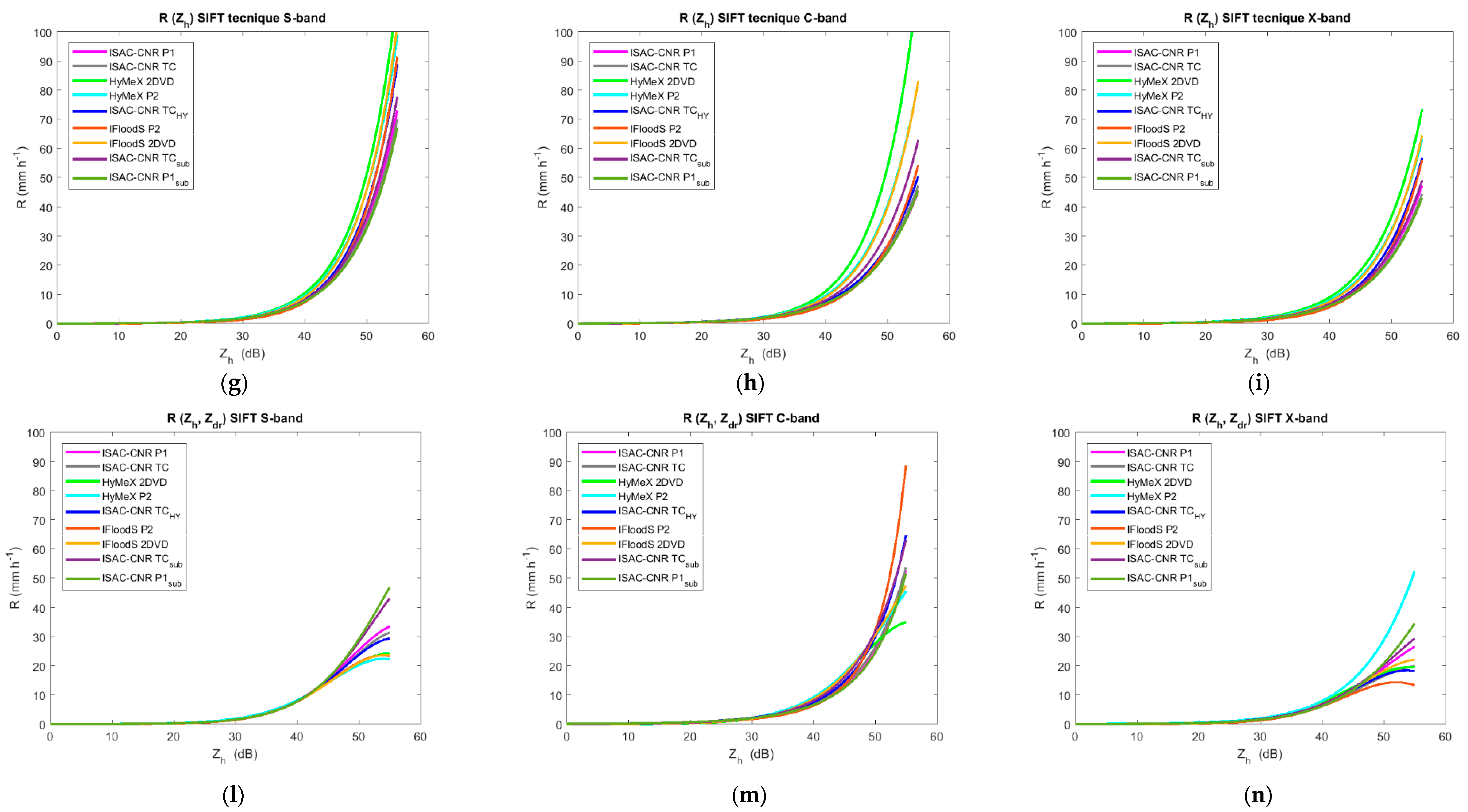
• as also demonstrated in [17], we confirm that the use of the SIFT approach to establish the R-Z_h relation from measured DSDs makes it possible to reduce the intrinsic error of the parameterization, or, in other words, to provide a more stable relation. We found, for all three bands, a reduction in the NMAE of between 50% and 60% when the SIFT approach was used;
• testing the effect of the SIFT approach on all the other weather radar algorithms considered in this study, we found that the specific attenuation estimators (i.e., Equations (8) and (9)) and the polarimetric rainfall rate estimators (i.e., Equations (11)–(13)) also benefit from the application of SIFT. A reduction of NMAE of between 10% and 50% was obtained for these estimators, with a few exceptions for the R(Z_h,Z_dr) relation at C- and X-band;
• the reduction of the NMAE due to the application of the SIFT approach is independent of the type of disdrometer used to collect the data.

Regarding the effect of the disdrometer type on the weather radar algorithm estimations, we can summarize the main results as follows:

• the SIFT approach does not have a clear and unequivocal effect on the comparison between weather radar algorithm obtained from different disdrometer types. In other words, although SIFT reduces the scatter of the data along the best fit relation, it conserves the differences among the devices; in fact, the disagreement obtained when comparing different devices, although limited, is not always reduced when the SIFT approach is adopted instead of the 1-min DRM;
• the coefficients of the relations for rain rate and specific attenuation estimation in Equations (8)–(13) derived from different DSD datasets are similar; also, the parameterization errors are comparable;
• the comparison of radar algorithms obtained from different types of laser disdrometers (namely P1, P2 or TC) gives an error of less than 10% for all (except for very few exceptions) of the considered relations and frequencies;
• the agreement in terms of radar algorithm estimates between P2 and 2DVD (which is considered the most accurate commercial disdrometer for measurements of DSD) is a bit lower, in particular at S- and C-band, with differences in rainfall rate (differential attenuation) estimates that can reach 30% at C-band when the R(Z_h) (a_d(K_dp)) estimator is considered;
• limiting the comparison to moderate rainfall (2.5 mm h⁻¹ < R < 10 mm h⁻¹), the disagreement between 2DVD and P2 estimates R(Z_h) and R(Z_dr, K_dp) decreases (maximum values 10%);
• it is confirmed that polarimetric rain rate estimators seem to be less sensitive to disdrometer type with respect to the R(Z_h) relation, in particular at C-band.

Taking into account the results obtained in this study and the characteristics of the disdrometer-measured dataset used (see Table 1) we can conclude that the use of a low-cost easy-maintenance laser disdrometer to establish long-term climatological radar algorithms does not produce considerable differences in comparison to more accurate devices such as the 2DVD, whereas for single events, a more accurate microphysical analysis can benefit from the use of more sophisticated 2DVD.

Finally, for the first time, we provided radar algorithms optimized for Italian climatology based on a long time series of measured DSDs in Rome. The use of this relation is expected to improve the QPE estimation from radar systems in Italy.

References

1. Marshall, J.S.; Palmer, W.M. The distribution of raindrops with size. J. Meteorol. 1948, 9, 327–332. [Google Scholar] [CrossRef]
2. Bringi, V.N.; Chandrasekar, V. Polarimetric Doppler Weather Radar Principles and Applications; Cambridge University Press: Cambridge, UK, 2001; p. 648. ISBN 0-521-62384-7. [Google Scholar]
3. Tapiador, F.J.; Checa, R.; De Castro, M. An experiment to measure the spatial variability of rain drop size distribution using sixteen laser disdrometers. Geophys. Res. Lett. 2010, 37, L16803. [Google Scholar] [CrossRef]
4. Battan, L.J. Radar Observation of the Atmosphere; University of Chicago Press: Chicago, IL, USA, 1973; ISBN 9780226039190. [Google Scholar]
5. Gorgucci, E.; Scarchilli, G.; Chandrasekar, V.; Bringi, V.N. Rainfall estimation from polarimetric radar measurements: Composite algorithms immune to variability in raindrop shape–size relation. J. Atmos. Ocean. Technol. 2001, 18, 1773–1786. [Google Scholar] [CrossRef]
6. Bringi, V.N.; Chandrasekar, V.; Balakrishnan, N.; Zrnić, D.S. An Examination of Propagation Effects in Rainfall on Radar Measurements at Microwave Frequencies. J. Atmos. Ocean. Technol. 1990, 7, 829–840. [Google Scholar] [CrossRef] [Green Version]
7. Tokay, A.; Kruger, A.; Krajewski, W. Comparison of drop-size distribution measurements by impact and optical disdrometers. J. Appl. Meteorol. 2001, 40, 2083–2097. [Google Scholar] [CrossRef]
8. Adirosi, E.; Gorgucci, E.; Baldini, L.; Tokay, A. Evaluation of gamma raindrop size distribution assumption through comparison of rain rates of measured and radar-equivalent gamma DSD. J. Appl. Meteorol. Climatol. 2014, 53, 1618–1635. [Google Scholar] [CrossRef]
9. Adirosi, E.; Baldini, L.; Lombardo, F.; Russo, F.; Napolitano, F.; Volpi, E.; Tokay, A. Comparison of different fittings of drop spectra for rainfall retrievals. Adv. Water Resour. 2015, 83, 55–67. [Google Scholar] [CrossRef]
10. Adirosi, E.; Volpi, E.; Lombardo, F.; Baldini, L. Raindrop size distribution: Fitting performance of common theoretical models. Adv. Water Resour. 2016, 96, 290–305. [Google Scholar] [CrossRef]
11. Johnson, R.W.; Kliche, D.V.; Smith, P.L. Comparison of estimators for parameters of gamma distributions with left-truncated samples. J. Appl. Meteorol. Climatol. 2011, 50, 296–310. [Google Scholar] [CrossRef]
12. Chandrasekar, V.; Bringi, V.N.; Balakrishnan, N.; Zrnic, D.S. Error structure of multiparameter radar and surface measurements of rainfall. Part III: Specific differential phase. J. Atmos. Ocean. Technol. 1990, 7, 621–629. [Google Scholar] [CrossRef]
13. Smith, P.L.; Liu, Z.; Joss, J. A study of sampling-variability effects in raindrop size observations. J. Appl. Meteorol. 1993, 32, 1259–1269. [Google Scholar] [CrossRef]
14. Smith, P.L. Sampling issues in estimating radar variables from disdrometer data. J. Atmos. Ocean. Technol. 2016, 33, 2305–2313. [Google Scholar] [CrossRef]
15. Gorgucci, E.; Baldini, L. An examination of the validity of the mean raindrop-shape model for dual-polarization radar rainfall retrievals. IEEE Geosci. Remote Sens. 2009, 47, 2752–2761. [Google Scholar] [CrossRef]
16. Tapiador, F.J.; Turk, F.J.; Petersen, W.; Hou, A.Y.; Garcia-Ortega, E.; Machado, L.A.T.; Angelis, C.F.; Salio, P.; Kidd, C.; Huffman, G.J.; et al. Global precipitation measurement: Methods, datasets and applications. Atmos. Res. 2012, 104, 70–97. [Google Scholar] [CrossRef]
17. Lee, G.W.; Zawadzki, I. Variability of drop size distributions: Noise and noise filtering in disdrometric data. J. Appl. Meteorol. 2005, 44, 634–652. [Google Scholar] [CrossRef]
18. Cao, Q.; Zhang, G.; Brandes, E.; Schuur, T.; Ryzhkov, A.; Ikeda, K. Analysis of video disdrometer and polarimetric radar data to characterize rain microphysics in Oklahoma. J. Appl. Meteorol. Climatol. 2008, 47, 2238–2255. [Google Scholar] [CrossRef]
19. Park, S.G.; Kim, H.L.; Ham, Y.W.; Jung, S.H. Comparative evaluation of the OTT PARSIVEL2 using a collocated two-dimensional video disdrometer. J. Atmos. Ocean. Technol. 2017, 34, 2059–2082. [Google Scholar] [CrossRef]
20. Chen, H.; Chandrasekar, V.; Bechini, R. An improved dual-polarization radar rainfall algorithm (DROPS2.0): Application in NASA IFloodS field campaign. J. Hydrometeorol. 2017, 18, 917–937. [Google Scholar] [CrossRef]
21. Lanza, L.G.; Vuerich, E. Non-parametric analysis of one-minute rain intensity measurements from the WMO Field Intercomparison. Atmos. Res. 2012, 103, 52–59. [Google Scholar] [CrossRef]
22. Gertzman, H.S.; Atlas, D. Sampling errors in the measurement of rain and hail parameters. J. Geophys. Res. 1977, 82, 4955–4966. [Google Scholar] [CrossRef]
23. Wong, R.K.W.; Chidambaram, N. Gamma size distribution and stochastic sampling errors. J. Clim. Appl. Meteorol. 1985, 24, 568–579. [Google Scholar] [CrossRef]
24. Nešpor, V.; Krajewski, W.F.; Kruger, A. Wind-induced error of raindrop size distribution measurement using a two-dimensional video disdrometer. J. Atmos. Ocean. Technol. 2000, 17, 1483–1492. [Google Scholar] [CrossRef]
25. Friedrich, K.; Kalina, E.A.; Masters, F.J.; Lopez, C.R. Drop-size distributions in thunderstorms measured by optical disdrometers during VORTEX2. Mon. Weather Rev. 2013, 141, 1182–1203. [Google Scholar] [CrossRef]
26. Upton, G.; Brawn, D. An investigation of factors affecting the accuracy of thies disdrometers. In Proceedings of the Technical Conference on Instruments and Methods of Observation (TECO-2008), St. Petersburg, Russia, 27–28 November 2008. [Google Scholar]
27. Thurai, M.; Petersen, W.A.; Tokay, A.; Schultz, C.; Gatlin, P. Drop size distribution comparisons between Parsivel and 2-D video disdrometers. Adv. Geosci. 2011, 30, 3–9. [Google Scholar] [CrossRef] [Green Version]
28. Tokay, A.; Petersen, W.A.; Gatlin, P.; Wingo, M. Comparison of raindrop size distribution measurements by collocated disdrometers. J. Atmos. Ocean. Techol. 2013, 30, 1672–1690. [Google Scholar] [CrossRef]
29. Tokay, A.; Wolff, D.B.; Petersen, W.A. Evaluation of the new version of the laser-optical disdrometer, OTT Parsivel2. J. Atmos. Ocean. Techol. 2014, 31, 1276–1288. [Google Scholar] [CrossRef]
30. Ferretti, R.; Pichelli, E.; Gentile, S.; Maiello, I.; Cimini, D.; Davolio, S.; Miglietta, M.M.; Panegrossi, G.; Baldini, L.; Pasi, F.; et al. Overview of the first HyMeX special observation period over italy: Observations and model results. Hydrol. Earth Syst. Sci. 2014, 18, 1953–1977. [Google Scholar] [CrossRef] [Green Version]
31. Roberto, N.; Adirosi, E.; Baldini, L.; Casella, D.; Dietrich, S.; Gatlin, P.; Panegrossi, G.; Petracca, M.; Sanò, P.; Tokay, A. Multi-sensor analysis of convective activity in central Italy during the HyMeX SOP 1.1. Atmos. Meas. Technol. 2016, 9, 535–552. [Google Scholar] [CrossRef] [Green Version]
32. Petersen, W.; Gatlin, P. GPM Ground Validation Autonomous Parsivel Unit (APU) IFloodS [APU01, APU03, APU10]; NASA EOSDIS Global Hydrology Resource Center Distributed Active Archive Center: Huntsville, AL, USA, 2013. Available online: http://ghrc.nsstc.nasa.gov (accessed on 11 July 2016).
33. Petersen, W.; Gatlin, P. GPM Ground Validation Two-Dimensional Video Disdrometer (2DVD) IFloodS [SN25, SN36, SN38]; NASA EOSDIS Global Hydrology Resource Center Distributed Active Archive Center: Huntsville, AL, USA, 2013. Available online: http://ghrc.nsstc.nasa.gov (accessed on 11 July 2016).
34. Löffler-Mang, M.; Joss, J. An optical disdrometer for measuring size and velocity of hydrometeors. J. Atmos. Ocean. Technol. 2000, 17, 130–139. [Google Scholar] [CrossRef]
35. Lanzinger, E.; Theel, M.; Windolph, H. Rainfall amount and intensity measured by the Thies laser precipitation monitor. In Proceedings of the WMO Technical Conference on Meteorological and Environmental Instruments and Methods of Observation (TECO), Geneva, Switzerland, 4–6 December 2006. [Google Scholar]
36. Angulo-Martínez, M.; Beguería, S.; Latorre, B.; Fernández-Raga, M. Comparison of precipitation measurements by Ott Parsivel2 and Thies LPM optical disdrometers. Hydrol. Earth Syst. Sci. Discuss. 2017. [Google Scholar] [CrossRef]
37. Bernauer, F.; Hürkamp, K.; Rühm, W.; Tschiersch, J. On the consistency of 2-D video disdrometers in measuring microphysical parameters of solid precipitation. Atmos. Meas. Technol. 2015, 8, 3251–3261. [Google Scholar] [CrossRef] [Green Version]
38. Atlas, D.; Srivastava, R.C.; Sekhon, R.S. Doppler radar characteristics of precipitation at vertical incidence. Rev. Geophys. 1973, 11, 1–35. [Google Scholar] [CrossRef]
39. Marzuki, M.; Hashiguchi, H.; Yamamoto, M.K.; Mori, S.; Yamanaka, M.D. Regional variability of raindrop size distribution over Indonesia. Ann. Geophys. 2013, 31, 1941–1948. [Google Scholar] [CrossRef] [Green Version]
40. Thurai, M.; Bringi, V.N.; May, P.T. CPOL radar-derived drop size distribution statistics of stratiform and convective rain for two regimes in Darwin, Australia. J. Atmos. Ocean. Techol. 2010, 27, 932–942. [Google Scholar] [CrossRef]
41. Barber, P.W.; Yen, C. Scattering of electromagnetic waves by arbitrarily shaped dielectric bodies. Appl. Opt. 1975, 14, 2864–2872. [Google Scholar] [CrossRef] [PubMed]
42. Mishchenko, M.I.; Travis, L.D.; Mackowski, D.W. T-matrix computations of light scattering by nonspherical particles: A review. J. Quant. Spectrosc. Radiat. Transf. 1996, 55, 535–575. [Google Scholar] [CrossRef]
43. Beard, K.V.; Chuang, C. A new model for the equilibrium shape of raindrops. J. Atmos. Sci. 1987, 44, 1509–1524. [Google Scholar] [CrossRef]
44. Gorgucci, E.; Chandrasekar, V.; Baldini, L. Can a unique model describe the raindrop shape–size relation? A clue from polarimetric radar measurements. J. Atmos. Ocean. Technol. 2009, 26, 1829–1842. [Google Scholar] [CrossRef]
45. Gorgucci, E.; Chandrasekar, V.; Baldini, L. Microphysical retrievals from dual-polarization radar measurements at X band. J. Atmos. Ocean. Technol. 2008, 25, 729–741. [Google Scholar] [CrossRef]
46. Carey, L.D.; Petersen, W.A. Sensitivity of C-band polarimetric radar–based drop size estimates to maximum diameter. J. Appl. Meteorol. Climatol. 2015, 54, 1352–1371. [Google Scholar] [CrossRef]
47. Leinonen, J.; Moisseev, D.; Leskinen, M.; Petersen, W.A. A climatology of disdrometer measurements of rainfall in Finland over five years with implications for global radar observations. J. Appl. Meteorol. Climatol. 2012, 51, 392–404. [Google Scholar] [CrossRef]
48. Matrosov, S.Y.; Cifelli, R.; Neiman, P.J.; White, A.B. Radar rain-rate estimators and their variability due to rainfall type: An assessment based on hydrometeorology testbed data FROM the southeastern United States. J. Appl. Meteorol. Climatol. 2016, 55, 1345–1358. [Google Scholar] [CrossRef]
49. Kottek, M.; Grieser, J.; Beck, C.; Rudolf, B.; Rubel, F. World map of the Köppen-Geiger climate classification updated. Meteorol. Z. 2006, 15, 259–263. [Google Scholar] [CrossRef]
Figure 1. Locations of the disdrometers used in this study in Italy (a) and in Iowa (b).
Atmosphere 09 00360 g001
Figure 2. Scatterplot between the ratio Kdp/Zh as function of Zdr at S-band for the different datasets considered in this study. The colorbar indicates the values of the measured maximum drop diameter (Dmax). (a) IFloodS 2DVD dataset; (b) HyMeX 2DVD dataset; (c) ISAC-CNR P1 dataset; (d) ISAC-CNR TC sataset; (e) IFloodS P2 dataset; (f) HyMeX P2 dataset.
Atmosphere 09 00360 g002
Figure 3. As for Figure 2, but for C-band. (a) IFloodS 2DVD dataset; (b) HyMeX 2DVD dataset; (c) ISAC-CNR P1 dataset; (d) ISAC-CNR TC sataset; (e) IFloodS P2 dataset; (f) HyMeX P2 dataset.
Atmosphere 09 00360 g003
Figure 4. As for Figure 2, but for X-band. (a) IFloodS 2DVD dataset; (b) HyMeX 2DVD dataset; (c) ISAC-CNR P1 dataset; (d) ISAC-CNR TC sataset; (e) IFloodS P2 dataset; (f) HyMeX P2 dataset.
Atmosphere 09 00360 g004
Figure 5. Ratio between backscattering cross section (a) and differences between forward scattering amplitudes (b) at horizontal and vertical polarization as function of equivalent drop diameter for S-band (green line), C-band (blue line) and X-band (red line).
Atmosphere 09 00360 g005
Figure 6. Scatterplot of Z versus R as obtained from Thies Clima DSDs for the different frequencies considered in this study. Blue dots are for 1-min DRM and red dots are for the SIFT approach. The black lines represent the Z-R relation obtained from 1-min DRM and applying SIFT. (a) S-band; (b) C-band; (c) X-band.
Atmosphere 09 00360 g006
Figure 7. Representation of the weather radar algorithms obtained using different datasets of measured DSD and following the SIFT approach. (ac) are ah(Kdp) relations for S-, C-, and X-band, respectively; (df) are ad(Kdp) relations for S-, C- and X-band, respectively; (gi) are R(Zh) relations for S-, C-, and X-band, respectively; (ln) are R(Zh,Zdr) relations for S-, C-, and X-band, respectively; (oq) are R(Kdp) relations for S-, C-, and X-band, respectively; and (rt) are R(Zdr,Kdp) relations for S-, C-, and X-band, respectively.
Atmosphere 09 00360 g007aAtmosphere 09 00360 g007bAtmosphere 09 00360 g007c
Figure 8. For the different estimators considered in this study, (a,c e) represent the values of NMAE, and (b,d,f) those of NB at S-, C- and X-band following the SIFT approach.
Atmosphere 09 00360 g008