The Generation and Forecast of Extreme Winds during the Origin and Progression of the 2017 Tubbs Fire


1
National Center for Atmospheric Research, P.O. Box 3000, Boulder, CO 80301, USA
2
National Oceanic and Atmospheric Administration, National Environmental Satellite, Data, and Information Service, 5830 University Research Ct, College Park, MD 20740, USA
3
U.S.D.A. Forest Service, Geospatial Technology and Applications Center, 2222 West 2300 South, Salt Lake City, UT 84119, USA
*
Author to whom correspondence should be addressed.
Atmosphere 2018, 9(12), 462; https://doi.org/10.3390/atmos9120462
Submission received: 5 July 2018
/
Revised: 15 October 2018
/
Accepted: 20 November 2018
/
Published: 24 November 2018
(This article belongs to the Special Issue Fire and the Atmosphere)
Abstract
:On 8–9 October 2017, fourteen wildfires developed rapidly during a strong Diablo wind event in northern California including the Tubbs Fire, which travelled over 19 km in 3.25 h. Here, we applied the CAWFE® coupled numerical weather prediction-fire modeling system to investigate the airflow regime and extreme wind peaks underlying the extreme fire behavior using simulations that refine from a 10 km to a 185 m horizontal grid spacing. We found that as Diablo winds travelled south down the Sacramento Valley and fanned out southwestward over the Wine Country, their strength waxed and waned and their direction wavered, creating varying locations near fire origins where wind overrunning topography reached 30–40 m/s, along with streaks and bursts of strong winds in the lee of some topographic features and stagnation downstream of others. Despite a statically stable layer in the lowest 1.5 km, the high Froude number flow sometimes resembled a hydraulic jump. Elsewhere, the flow behaved similarly to neutrally-stratified flow over small hills, creating wind extrema that exceeded 40 m/s at the crest of some lesser hills including near the Tubbs fire ignition, but which shed bursts of high speed winds that travel downstream at approximately 5–7-min intervals. Nonetheless, simulated fire growth lagged satellite detection of fire arrival in Santa Rosa by up to 1 h, although whether the data detect fire line or spotting is ambiguous. A forecast simulation with a 370 m horizontal grid spacing produced an on-time fire line arrival in Santa Rosa, with calculations executed 4 times faster than real time on a single computer processor.
1. Introduction
On 8–9 October 2017, more than 170 wildfires ignited in the Wine Country, northern coastal ranges, and Butte and Nevada Counties to the west, north, and east of California’s northern Sacramento Valley (Figure 1). Of these, fourteen large fires grew rapidly, some joining into multi-fire complexes. Subsequent investigative reports [1,2] determined several of the large fires were started by electrical equipment, in some cases by branches being brought into contact with those. Many fires appeared and rapidly spread during local peaks of an unusually strong downslope wind event. Such multi-day events, termed Diablo winds, are a recognized meteorological feature of the region [3,4] and have been linked to erratic wildfire behavior, fatalities, and past destructive wildland–urban interface fires such as the 1991 Oakland Hills Fire [5] and the similar 1964 Wine Country fires [6]. In 2017’s event, the widespread outbreak of fires and their extremely rapid spread raise questions about the airflow regime that occurred and the underlying mechanisms leading to the extreme winds. The events hint at exceptional wind extrema, yet these lie between surface weather station network data locations. While regional elevated winds are captured in operational simulations, if there are extrema, they could be under-resolved in operational forecasts. We examined these issues using two approaches. First, we performed a retrospective research simulation with the CAWFE® (derived from Coupled Atmosphere–Wildland Fire Environment) coupled numerical weather prediction–wildland fire behavior modeling system. Second, we configured CAWFE without a priori knowledge of how the fire unfolded in order to predict the flow regime and subsequent Tubbs Fire growth, examining the predictability of the winds including their extrema and fire behavior.
2. Overview of Event Environment
Diablo winds are a San Francisco Bay meteorological phenomenon that arises from concurrent strong high pressure over the Great Basin and lower pressure offshore of San Francisco and Monterey. Similar to Santa Anas, this inland–offshore pressure gradient drives air downward in elevation and offshore. Climatologies developed from surface weather station data suggest that Diablo winds tend to occur overnight through morning in fall through spring [7,8]. They are characterized by low relative humidity and high wind speeds, but temperatures and ratio of wind gusts to mean wind speeds are similar to climatology [7], presenting a dry, potentially strong wind shaped by local topography.
The synoptic and fire environment during the October 2017 Wine Country fires are described in Reference [9]. A trough moved from the Pacific Northwest through the Great Basin on 8–9 October (Figure 2a,b) creating a regional pressure gradient generating winds first driven south down the Sacramento Valley (Figure 2c), then southwestward over the coastal and eastern Sacramento Valley mountain ranges (Figure 2d), encountering a sequence of topographic features with different spatial scales.
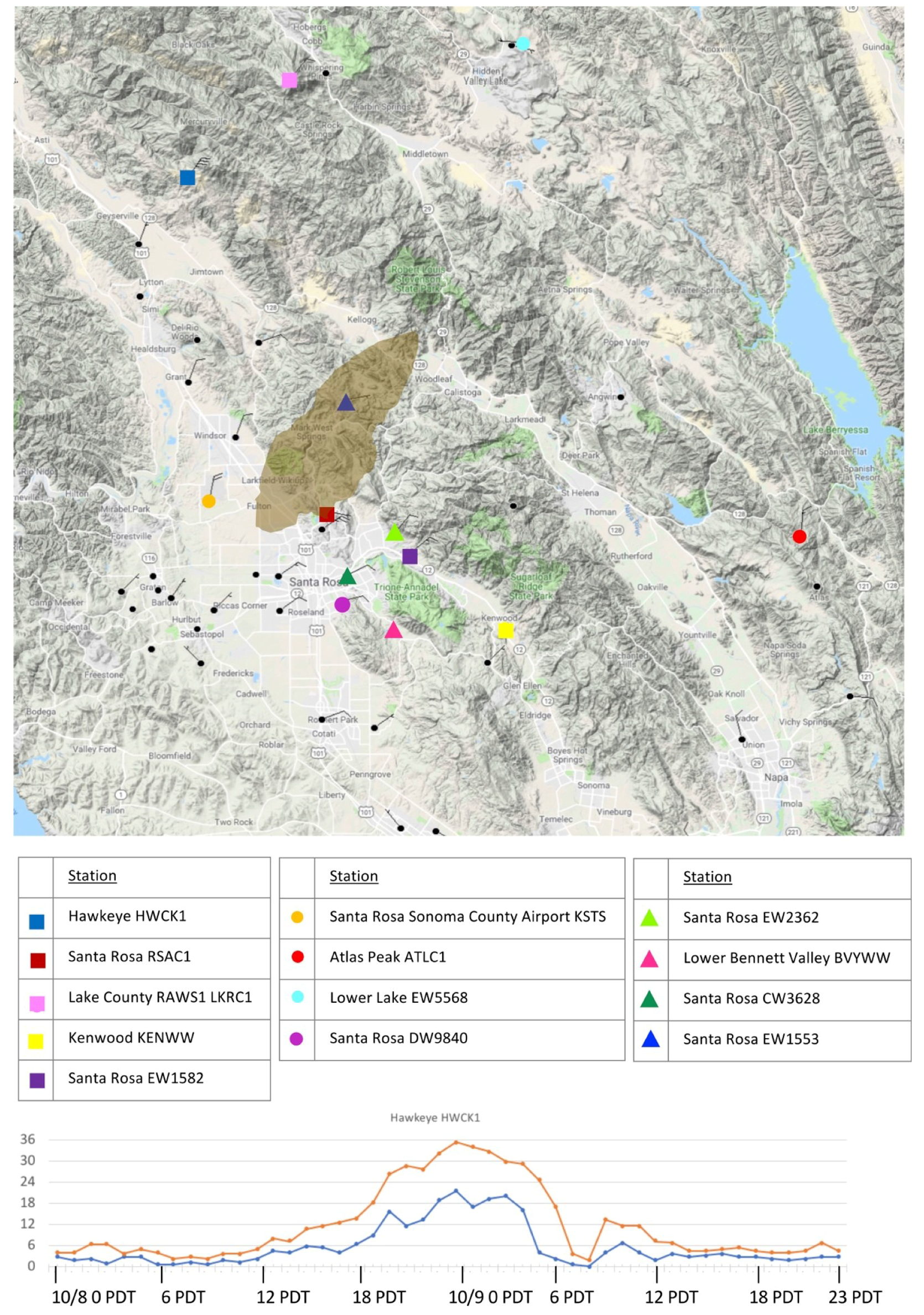
Weather station data presented a complex image of the local airflow. Several stations indicated a dramatic increase in wind speeds peaking near 12 a.m.–1 a.m. (all times Pacific Daylight Time (PDT)) on 9 October; for example, Hawkeye (HWCK1), Lake County RAWS1 (LKRC1), and Kenwood (KENWW) produced wind gusts of 36, 22, and 20 m/s, respectively, while others showed a more gradual increase beginning about 8 p.m. on 8 October. While some higher wind speeds and gusts were located on higher elevation stations (Figure 3, Figure 4 and Figure 5) (e.g., HWCK1 and LKRC1), not all nearby mountain stations recorded high winds (e.g., ATLC1). In addition, some of the highest wind speeds and gusts were located at RSAC1, on a low hill just above the valley floor, while nearby valley stations at similar positions (EW2362, EW1582, and KENWW) in the lee of a mountain ridge recorded different strengths. Gusts, the peak wind measured in the mean wind sampling period, were approximately twice the mean wind speed. These characteristics suggested speeds varied not only with elevation but with distance along the range, with locations where high winds extended out onto the Santa Rosa valley floor. The strength of both mean and gust winds experienced pulses; determination of the frequency is difficult due to the differing reporting frequency of stations.
Late on 8 October, over a dozen electrical safety incidents were reported in Wine Country, northern coastal ranges, and Butte and Nevada Counties [10]. While the cause is still under investigation, reports placed the Tubbs fire source ignition at 38.60895° N and 122.62879° W at 9:45 p.m. (http://cdfdata.fire.ca.gov/incidents/incidents_details_info?incident_id=1867) (Figure 6). Centroids of satellite-borne Moderate Resolution Imaging Spectroradiometer (MODIS) 1 km resolution active fire detections at 11:24–11:27 p.m. filled the area up to 6.7 km from the ignition location, with additional detections located up to 8.5 km away, perhaps detecting embers that may or may not have ignited additional fires. Nearly coincident data from the 375 m resolution S-NPP/VIIRS instrument at 3:09 a.m. and later MODIS observations at 3:35 a.m. showed the leading edge of fire detections had extended past Highway 101 in Fulton, California, 17.6 km from ignition, suggesting that, if the front did not already slow, the leading edge of the fire spread at an average rate of 3.0 km/h over 5.8 h. The VIIRS 3:09 A.M. observation is the only sub-kilometer resolution mapping data of the fire until its next observation at 2:53 p.m. on 9 October.
Atmospheric airflow regimes are shaped by factors including the wind speed above topographic features, atmospheric static stability, and the feature aspect ratio (height divided by half-width) of terrain, in addition to surface roughness and vertical wind shear. In reaching the area of the Tubbs fire, air traveled over varying three-dimensional terrain and, in response to the evolving pressure distribution, the wind direction and strength changed with time; thus, direct comparison to theoretical studies were not possible. However, the near surface flow regime over topographic features in the area could be estimated from the non-dimensional Froude number, where, for continuously stratified, two-dimensional flow over a feature of height h, with incoming wind speed U, and Brunt-Väisälä frequency N, is given as
where
In Equation (2), is the atmospheric potential temperature, is the acceleration due to gravity, and z is the height. Using θ = 303 K, g = 9.81 m/s2, and 7 K/km, N is approximately 0.015 s−1 in a 1.5 km deep layer of statically stable air near the surface (seen in thermodynamic profiles of the atmospheric base state, not shown). A shallow near-surface stable layer of rapid winds was also noted in a previous simulation of the Esperanza Santa Ana-driven wildfire [11]. A stable layer inhibits vertical growth of the fire plume as well as shaping the airflow regime. In Reference [11], it produced pulses of high wind speed at topographic features that broke off to travel downstream at 5–7 min intervals.
These perceptible terrain, wind, and atmospheric stability parameters indicated potential similarities with previously studied airflow regimes such as the strong downslope winds of windstorms in other locations (e.g., foehns [12], Santa Anas [11,13], windstorms of the Cascade mountains [14,15], Front Range windstorms [16,17]), flow over undulating or multiple hills [18,19], neutral flow over small hills [20], and the acceleration of landfalling hurricane flow over hills [21]) but is not exactly any of them. Stable airflow past mountains can lead to various phenomena in the wake [22], and near-surface observations may detect lee waves, rotors, and shedded vortices. Previous work has surmised that at sufficiently high speeds, Fr >> 1, and the flow may behave as though stratification were neutral [23]. Because the conditions are too complex for analytical solutions, we rely on numerical simulations.
3. Materials and Methods
3.1. The CAWFE® Modeling System
CAWFE dynamically connects the temporal- and spatially-varying microscale to mesoscale weather with fuel and terrain characteristics to simulate fire behavior, fire effects, plume dynamics, and smoke production and transport in an integrated manner. CAWFE consists of a microscale or convective-scale numerical weather prediction model [24,25] coupled to a fire behavior module. CAWFE can be initialized and boundary conditions updated with gridded atmospheric states from model forecasts or analyses. Its solution methods and options were designed to allow it to perform well at fine scales (tens to hundreds of meters) in extremely complex terrain. Impacts of the design of CAWFE and other models on simulated airflow and fire behavior are discussed in [26].
Unless directly simulating combustion at the sub-centimeter scale, coupled wildland fire models all parameterize fire processes at scales appropriate for the computational fluid dynamics model to which they are tied. CAWFE’s fire module [27,28] parameterizes the surface fire rate of spread as a function of terrain, fuel properties, and wind using Rothermel’s formula [29], but as applied in CAWFE, the wind is altered by the fire. Other semi-empirical relationships represent post-frontal fuel consumption, the release of heat into the lowest atmospheric grid levels, and the transition to and rate of spread of a crown fire [30,31]. Short-distance spotting is assumed to be included in the processes represented by the rate of spread formula; long distance spotting [32] is not explicitly represented. Fuel properties required by those algorithms can be provided in the systems of Anderson [33], Scott and Burgan [34], or the Fuel Characteristic Classification System [35], or custom values such as obtained from remote sensing measurements. Fire and atmosphere are coupled so that fluxes of heat and water vapor from the fire in ground, surface, and canopy fuel strata may alter the state of the atmosphere, notably producing fire winds, and the evolving atmospheric state affects fire behavior. The weather model has been applied over 30 years to many meteorological phenomena including precipitation formation, terrain-induced turbulence, and windstorms. In research applications, CAWFE can be operated at spatial and temporal scales 100 times finer than operational weather models. CAWFE simulations of over fifteen fire events have been tested against weather and fire data including in situ measurements and incident team maps, fires mapped by airborne infrared instruments, and satellite active fire detection data. Case studies using CAWFE have showed that, despite the known limitations of the rate of spread formula [29], provided that the atmospheric model can capture the atmospheric flow at grid spacing of a few hundred meters, the distinguishing features of events—the overall spread rate, direction, and fire behavior phenomena—can be modeled and distinctive dynamic events and transitions in behavior can be captured, e.g., the splitting of fires into multiple heading regions, intensification into blow-ups, fires drawn up canyons orthogonal to the wind, fire whirls, changes in direction, and generation of pyrocumuli [36].
3.2. Configuration and Experiments
Output from NCEP North American Mesoscale (NAM) forecasts, which extend 36-h at 1-h intervals, was used to initialize CAWFE simulations and provided later boundary conditions for the outermost domain. NAM analyses were available at 6-h intervals (available at http://nomads.ncep.noaa.gov) and were tested as initialization and boundary condition data but because the flow direction was fluctuating throughout and the analyses are available only at 6-h intervals, these did not represent the temporally varying large-scale conditions well. As a result, we opted to use a physically consistent forecast rather than allowing the temporal interpolation at the model boundaries to possibly distort wind shifts.
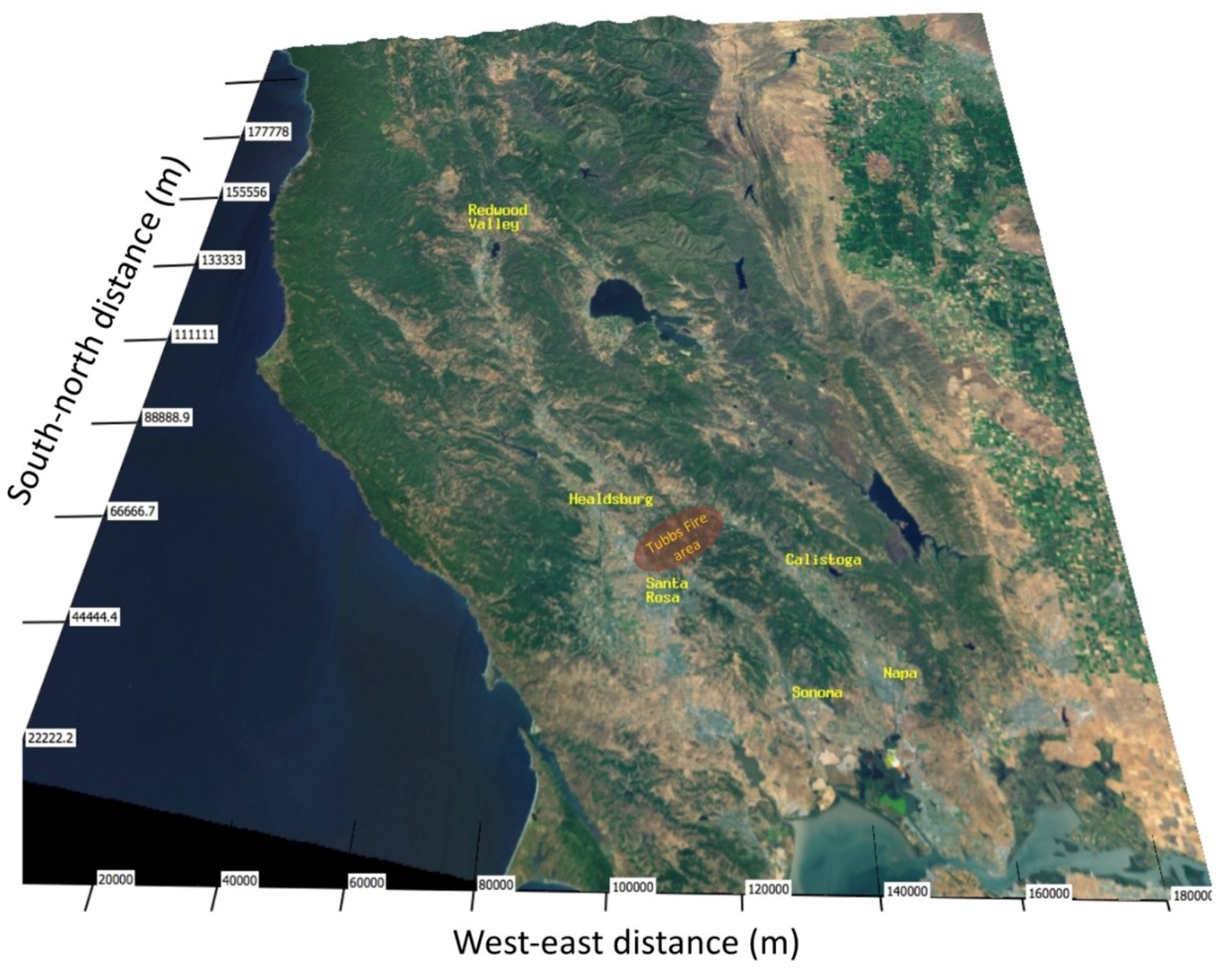
Three CAWFE configurations were employed in this work. First, in a weather-only simulation, three nested domains refined regional simulations from 10 km horizontal grid spacing to 3.3 km to 1.1 km over a 180 km × 200 km area covering the North Bay area, Sacramento Valley, and the mountains to its east (Figure 7), with vertical grid spacings of 43 m, 80 m, and 116 m, stretching to 322 m spacing at higher altitudes. The first half-grid level, where horizontal velocities are located according to the Arakawa C-grid staggering of variables, was at 21.6 m. This configuration was used to perform a weather-only simulation, initialized with the NAM forecast valid at 0600 UTC, 8 October (11 a.m., 8 October), that was used to explore the wind event leading to and occurring during the fire outbreak through 5 a.m., 9 October.
A second retrospective weather + fire research configuration further refined to the fourth and fifth domains, with horizontal grid spacings of 370 m and 185 m, respectively. The fifth domain was also vertically refined with near-surface vertical grid spacings of 17 m, 26 m, and 35 m, stretching to 161 m. This simulation, initialized with the NAM forecast valid at 9 October, 0000 UTC (5 p.m., 8 October), began at 7 p.m., ignited a fire at the reported time and location of the Tubbs Fire origin, and modeled the subsequent interactive weather and fire behavior for 30 h. The first half-grid level was at 8.5 m.
A final forecast weather plus fire configuration employed four nested domains, refining from 10 km to 370 m horizontal grid spacing using a 3:1 horizontal grid refinement and a 2:1 vertical grid refinement in domain 3 and again in domain 4. The finest domain used 72 × 72 grid points, with 44 vertical grid levels. The first half grid level was at 7.3 m. Vertical grid lengths stretched from 15 m to 125 m near the open top (3.3 km) of the innermost domain. The computational domains were centered on the Tubbs Fire ignition, i.e., they were not optimized using post-fire knowledge. This forecast began at 7 p.m. on 8 October using the 0000 UTC 9 October forecast, the most recent NAM forecast available when fires were detected, and extended for 34 h.
The spatial fuel variability for all simulations was specified with 2014 LANDFIRE (www.landfire.gov) data [37] using 13 fire behavior fuel models, based on the Albini [38] classification system as restated by Anderson [33]. The extent included urban zones, which (although considered unable to carry wildland fire, does so through landscape plants and materials and spotting), we have arbitrarily treated as grassy fuels. Lower elevation fuels were composed of short herbaceous types, herbaceous plants interspersed with shrubs, and short shrubs. The base of the slopes included shrubs with hardwoods, such as live oaks, particularly in drainages, while higher elevations are forested. The surface dead fuel moisture content, drawn from area Remote Automated Weather Station (RAWS) measurements, was specified as 4%, with a daily amplitude of 0.3%, and the live canopy fuel moisture content set at 57%, again based on local sources. Wind speeds at the height of the two lowest horizontal velocity components were extrapolated to fuel height. The arbitrary rate of spread cap originally assigned to rate of spread models as 5 m/s was raised to 20 m/s.
4. Results
4.1. Regional Winds
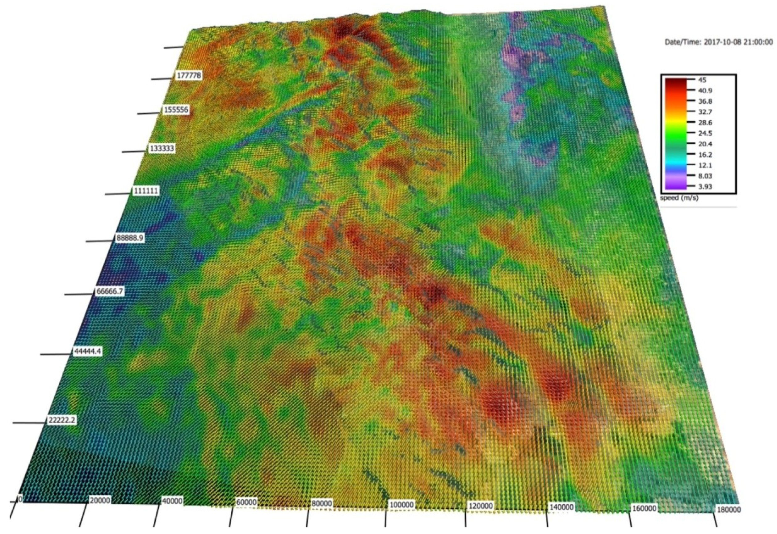
During 8 October into the early hours of 9 October, the regional weather simulation produced southwesterly Diablo winds in the northern coastal ranges, winds that travelled southwesterly down the slopes of the mountains on the east side of the Sacramento Valley, and winds that travelled south down the Sacramento Valley that then fanned out to the southwest over Wine Country. The strength of the winds waxed and waned and the direction wavered, creating broad areas (on the order of 10 km wide along a ridge) where wind overrunning topography reached 30–40 m/s, steady streaks or transient eddies of high speed air formed in the lee of some topographic features, and terrain created sheltered, low-speed areas downstream of others (Figure 8 and Video S1). Several of these high wind speed peaks were located near the upwind edge of wildfires. The simulated wind event subsided in some areas at midnight. In other areas such as the Tubbs Fire area, strong winds were simulated to have lasted until between 3 a.m. and 4 a.m. on 9 October, when they subsided in agreement with Santa Rosa-area surface weather stations.
4.2. Simulations of Microscale Wind Variability in Time and Space and Resulting Fire Behavior
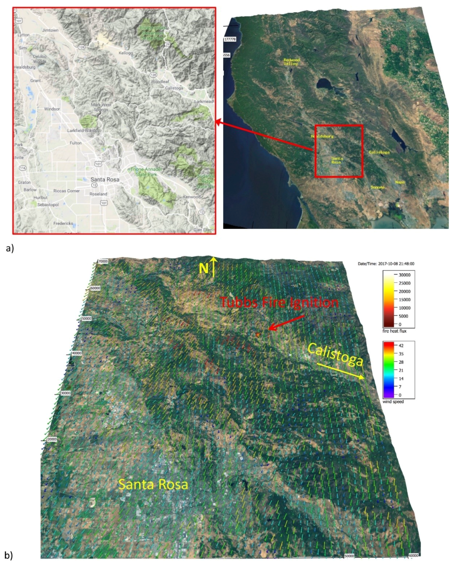
The second simulation refined the weather simulation to a fifth nested domain with 185 m horizontal grid spacing for the area shown in Figure 9a. The northwest two thirds of this domain spanned a river of disturbed air flowing off the ridge north and west of Calistoga, CA. Near-surface (8.5 m above ground level) modeled winds near the reported ignition time are shown in Figure 9b. Moderate winds entering the domain from the northeast accelerated over broad, taller ridges (≈500 m above surrounding elevations), yet the strongest accelerations were located at secondary, shorter topographic features (≈100–200 m above surrounding elevations) downstream. At 9:48 p.m., locations of near-surface winds reaching 35–42 m/s coincided with the area of the Tubbs fire ignition and hills downstream (Figure 9b). An animated sequence of near-surface winds (Video S2) shows these small (1.1–1.7 km diameter) patches of extreme winds formed over the top of secondary topographic features and broke off, flowing downstream. As the strength of incoming winds surged and subsided with a period of 5–7 min, the direction varied slightly, amidst a general shift of incoming winds from 28° to 41° from north, reflecting the changing pressure environment shown in Figure 2.
Evaluating the realism of the flow regime produced by microscale simulations is challenging, as the spatial variability of flow features was an order of magnitude finer than the distance between surface stations. The reporting of several-minute mean wind speeds (depending on the station and reporting) and gusts (the peak wind measured within a time period) can be difficult to interpret when the flow is characterized by coherent bursts on the order of a few minutes apart. In addition, the instantaneous vertical profile in wind speed may not be well represented by standard approximations such as the logarithmic profile, several of the assumptions behind which are not met in these conditions.
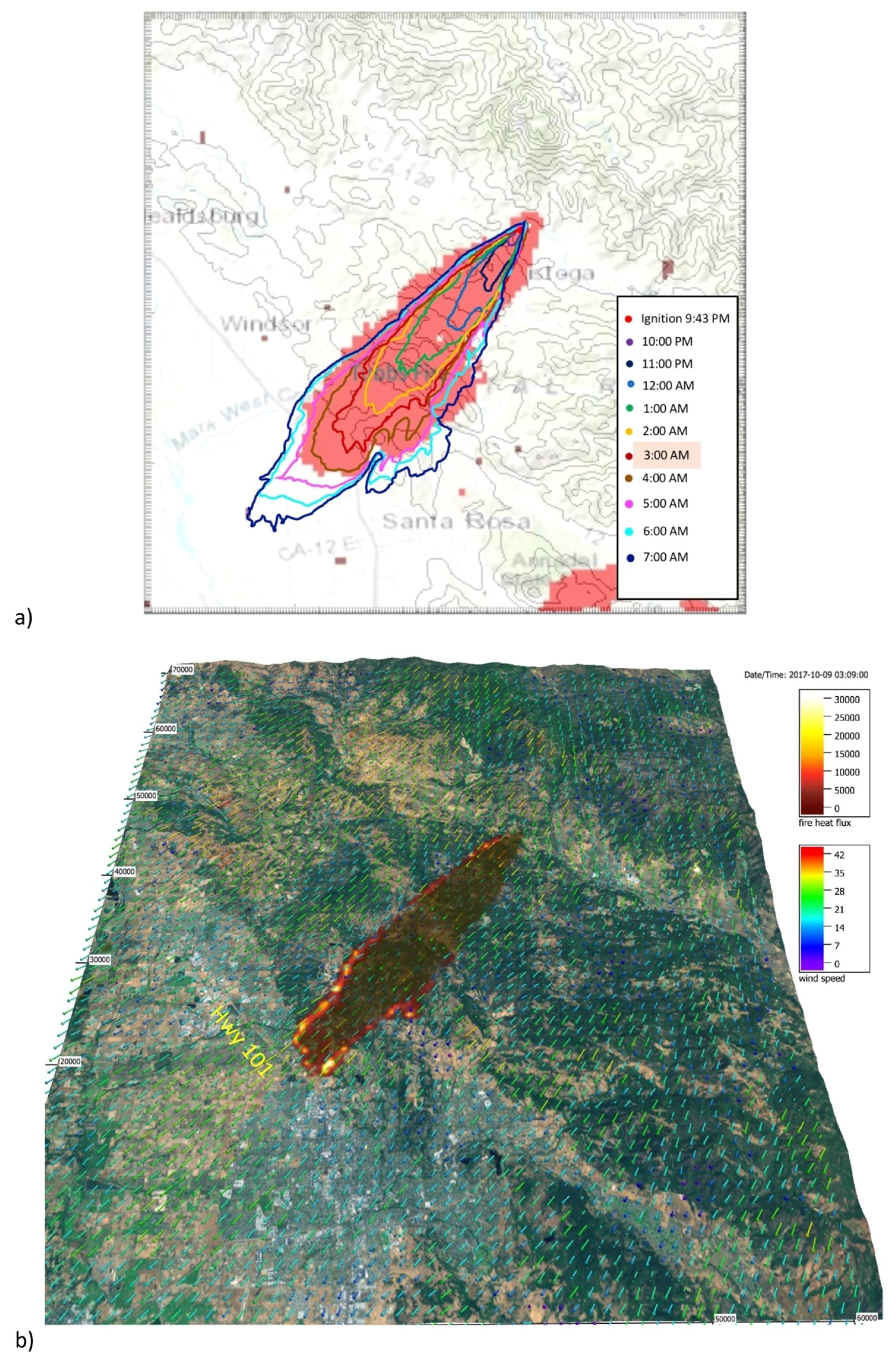
The simulated fire line progression, included in Video S2 and plotted versus the active fire area detected by VIIRS at 3:09 a.m. in Figure 10a, reproduced the observed direction of the fire and an extremely rapid spread. However, the simulation produced an average spread rate of 0.86 m/s by reaching Highway 101, 17 km away, in 5.5 h versus the 4.5 h time at which heat signatures detected by VIIRS were reported. If the detected heat signatures represent the extent reached by the flaming front (which is uncertain, as extensive spotting was reported), the simulation underestimated the actual average rate of spread of 1.05 m/s reported over this period. Late in the simulated period, the southern flank was drawn perpendicular to the airflow over topography to the southeast, expanding the fire width by 2 km; the simulation reproduced this type of growth when it reached the topographic feature, though this was correspondingly later than observed. This outward bowing of the fire line spreads upwind up the fire line throughout the simulated period.
4.3. Vertical Structure of Wind Speed
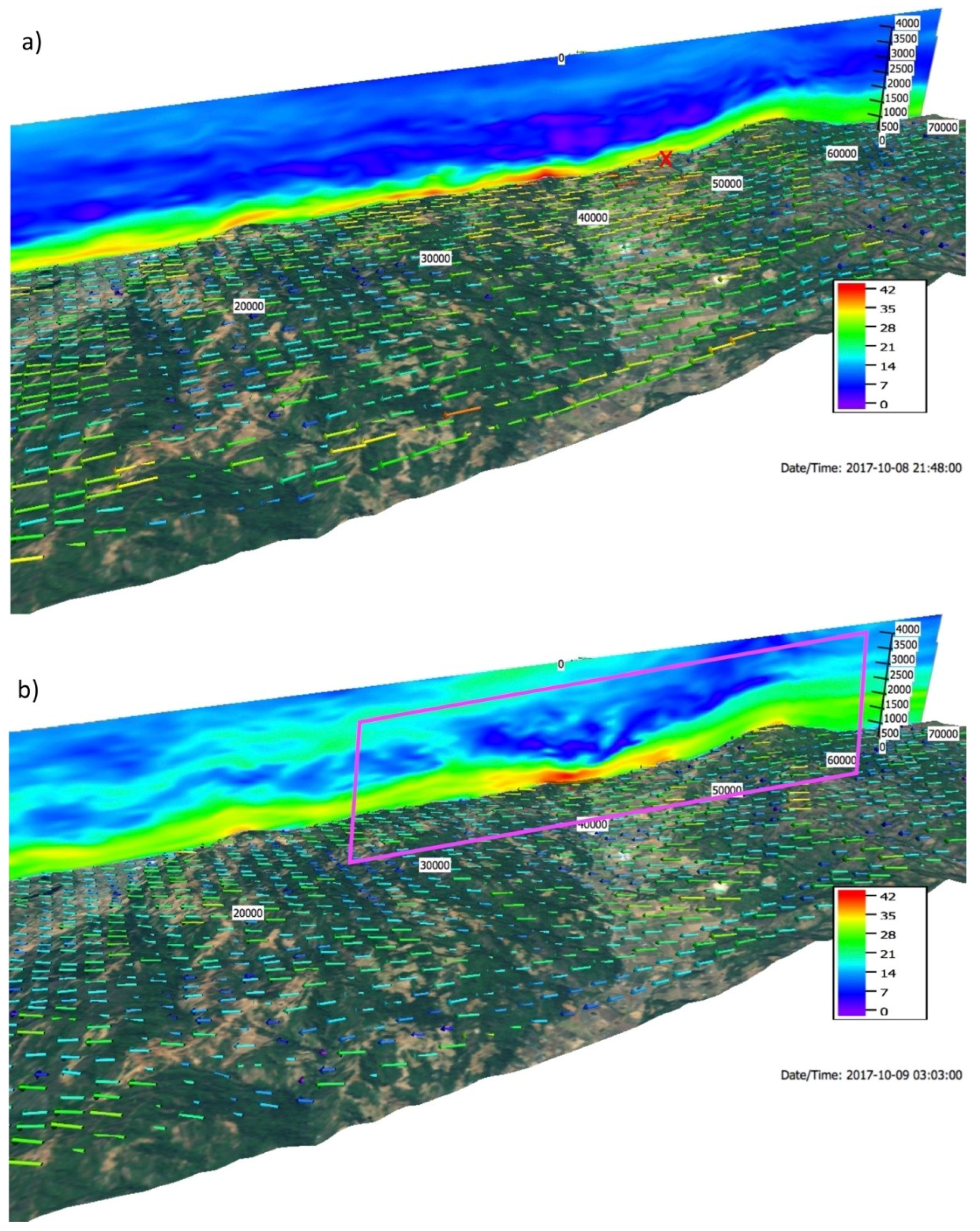
Near the estimated ignition time, a vertical cross-section of wind speed in the plane oriented along the flow through the reported ignition point showed a shallow 1.25–1.4 km deep layer of high speed (greater than 20 m/s) air, punctuated by higher simulated wind speeds over the crest of hills (Figure 11). Those wind speeds reached 32 m/s over the taller upstream hill upwind of the ignition point, but were greater, reaching 35–42 m/s over the subsequent lesser hills, including near the ignition (indicated on Figure 11a). An animation (Video S3) shows that these high wind speed peaks over crests of lower hills created streaks or bursts of high speed air breaking off and traveling downstream at approximately 5–7-min intervals, a similar feature and frequency to pulses produced in the near-surface stable layer that occurred in simulations of the Santa Ana-driven Esperanza wildfire [11] and Front Range windstorms [17]. At times, the flow in this case resembled a hydraulic jump (Figure 11b), a location where the peak wind increased and the depth of the high-speed zone decreased, creating a transition between smoother upstream air and turbulent motions downwind. The turbulent motions lay at the horizontal interface between the high-speed surface zone and less stable, slower moving layer above. Viewed in motion (Video S3), the depression of the jump varied in time. Despite the strongly stable layer in the lowest 1.5 km and stable stratification throughout the lower atmosphere, the simulations did not present evidence of propagating waves, instead, the peaks at the crest of small knolls resembled neutrally stratified flow over small hills but produced pulses of high speed air breaking off and traveling downwind. The flow direction changed over this period, thus, by the end of the sequence, the flow had rotated approximately 12° into the plane. The flow began to weaken by 4 a.m.
The Froude number (Equation (1)) is an imperfect indicator in a continuously stratified fluid (i.e., a fluid with multiple layers of stratification) and complex environment. The above environmental parameters for N and θ, large (500 m) and small (100 m) hills in 30 m/s flow yielded approximate Fr of 4 and 20, respectively. While both exceed 1 and thus lay in the supercritical flow regime, the particularly high value for small hills indicated that horizontal momentum effects greatly exceeded buoyancy effects. This analysis supports the result that for very high-speed flow across small hills, the flow might be expected to behave as if it were neutrally stratified, producing a minimum in the induced surface pressure accompanied by a maximum in the near-surface wind speed across the hilltop, but that simple analysis does not predict the result that pulses of wind that break off and travel downwind in the lee.
4.4. Forecast Configuration
In configuring a forecast (versus a retrospective research simulation), additional constraints are that (1) the simulation must balance fidelity with time constraints that may not allow optimal configuration (e.g., limits on resolution or size of the domain); (2) rely only on data available at the time the simulation uses it; and (3) balance complexity (e.g., having many steps in the process, the proximity to numerical stability limits, and degree of computational needs) with robustness. Our operational concept was that, given a time and location for an ignition, the most recent NAM forecast data that was available would initialize a CAWFE simulation relying on information known at the time. The CAWFE simulation was configured as a forecast with four nested domains sequentially telescoping to 370 m horizontal grid spacing, with the innermost domain spanning 26.7 × 26.7 (large enough to encompass nearly all wildland fires) × 3.3 km beginning with the NAM’s forecast for 7 p.m. on 8 October. The top of the innermost domain is an open boundary through which air motions may pass, so this is not a lid, but merely defines the top of the volume that may be further refined both horizontally and vertically. This simulation might be seen as the first of a sequence of simulations using the cycling forecast paradigm for fire modeling that was put forth in Reference [39]; however, in this case, the reported fire ignition was used as the initial location, rather than satellite active fire detection data. This was done because the first data was provided via VIIRS at 3:09 a.m., after the first growth surge.
Compared to previous configurations, the vertical grid length was stretched in the outer domains to reduce the number of grid points and make the configuration less likely to have numerical instabilities. Assuming no prior knowledge of the fire growth direction or speed, the domains were centered on the reported ignition point. In this configuration, when all four domains were activated, the calculations proceeded at four times faster than real time on a single computer processor (Intel®Xeon® CPU E5-2667 v4 @ 3.20 GHz) of a Linux x86_64 workstation. Previous work (e.g., Reference [40]) asserted that numerical weather prediction model-based fire behavior models are not suitable as forecasting tools because of the computational cost. Indeed, other coupled weather-fire models based upon the Weather Research and Forecasting model have reported a need for much greater computational resources. For example, Reference [41] used 120 processors to achieve 500 m grid spacing at speeds that broach faster than real time for a large fire, while Reference [42] report producing an 18-h forecast in about 4 h on 24 processors, apparently referring to a configuration that refined to a 110 m horizontal grid spacing over a 13 km × 13 km domain.
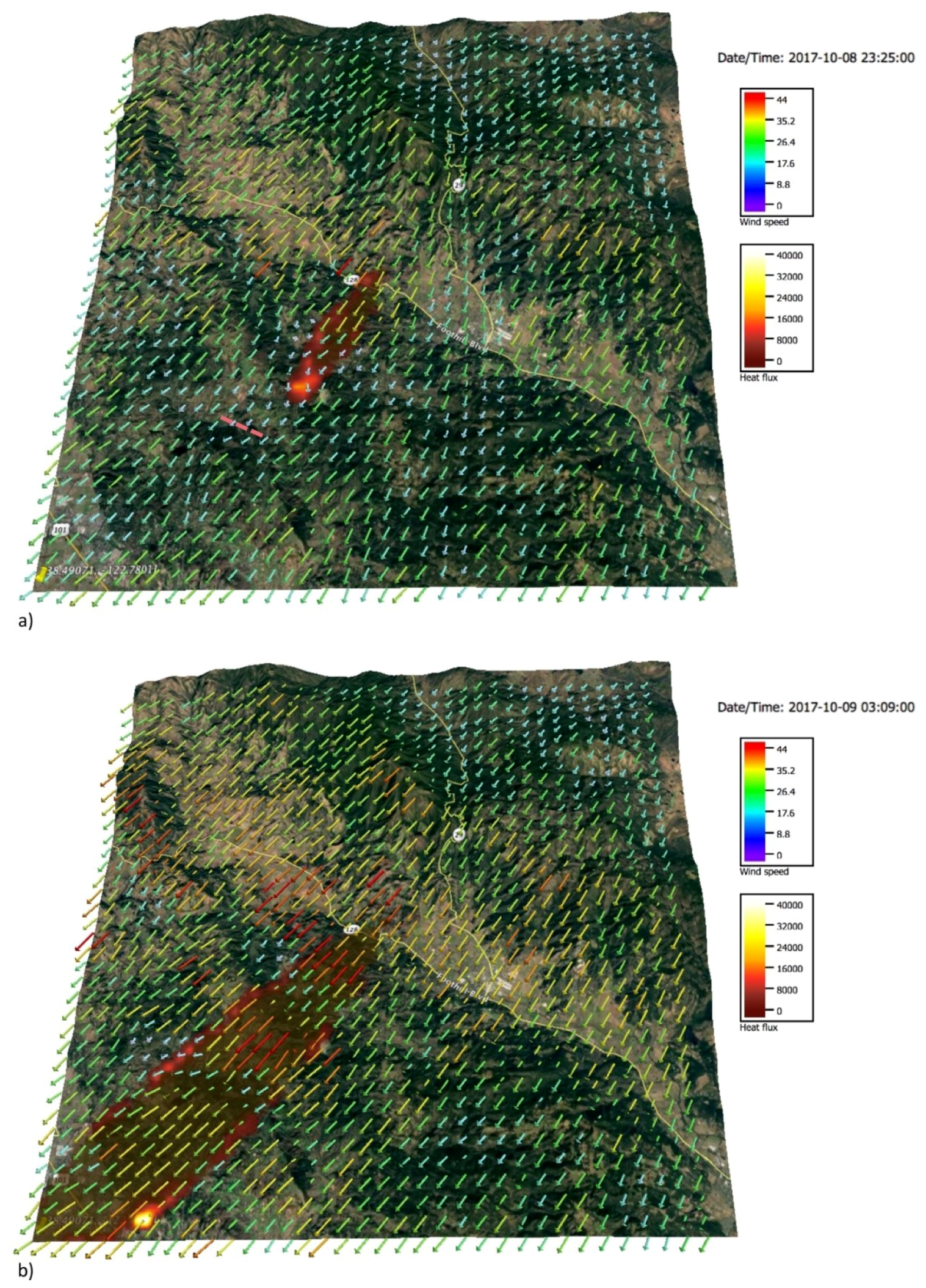
Simulations using this forecast configuration, shown in Figure 12, correctly captured an elliptically-shaped rapid fire progression to the southwest. In comparison with the earliest satellite active fire detections (Figure 6), the forecast configuration (Figure 12a) underestimated the fire’s growth from ignition to MODIS’ mapped fire extent at 11:25 p.m. (Figure 6). In addition, it predicted the fire extended beyond Highway 101 by 3:09 p.m. on 9 October (Figure 12b), in agreement with the VIIRS active fire detection data (Figure 6), although the simulated fire’s heading region had grown out of domain 4’s boundaries. An animation of near surface winds and fire progression for this simulation (Video S4) also showed high wind speed peaks over secondary ridges exceeding 35 m/s and in some areas, exceeding 40 m/s. The wind speed peaks exceeded the previous simulation by 3–5 m/s and broke away at a higher frequency, approximately every 4 min., compared to 5–7 min in the five-domain research configuration. The arrival time is more “on time” than the research simulation; however, this could be overpredicting the rate of spread of the flaming front as ember spotting was widely reported with this fire and could account for reports of fire arrival time and satellite-based active fire detection at the leading edges, rather than the progression of a flaming front.
5. Discussion
This work examines the structure of topographically-altered airflow within a case of Diablo winds associated with a widespread fire outbreak in the coastal and inland mountains north of San Francisco Bay in October 2017. Because surface weather station data was sparse and largely missed extreme winds that anecdotal reports suggest occurred, the large-scale synoptic environment was changing throughout the event, and the three-dimensional topography was too complex for analytical solutions, numerical simulations refining from mesoscale to microscale were used to examine the flow regime. When two-way coupled with a fire behavior module—a system validated on previous fires in diverse conditions—CAWFE simulations reproduced many aspects of the unfolding fire event. In showing that observed regional Diablo winds accelerated further over broad ridges in the North Bay, varying throughout the day in strength and direction and creating leeward streaks and pulses of higher wind speeds, the simulations provided a coherent framework for understanding the patterns and variability in the surface station data.
Previous work (e.g., Reference [8]) has described the regional environmental conditions that indicate and induce strong Diablo winds. Here, research simulations with refined resolution gave further insight into the locations and possible mechanisms for the generation of hypothesized extreme winds within these streaks and pulses—not, as might be anticipated, on the highest ridges, but on hills in the lee of the larger ridges, including near the Tubbs fire ignition site, and in bursts that periodically break off and travel downstream from these secondary hills. The airflow pattern showed aspects of previously studied regimes including transient resemblance to a hydraulic jump, but, as the dimensional analysis of flow parameters support, some of the most extreme winds occur over secondary hill crests. Previous conjectures that stable high-speed flow would behave as though it were neutrally-stratified flow over small hills, producing winds peaks at secondary hill crests despite a near-surface stable layer, were largely borne out but that analysis did not predict the production of the periodic wind bursts. A previous numerical modeling study of a Front Range downslope wind storm [17] produced similar behavior—bursts of high speed wind breaking off in the mountains’ lee—of similar periodicity, but the authors’ attribution of the phenomena to wave breaking does not apply here; a simpler explanation may underlie both.
As these simulations are performed at resolutions more than an order of magnitude finer than numerical weather prediction forecasts, it may be asked whether such features—well beneath what operational forecasts currently can resolve—can be anticipated with modern computational resources. Assertions have been widely made that coupled models cannot be used in a forecast sense because of the computational demands that would be required, while understanding within the meteorological community states that predictability decreases at finer scales as one approaches the boundary layer regime, where key features cannot be predicted deterministically at all [43]. We show, as a practical disproof, that the coupled system, configured as a generally applicable forecast rather than optimized for this case, can be run four times faster than real time for a large fire at high resolution on a single processor of a workstation, reproducing the important aspects of the flow regime and providing a good reproduction of the accompanying fire growth. Previous work [44] showed that, provided that the simulation can reproduce winds at hundreds of meters and include feedbacks from the fire on the local winds (a lesser factor in wind-driven fires [11]), many aspects of fire behavior are understandable and predictable. Here, we additionally show a practical implication: at least using this model, such computations are fast enough even without multiprocessor supercomputers to be used with sufficient resolution and have good skill as a forecast for large wildfires.
Some points remain unsettled in the reproduction or prediction of winds. The features modeled occurred at scales that may lie between or slightly miss observations, preventing direct verification of extreme small-scale motions or winds at secondary peaks. In addition, their size is beneath the scales that operational forecast models can resolve, limiting the ability to reproduce the extreme winds with current operational models and configurations. The temporal frequency (4–7 min) of bursts in the lee of topographic features are difficult to reconcile with reported winds, which are reported (depending on the equipment, network, and sampling frequency) as several minute averages and gusts. In addition, widely used methods, such as the logarithmic wind profile for vertically adjusting results to measurement heights or other heights of interest, rely on assumptions (e.g., that the stratification is neutral and the flow is stationary) that are not strictly met and may not accurately represent the vertical structure of wind speeds in downslope wind conditions.
Additional issues remain in the prediction of fire growth. Some or all of these could account for the differences between modeled and observed spread rates. First, the use of a flaming front to represent fire spread does not include the role of long distance ember spotting. Fire brands can play many roles in wildland fires, from short-distance spotting ahead of the line where they may be overrun by the flaming front before they can develop their own circulations, or the rarer long-distance spotting kilometers ahead of the line, where they might ignite another fire, or as has been described in recent windstorm-driven fires, the fire itself may be described as traveling as a storm of embers. The treatment of spotting in coupled model simulations of landscape-scale events has been a broad-brush attempt to claim the more rapid rates of spread this provides while overlooking the details and distinctions between these roles. For example, short-distance spotting is assumed to be part of the processes moving the flaming front ahead, processes that are parameterized with relationships like Reference [29]. Long-distance spotting has been treated as resulting from the resolved-scale winds, perhaps with stochastic components to achieve the apparent randomness, though deterministic prediction of the specific location and timing of the occasional ember is not realistic. Observations have not determined critical aspects of ember storms, which present an intermediate case and it is uncertain if they draw air currents that may impact the upcoming fire line or get overrun, having no impact of subsequent fire spread. Fire growth due spotting depends on the ember density, how favorable conditions are for ignition where they land, and the heat flux they produce. Because VIIRS could detect these fires as soon as they reach one to a few meters in size, or even a storm of a sufficient number of embers whether or not they have ignited other materials, spotting complicates the interpretation of the fire extent from active fire detection data, in addition to muddying the interpretation of anecdotal reports on where the fire is. Therefore, in these conditions, it is not clear if variance in simulated fire extent, which means the extent of the flaming front, from the observed fire extent is an error from the location of the actual flaming front, or if detections indicated the extent of embers, which may or may not have been participating in propagation of the fire. Thus, the lag in modeled fire spread in Figure 10 with respect to reports or detections may correctly represent a difference in extent of the flaming front and embers further ahead.
Second, the empirical rate of spread relationships such as that of Reference [29] have not been validated at extreme wind speeds. Third, initiation of fire growth forecasts can begin when a fire is detected or reported. In this case, which reported ignition occurred near 9:45 p.m., the first detection by the VIIRS data was produced 5 h later at 3:09 a.m., as the first rapid growth period was ending. Fourth, weather models must also make assumptions about the vertical profile of wind in the atmospheric surface layer; though widely used anyway, the assumptions under which these profiles were developed are not supported in stable, topographically-varying, temporally changing conditions. Finally, the leading edge of the simulated fire traveled fast enough to exit the CAWFE domain showing limits in this approach as currently applied for the detection and forecast of very fast-moving fires.
6. Conclusions
We found that as high speed regional flow of the type called Diablo winds varied in strength and direction, it created flow patterns that resembled previously studied regimes. However, because of the complex multi-scale topography and evolving synoptic situation, that flow contained some surprising aspects such as streaks and bursts in the lee of some topographic features and stagnation downstream of others. Diablo winds alone were not sufficient to explain extreme winds, nor was their general acceleration over broad hills; instead, the regional pattern and mesoscale (2–20 km) acceleration amplified at small hills, under 2 km wide with heights of a few hundred meters over surrounding terrain, creating exceptional peaks of 30–40 m/s over these secondary, lower hill crests; under a transient feature sometimes resembling a hydraulic jump; and in bursts breaking off and traveling downstream at approximately 5–7-min intervals. The acceleration over secondary hill peaks occurred because in very high Froude number flow, stability effects are diminished and the flow behaves much like neutrally stratified flow over a small hill, though the shedding of bursts of high speed air is not anticipated by that simple analysis. The transience in those peaks and the bursts traveling downstream could be consistent with the variability in data in (Figure 3, Figure 4 and Figure 5) from local weather stations in the APRSWNET/CWOP network, for which data is available at higher frequency. The cumulative effect of the complex multi-scale airflow was to reproduce fire arrival times, direction, and shape including growth perpendicular to a flank when the fire reaches a topographic feature and draws itself up.
CAWFE coupled weather and fire growth simulations reproduced the fire shape and rapid growth. A detailed retrospective research simulation lagged observed fire line progression, predicting arrival at Santa Rosa 1 h after satellite active fire detections recorded ignitions there. Another CAWFE simulation configured as a forecast at 370 m horizontal grid spacing produced slightly faster arrival in line with observations, with calculations proceeding at 4 times faster than real time on a single computer processor. The significance is that CAWFE forecasts much finer than operational weather forecasts can anticipate extreme winds as well as fire growth. As the magnitude of extreme winds are often a critical predictive metric, this model may have application to understanding and anticipating high-impact fine-scale wind extrema in applications such as anticipating impacts on utility infrastructure and other phenomena, such as Front Range windstorms and landfalling hurricanes.
Supplementary Materials
The following are available online at https://www.mdpi.com/2073-4433/9/12/462/s1, Video S1: S1.mp4, Video S2: S2.mp4, Video S3: S3.mp4, Video S4: S4.mp4.
Author Contributions
Conceptualization, J.C. and W.S.; Data curation, B.Q.; Funding acquisition, J.C. and W.S.; Investigation, J.C. and W.S.; Methodology, J.C. and W.S.; Project administration, W.S.; Software, J.C.; Validation, J.C., W.S., and B.Q.; Visualization, J.C.; Writing—original draft, J.C. and W.S.; Writing—review and editing, J.C., W.S., and B.Q.
Funding
This material is based upon work supported by NASA under Award NNX12AQ87G and FEMA under Award EMW-2015-FP-00888.
Acknowledgments
NCAR is sponsored by the National Science Foundation. We thank Peter Sullivan for helpful conversations regarding the simulation of atmospheric flow regimes.
Conflicts of Interest
The authors declare no conflict of interest. The funders had no role in the design of the study; in the collection, analyses, or interpretation of data; in the writing of the manuscript, or in the decision to publish the results.
References
- CAL FIRE Investigation Report, Case Number 17 CALNU 010049, Case Name Nuns; California Department of Forestry and Fire Protection: Sacramento, CA, USA, 8 October 2017. Available online: http://calfire.ca.gov/fire_protection/downloads/FireReports/Nuns%20LE%2080_Redacted.pdf (accessed on 30 June 2018).
- CAL FIRE Investigation Report, Case Number 17CAMEU012169, Case Name Redwood Incident; California Department of Forestry and Fire Protection: Sacramento, CA, USA, 8 October 2017. Available online: http://calfire.ca.gov/fire_protection/downloads/FireReports/LE-80%20Redwood%20Incident%20Report_Redacted.pdf (accessed on 30 June 2018).
- Monteverdi, J. The Santa Ana weather type and extreme fire hazard in the Oakland-Berkeley Hills. Weatherwise 1973, 26, 118–121. [Google Scholar] [CrossRef]
- Null, J. Weather Corner. San Jose Mercury News, 26 October 1999. [Google Scholar]
- Pagni, P.J. Causes of the 20 October 1991 Oakland Hills conflagration. Fire Saf. J. 1993, 21, 331–339. [Google Scholar] [CrossRef]
- Van Niekerken, B. Wine Country Fire of 1964: Eerie Similarities to this Week’s Tragedy. San Francisco Chronicle. 10 October 2017. Available online: https://www.sfchronicle.com/thetake/article/Wine-Country-fire-of-1964-Eerie-similarities-to-12267643.php (accessed on 31 October 2017).
- Smith, C.; Hatchett, B.; Kaplan, M. Characteristics of Diablo-like Wind conditions in Northern California Based on a Climatology from Surface Observations. Preprints 2018, 1, 25. [Google Scholar] [CrossRef]
- Bowers, C.L.; Clements, C.B. The Diablo Winds of Northern California: Climatology, Severity, and Spatial Characteristics. J. Geophys. Res. Atmos. 2018. submitted. [Google Scholar]
- Nausler, N.J.; Abatzoglou, J.T.; Marsh, P.T. The 2017 North Bay and Southern California Fires: A Case Study. Fire 2018, 1, 18. [Google Scholar] [CrossRef]
- California Public Utilities Commission. PG&E Fire Incident Reports. Available online: http:// http://cpuc.ca.gov/general.aspx?id=6442455196 (accessed on 30 June 2018).
- Coen, J.L.; Riggan, P.J. Simulation and thermal imaging of the 2006 Esperanza wildfire in southern California: Application of a coupled weather-wildland fire model. Int. J. Wildland Fire 2014, 23, 755–770. [Google Scholar] [CrossRef]
- Gohm, A.; Zängl, G.; Mayr, G.J. South Foehn in the Wipp Valley on 24 October 1999 (MAP IOP 10): Verification of high-resolution numerical simulations with observations. Mon. Weather Rev. 2004, 132, 78–102. [Google Scholar] [CrossRef]
- Cao, Y.; Fovell, R.G. Downslope windstorms of San Diego County. Part I: A case study. Mon. Weather Rev. 2016, 144, 529–552. [Google Scholar] [CrossRef]
- Colle, B.A.; Mass, C.A. Windstorms along the Western Side of the Washington Cascade Mountains. Part I: A High-Resolution Observational and Modeling Study of the 12 February 1995 Event. Mon. Weather Rev. 1998, 126, 28–52. [Google Scholar] [CrossRef]
- Colle, B.A.; Mass, C.A. Windstorms along the Western Side of the Washington Cascade Mountains. Part II: Characteristics of Past Events and Three-dimensional Idealized Simulations. Mon. Wea. Rev. 1998, 26, 52–71. [Google Scholar] [CrossRef]
- Clark, T.L.; Peltier, W.R. On the evolution and stability of finite-amplitude mountain waves. J. Atmos. Sci. 1977, 34, 1715–1730. [Google Scholar] [CrossRef]
- Scinocca, J.F.; Peltier, W.R. Pulsating downslope windstorms. Pulsating downslope windstorms. J. Atmos. Sci. 1989, 46, 2885–2914. [Google Scholar] [CrossRef]
- Wilson, J.D. Measured and modelled wind variation over irregularly undulating terrain. Agric. For. Meteorol. 2018, 249, 187–197. [Google Scholar] [CrossRef]
- Hunt, J.C.R.; Richards, K.J. Stratified Airflow over One or Two Hills. In Boundary Layer Structure; Kaplan, H., Dinar, N., Eds.; Springer: Dordrecht, The Netherlands, 1984; ISBN 978-94-009-6516-4. [Google Scholar]
- Finnigan, J.J. Air Flow Over Complex Terrain. In Flow and Transport in the Natural Environment: Advances and Applications; Steffen, W.L., Denmead, O.T., Eds.; Springer: Berlin/Heidelberg, Germany, 1988; ISBN 978-3-642-73847-0. [Google Scholar]
- Miller, C.; Gibbons, M.; Beatty, K.; Boissonnade, A. Topographic speed-up effects and observed roof damage on Bermuda following Hurricane Fabian (2003). Mon. Weather Rev. 2013, 28, 159–174. [Google Scholar] [CrossRef]
- Fernando, H.J.S.; Pardyjak, E.R.; Di Sabatino, S.; Chow, F.K. The MATERHORN: Unraveling the intricacies of mountain weather. Bull. Am. Meteorol. Soc. 2015, 96, 1945–1967. [Google Scholar] [CrossRef]
- Brighton, P.W.M. Strongly stratified flow past three-dimensional obstacles. Quart. J. R. Meteorol. Soc. 1978, 104, 289–307. [Google Scholar] [CrossRef]
- Clark, T.L.; Keller, T.; Coen, J.; Neilley, P.; Hsu, H.; Hall, W.D. Terrain-induced Turbulence over Lantau Island: 7 June 1994 Tropical Storm Russ Case Study. J. Atmos. Sci. 1997, 54, 1795–1814. [Google Scholar] [CrossRef]
- Clark, T.L.; Hall, W.D.; Coen, J.L. Source Code Documentation for the Clark-Hall Cloud- Scale Model Code Version G3CH01; NCAR Technical Note NCAR/TN-426+STR; NCAR: Boulder, CO, USA, 1996. [Google Scholar]
- Coen, J. L. Some requirements for simulating wildland fire behavior using insight from coupled weather-wildland fire models. Fire 2018, 1, 6. [Google Scholar] [CrossRef]
- Coen, J.L. Simulation of the Big Elk Fire using coupled atmosphere—Fire modeling. Int. J. Wildland Fire 2005, 14, 49–59. [Google Scholar] [CrossRef]
- Coen, J.L. Modeling Wildland Fires: A Description of the Coupled Atmosphere-Wildland Fire Environment Model (CAWFE); NCAR Technical Note NCAR/TN-500+STR; NCAR: Boulder, CO, USA, 2013. [Google Scholar]
- Rothermel, R.C. A Mathematical Model for Predicting Fire Spread in Wildland Fuels; Research Paper INT-115; USDA Forest Service, Intermountain Forest and Range Experiment Station: Ogden, UT, USA, 1972.
- Van Wagner, C.E. Conditions for the start and spread of crown fire. Can. J. For. Res. 1977, 7, 23–34. [Google Scholar] [CrossRef]
- Rothermel, R.C. Predicting Behavior and Size of Crown Fires in the Northern Rocky Mountains; Research Paper INT-438; USDA Forest Service: Ogden, UT, USA, 1991.
- Koo, E.; Linn, R.R.; Pagni, P.; Edminster, C. Modeling firebrand transport in wildfires using HIGRAD/FIRETEC. Int. J. Wildland Fire 2012, 21, 396–417. [Google Scholar] [CrossRef]
- Anderson, H.E. Aids to Determining Fuel Models for Estimating Fire Behavior; USDA Forest Service, Intermountain Forest and Range Experiment Station, General Technical Report INT-122; USDA: Ogden, UT, USA, 1982.
- Scott, J.H.; Burgan, R.E. Standard Fire Behavior Fuel Models: A Comprehensive Set for Use with Rothermel’s Surface Fire Spread Model; USDA For. Serv. Gen. Tech. Rep. RMRS-GTR-153; USDA: Ogden, UT, USA, 2005.
- Ottmar, R.D.; Sandberg, D.V.; Riccardi, C.L.; Prichard, S.J. An overview of the Fuel Characteristic Classification System—Quantifying, classifying, and creating fuelbeds for resource planning. Can. J. For. Res. 2007, 37, 2383–2393. [Google Scholar] [CrossRef]
- Coen, J.L.; Stavros, E.N.; Fites-Kaufman, J.-A. Deconstructing the King megafire. Ecol. Appl. 2018. [Google Scholar] [CrossRef] [PubMed]
- LANDFIRE. Existing Vegetation Type Layer, LANDFIRE 1.1.0, U.S. Department of the Interior, Geological Survey. 2008. Available online: http://landfire.cr.usgs.gov/viewer/ (accessed on 28 October 2010).
- Albini, F.A. Estimating Wildfire Behavior and Effects; USDA Forest Service Intermountain Forest and Range Experiment Station, General Technical Report INT-30; USDA: Ogden, UT, USA, 1976.
- Coen, J.L.; Schroeder, W. Use of spatially refined remote sensing fire detection data to initialize and evaluate coupled weather-wildfire growth model simulations. Geophys. Res. Lett. 2013, 40, 5536–5541. [Google Scholar] [CrossRef]
- Forthofer, J.M.; Butler, B.W.; Wagenbrenner, N.S. A comparison of three approaches for simulating fine-scale surface winds in support of wildland fire management. Part I. Model formulation and comparison against measurements. Int. J. Wildland Fire 2014, 23, 969–981. [Google Scholar] [CrossRef]
- Kochanski, A.K.; Jenkins, M.A.; Mandel, J.; Beezley, J.D.; Krueger, S.K. Real time simulation of 2007 Santa Ana fires. For. Ecol. Manag. 2013, 294, 136–149. [Google Scholar] [CrossRef]
- Kosovic, B.; Mahoney, W.P.; Brown, B.G.; Cowie, J.R.; Anderson, A.; Boehnert, J.; Bresch, J.; Jimenez, P.A.; Munoz-Esparza, D.; Petzke, W.; et al. Advancements in Operational Wildland Fire Prediction; NCAR Day of Networking and Discovery 2017; National Center for Atmospheric Research (NCAR): Boulder, CO, USA, 2017. [Google Scholar]
- Mukherjee, S.; Schalkwijk, J.; Jonker, H.J.J. Predictability of dry convective boundary layers: An LES study. J. Atmos. Sci. 2016, 73, 2715–2727. [Google Scholar] [CrossRef]
- Coen, J.L.; Schroeder, W. The High Park Fire: Coupled weather-wildland fire model simulation of a windstorm-driven wildfire in Colorado’s Front Range. J. Geophys. Res. Atmos. 2015, 120, 131–146. [Google Scholar] [CrossRef]
Figure 1.
8–9 October 2017 wildfires. Satellite active fire detections revealed by the Suomi National Polar-orbiting Partnership Visible Infrared Imaging Radiometer Suite (S-NPP/VIIRS) at 3:09 A.M. Fire names are shown in purple italics.
Figure 1.
8–9 October 2017 wildfires. Satellite active fire detections revealed by the Suomi National Polar-orbiting Partnership Visible Infrared Imaging Radiometer Suite (S-NPP/VIIRS) at 3:09 A.M. Fire names are shown in purple italics.

Figure 2.
Hourly mean for the National Centers for Environmental Prediction (NCEP) North American Regional Reanalysis composites interpolated to 0.3 × 0.3 degrees for (a) surface pressure at 8 October, 12 UTC; (b) surface pressure at 9 October, 9 UTC; (c) 1000 mb vector wind at 9 October, 12 UTC; and (d) 1000 mb vector wind at 9 October, 9 UTC. Image provided by the National Oceanic and Atmospheric Administration (NOAA) Earth System Research Laboratory, Physical Science Division from their website at http://www.esrl.noaa.gov/psd/.

Figure 3.
Surface station map where station wind barbs show most recent wind observation within 1 h ending at 8 a.m. UTC 10/9/17. Selected stations, ordered by decreasing peak wind gusts (stations with higher peak gusts marked with squares and lower peak gusts marked with triangles), are located with colored polygons (according to table). Wind speed (blue) and wind gust (orange) data (in m/s) from HWCK1, which recorded the highest wind speeds. Wind station data is available at http://mesowest.utah.edu. Tubbs Fire extent at 3:09 a.m. on 9 October from VIIRS is shown in brown.

Figure 4.
Wind speed (blue) and wind gust (orange) data (in m/s) from surface stations located in Figure 3 that recorded moderate to high wind speeds.
Figure 4.
Wind speed (blue) and wind gust (orange) data (in m/s) from surface stations located in Figure 3 that recorded moderate to high wind speeds.
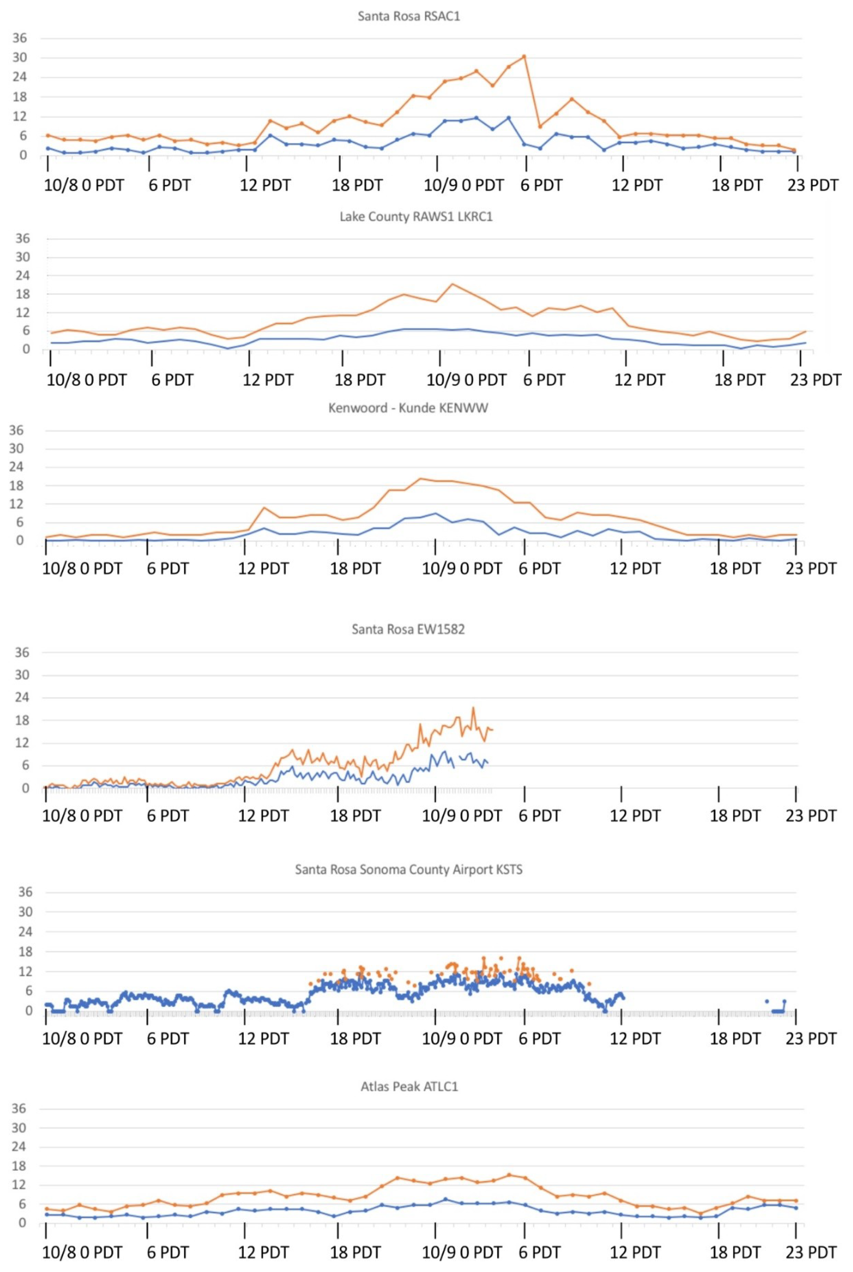
Figure 5.
Wind speed (blue) and wind gust (orange) data (in m/s) from surface stations located in Figure 3 that recorded weaker wind speeds.
Figure 5.
Wind speed (blue) and wind gust (orange) data (in m/s) from surface stations located in Figure 3 that recorded weaker wind speeds.
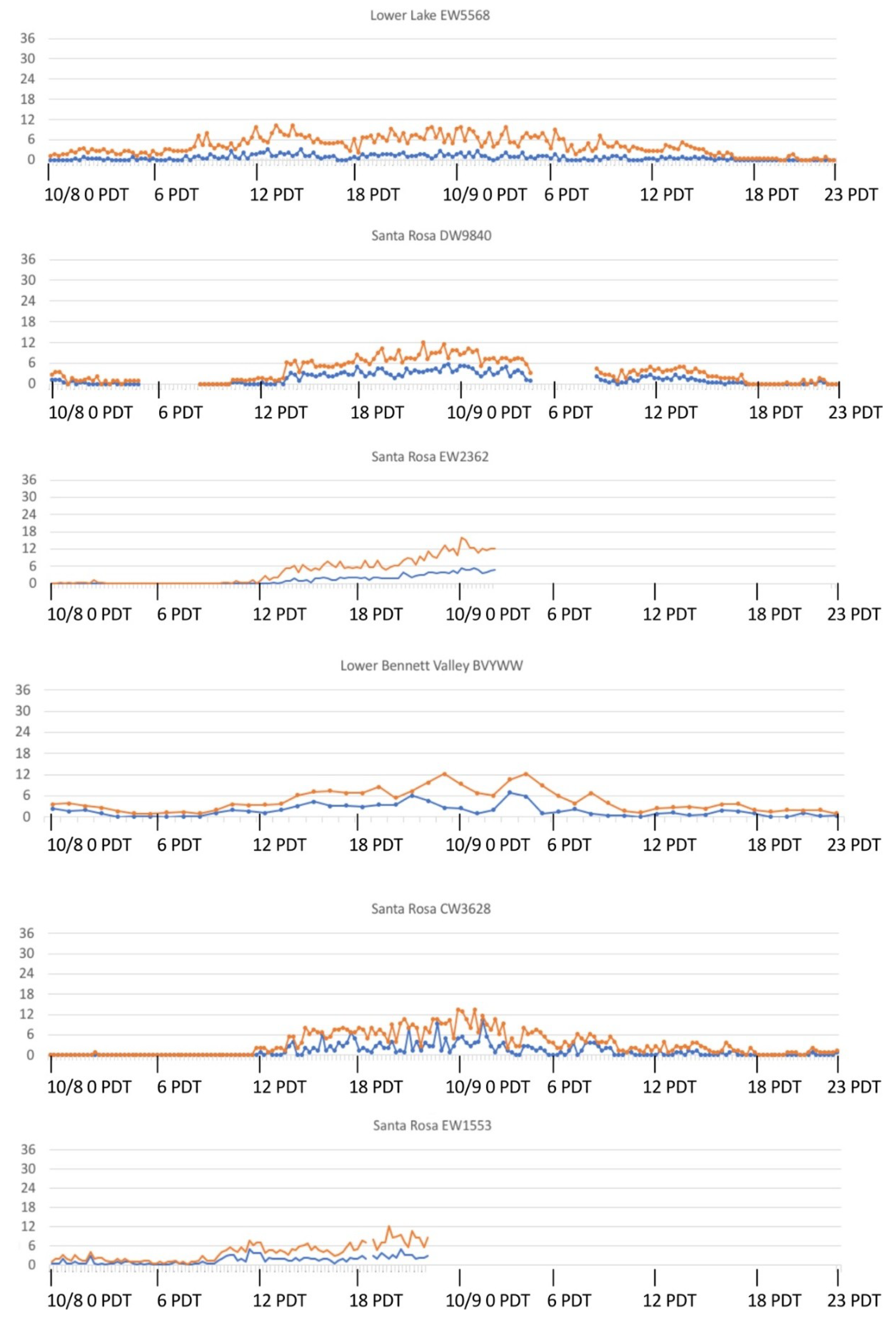
Figure 6.
Satellite active fire detection data of the Tubbs Fire. The “X” indicates the reported ignition location. Active fire detection data is available at http://activefiremaps.fs.fed.us.
Figure 6.
Satellite active fire detection data of the Tubbs Fire. The “X” indicates the reported ignition location. Active fire detection data is available at http://activefiremaps.fs.fed.us.

Figure 7.
The geographical extent of modeling domain 3.

Figure 8.
Simulated near-surface winds (8.5 m above ground level) on 8 October at 9:00 p.m. over the region shown in Figure 7. Wind speed arrows point downstream and are colored according to the color bar at right (in m/s). Imagery was produced with VAPOR (www.vapor.ucar.edu), a product of the Computational Information Systems Laboratory at the National Center for Atmospheric Research. In motion, as shown in Video S1, the field of arrows conveys changes in direction and strength of the Diablo winds.

Figure 9.
(a) Geographical extent and location of domain 4; (b) Simulated near-surface winds (8.5 m above ground level) on 8 October at 9:48 p.m. in domain 4. Wind speed arrows point downstream and are colored according to the color bar at right (in m/s). Vectors are shown every three grid points.
Figure 9.
(a) Geographical extent and location of domain 4; (b) Simulated near-surface winds (8.5 m above ground level) on 8 October at 9:48 p.m. in domain 4. Wind speed arrows point downstream and are colored according to the color bar at right (in m/s). Vectors are shown every three grid points.

Figure 10.
Retrospective research simulation of the Tubbs Fire using CAWFE. (a) VIIRS active fire detection data of the Tubbs Fire at 3:09 a.m. underlies simulated fire perimeter, the times of which are given by the legend. The red contour line corresponds to the time of the VIIRS observation. Terrain contour intervals are shown every 100 m; (b) The fire’s heat flux is show in the upper color bar (in W/m2). Wind speed arrows (in m/s) point downstream and are colored according to the color bar at right. Vectors are shown every three grid points.

Figure 11.
Cross-section through the retrospective research simulation of the Tubbs Fire (a) at 9:48 p.m. on 8 October, near the ignition time; and (b) at 3:03 a.m. on 9 October. Figures show an along-flow vertical cross section through the ignition (shown in (a) as a red X) while the contoured field is the simulated wind speed in the plane (in m/s), colored according to the color bar at right. Wind speed arrows (in m/s) point downstream and are shown every three grid points. The magenta box shows the area resembling a hydraulic jump at this time step, although speed maxima move through the cross section from right to left and the depth of the high-speed region dips over it.

Figure 12.
Simulation of the Tubbs fire using a forecast configuration. (a) Simulated extent at 11:25 p.m. on 8 October, where the pink line indicates the leading edge’s extent at the time of the model snapshot, as indicated in MODIS active fire detection data; (b) Similar to (a), at 3:09 a.m. on 9 October. In both frames, the fire’s heat flux is show in the lower color bar (in W/m2). Wind speed arrows (in m/s1) point downstream and are colored according to the upper color bar at right. Vectors are shown every three grid points.
© 2018 by the authors. Licensee MDPI, Basel, Switzerland. This article is an open access article distributed under the terms and conditions of the Creative Commons Attribution (CC BY) license (http://creativecommons.org/licenses/by/4.0/).
Share and Cite
MDPI and ACS Style
Coen, J.L.; Schroeder, W.; Quayle, B. The Generation and Forecast of Extreme Winds during the Origin and Progression of the 2017 Tubbs Fire. Atmosphere 2018, 9, 462. https://doi.org/10.3390/atmos9120462
AMA Style
Coen JL, Schroeder W, Quayle B. The Generation and Forecast of Extreme Winds during the Origin and Progression of the 2017 Tubbs Fire. Atmosphere. 2018; 9(12):462. https://doi.org/10.3390/atmos9120462
Chicago/Turabian StyleCoen, Janice L., Wilfrid Schroeder, and Brad Quayle. 2018. "The Generation and Forecast of Extreme Winds during the Origin and Progression of the 2017 Tubbs Fire" Atmosphere 9, no. 12: 462. https://doi.org/10.3390/atmos9120462
Note that from the first issue of 2016, this journal uses article numbers instead of page numbers. See further details here.