Improving Seasonal Prediction of East Asian Summer Rainfall Using NESM3.0: Preliminary Results


Abstract
1. Introduction
2. Model, Data and Initialization
2.1. The NESM3.0 Model
2.2. Major Improvement over the Early Version of the Model
2.3. The Data and Initialization
3. Performances on Predicted EASM Rainfall
4. Sensitivity of Each Modified Parameterization on Climatology and ENSO
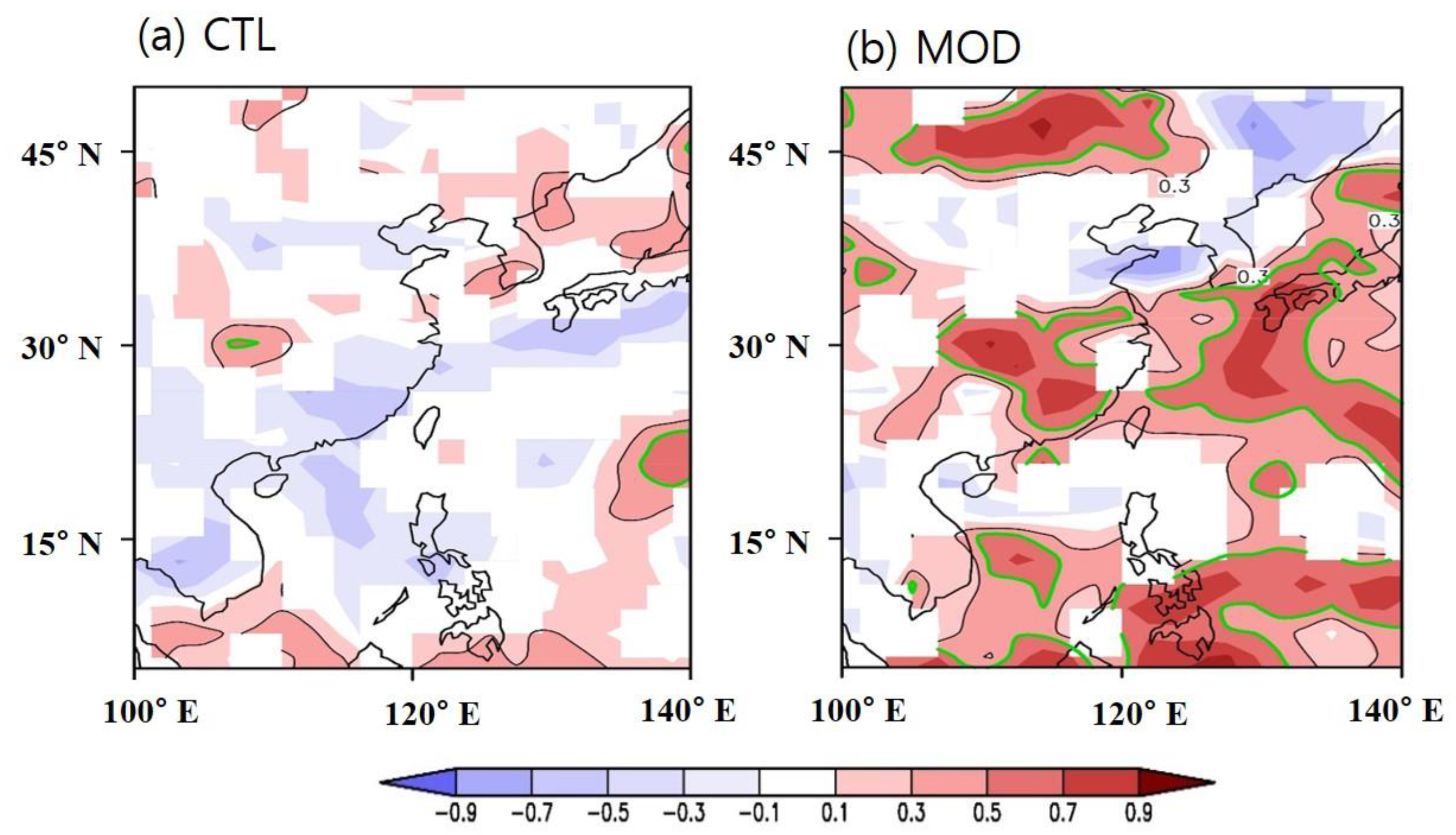
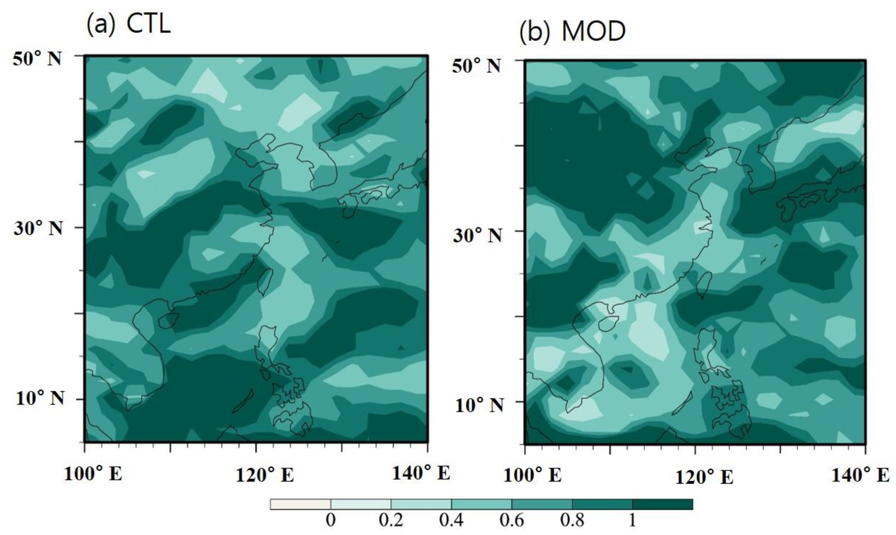
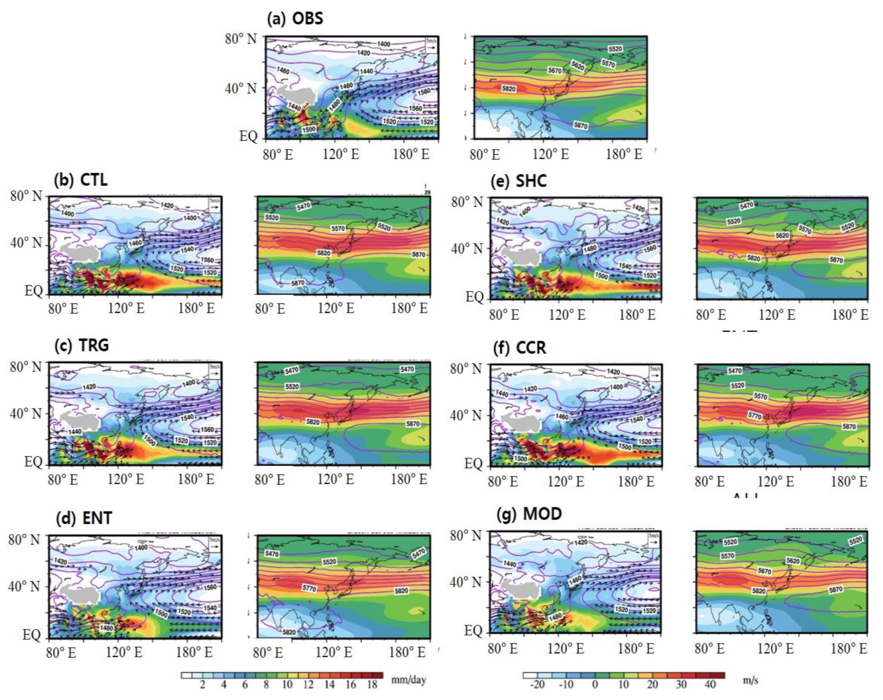
4.1. Climatology
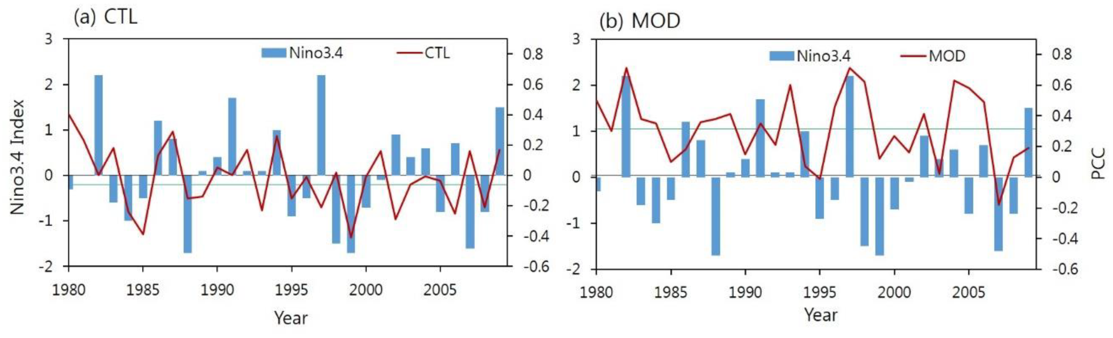
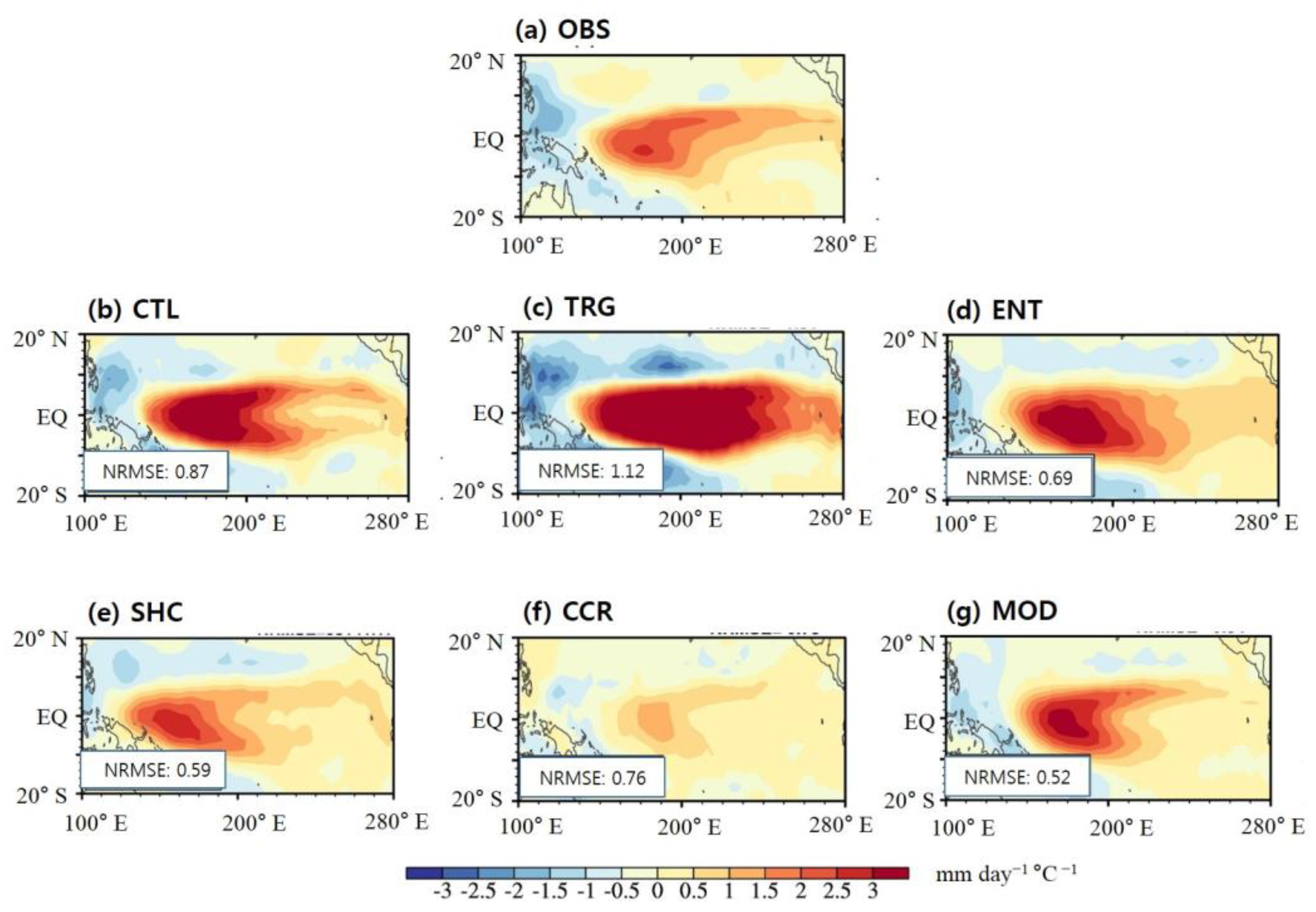
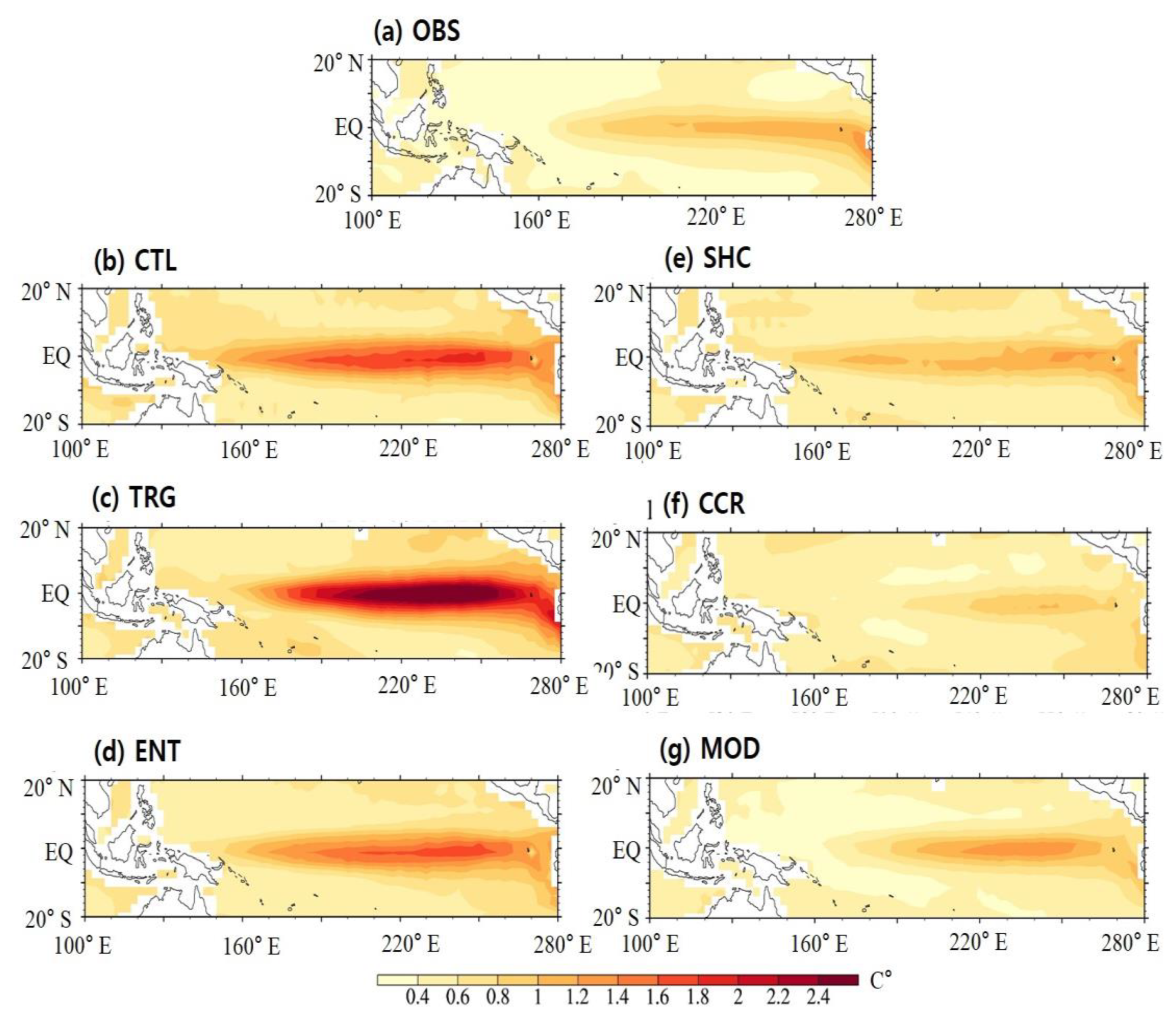
4.2. ENSO
5. Evaluation of Predicted Climatology and Major Modes of Variability
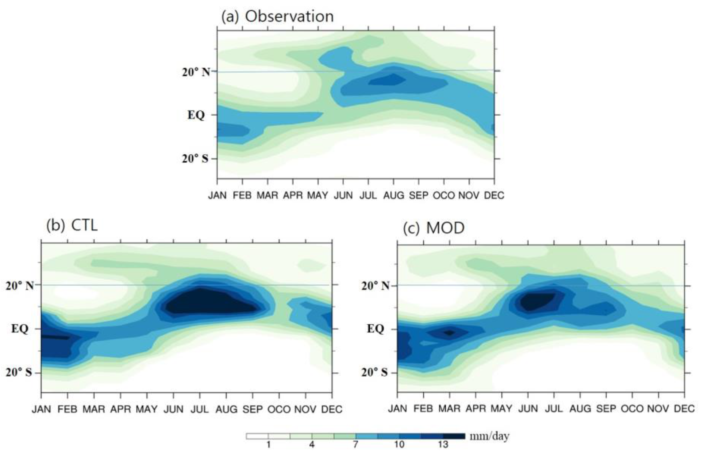
5.1. Seasonal Transition
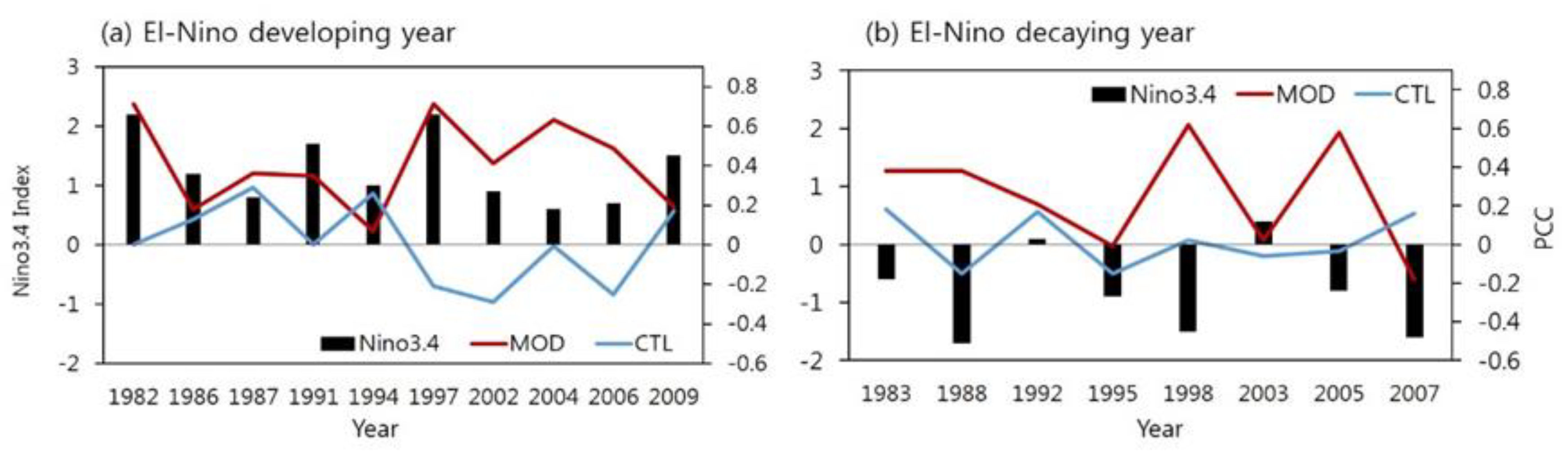
5.2. ENSO Prediction and EASM–ENSO Relationship
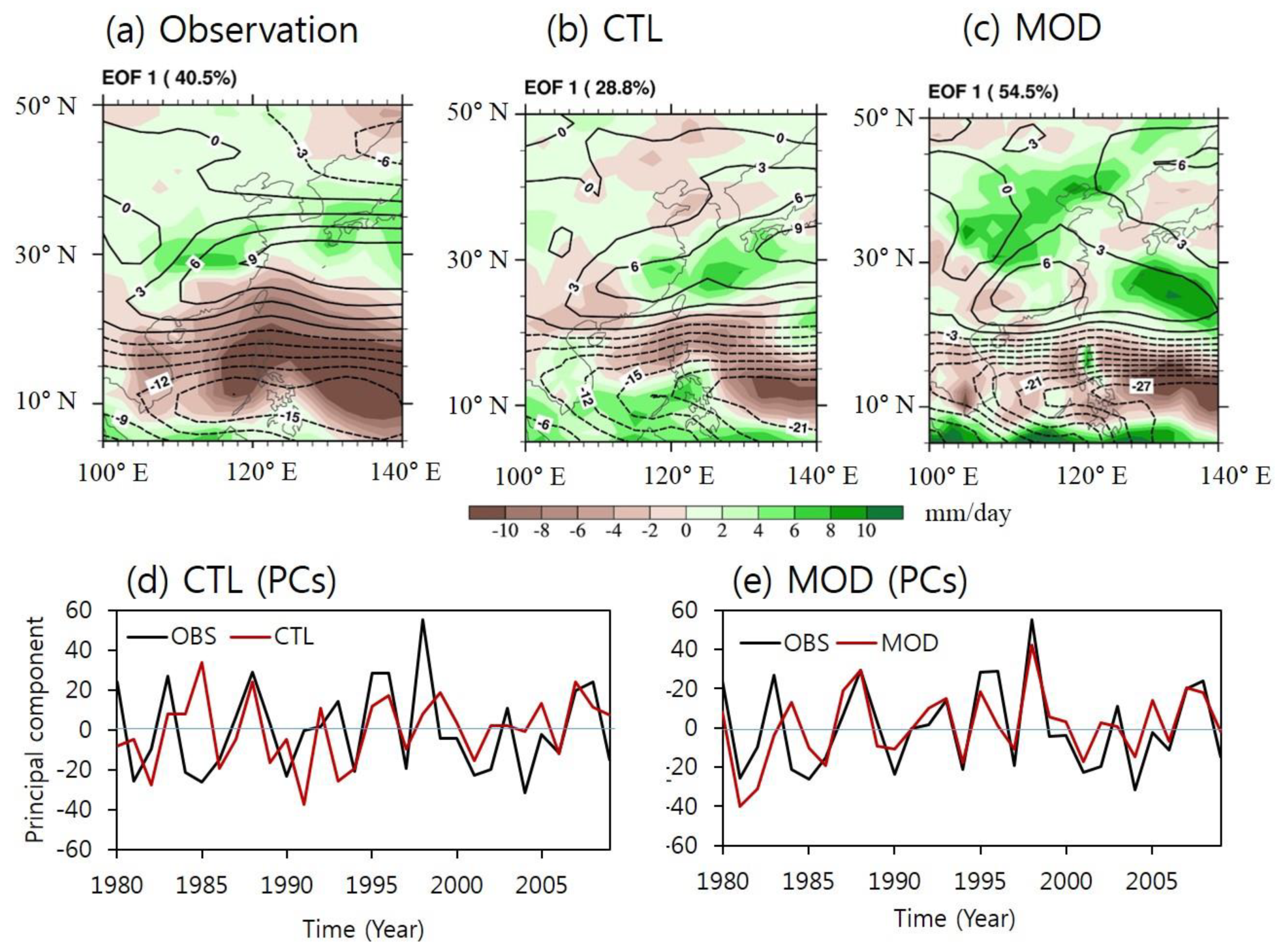
5.3. Major Modes of Interannual Variability of EASM
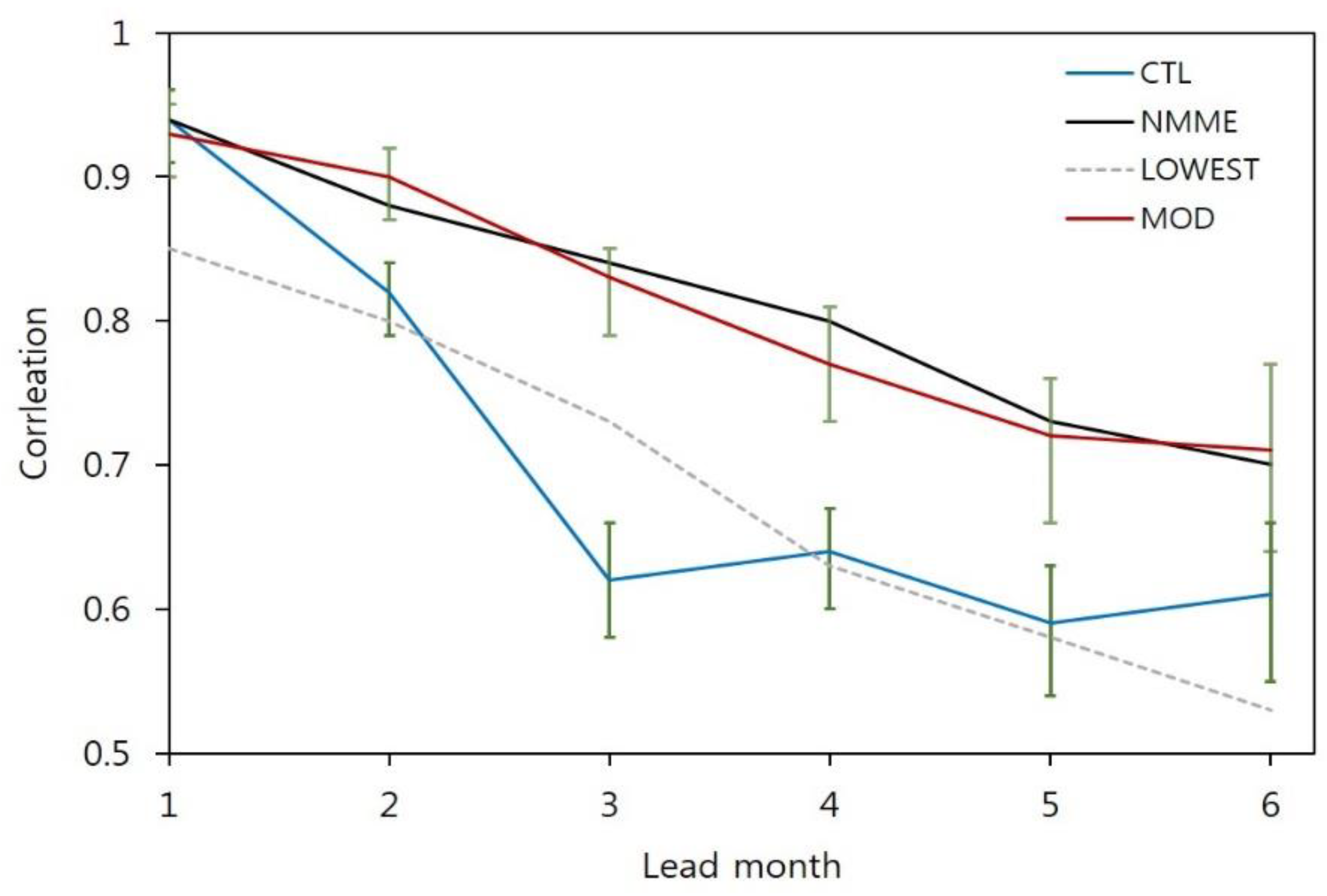
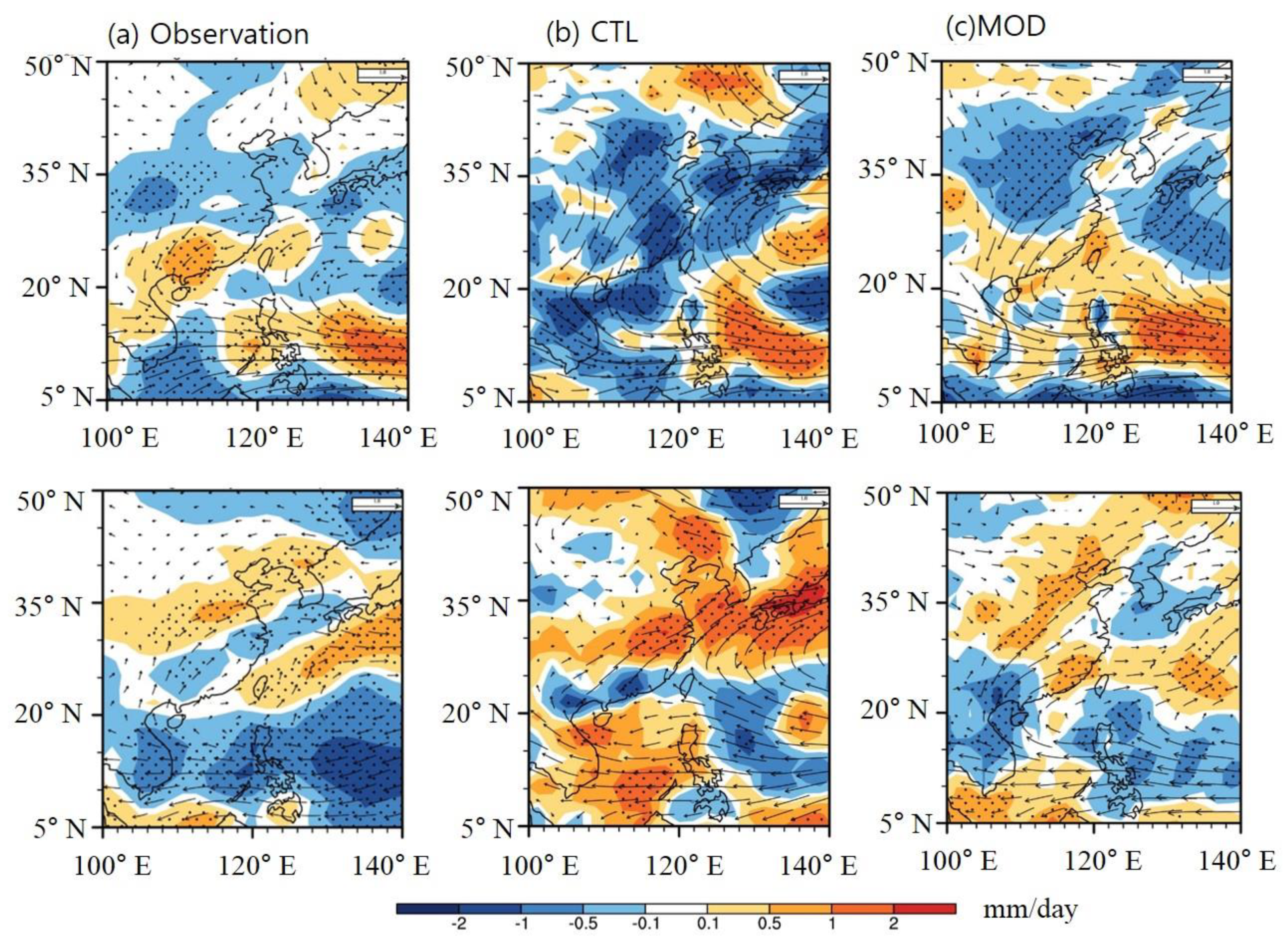
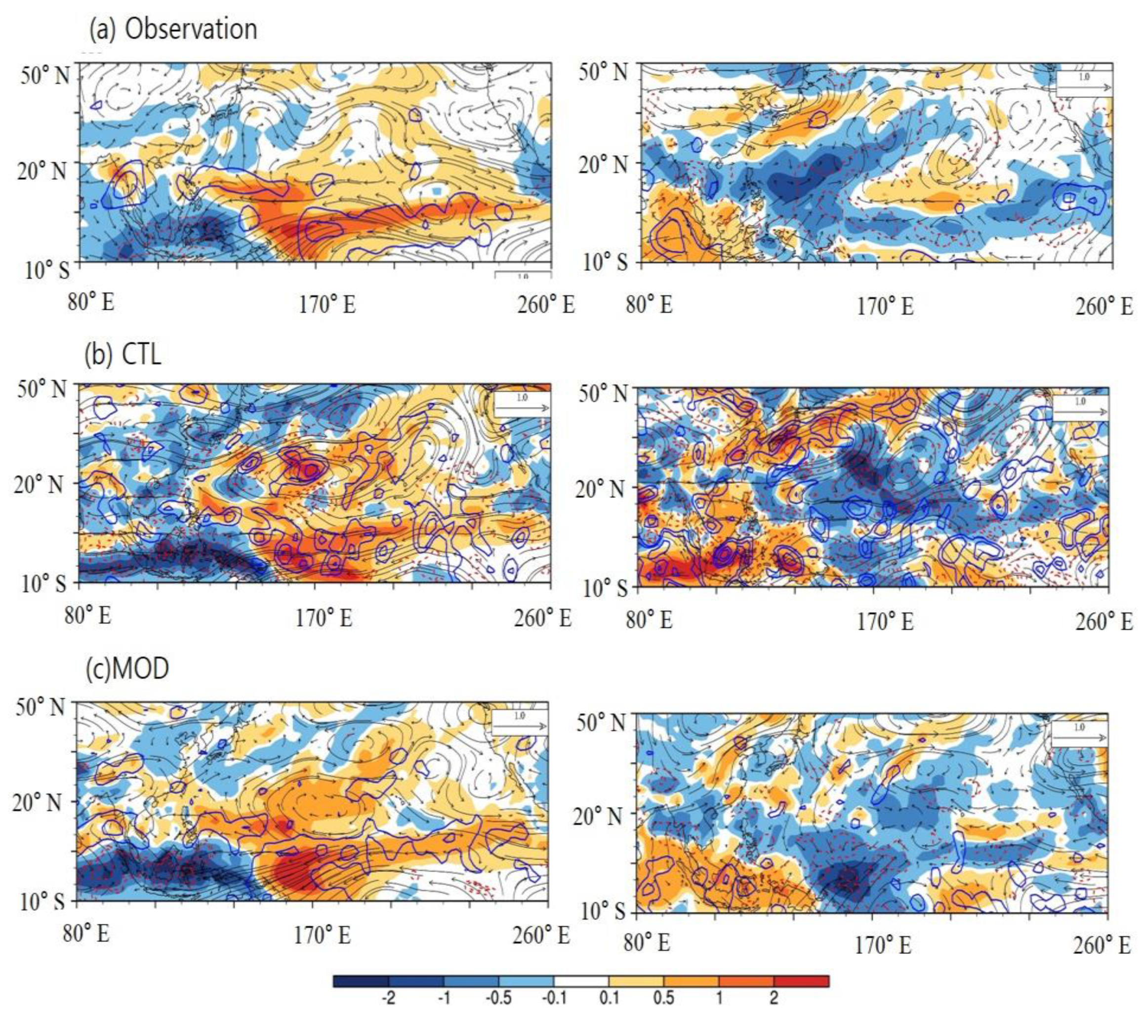
5.4. Prediction of EASM Circulation Index and Associated Rainfall Anomaly Pattern
6. Conclusions and Discussion
Author Contributions
Funding
Acknowledgments
Conflicts of Interest
References
- Kang, I.S.; Jin, K.; Wang, B.; Lau, K.M.; Shukla, J.; Krishnamurthy, V.; Schubert, S.; Wailser, D.; Stern, W.; Kitoh, A.; et al. Intercomparison of the climatological variations of Asian summer monsoon precipitation simulated by 10 GCMs. Clim. Dyn. 2002, 19, 383–395. [Google Scholar]
- Wang, B.; Zhang, Y.; Lu, M. Definition of South China Sea Monsoon Onset and Commencement of the East Asia Summer Monsoon. J. Clim. 2004, 17, 699–710. [Google Scholar] [CrossRef]
- Wang, B.; Ding, Q.; Fu, X.; Kang, I.-S.; Jin, K.; Shukla, J.; Doblas-Reyes, F. Fundamental challenge in simulation and prediction of summer monsoon rainfall. Geophys. Res. Lett. 2005, 32, L15711. [Google Scholar] [CrossRef]
- Tompkins, A.M.; Ortiz De Zarate, M.I.; Saurral, R.I.; Vera, C.; Saulo, C.; Merryfield, W.J.; Sigmond, M.; Lee, W.S.; Baehr, J.; Braun, A.; et al. The Climate-System Historical Forecast Project: Pro-viding Open Access to Seasonal Forecast Ensembles from Cen-ters around the Globe, B. Am. Meteorol. Soc. 2017, 98, 2293–2302. [Google Scholar] [CrossRef]
- Lee, J.-Y.; Wang, B.; Kang, I.S.; Shukla, J.; Kumar, A.; Kug, J.S.; Schemm, J.K.E.; Luo, J.J.; Yamagata, T.; Fu, X.; Alves, O. How are seasonal prediction skills related to models performance on mean state and annual cycle? Clim. Dyn. 2010, 35, 267–283. [Google Scholar] [CrossRef]
- Wang, B.; Lee, J.-Y.; Kang, I.-S.; Shukla, J.; Park, C.K.; Kumar, A.; Schemm, J.; Cocke, S.; Kug, J.S.; Luo, J.J.; et al. Advance and prospectus of seasonal prediction: As-sessment of the APCC/CliPAS 14-model ensemble retrospective seasonal prediction (1980–2004). Clim. Dyn. 2009, 33, 93–117. [Google Scholar] [CrossRef]
- Lee, D.Y.; Ahn, J.-B.; Yoo, J.-H. Enhancement of seasonal prediction of East Asian summer rainfall related to western tropical Pacific convection. Clim. Dyn. 2015, 45, 1025–1042. [Google Scholar] [CrossRef]
- Juan, L.; Wang, B.; Yang, Y.-M. A comprehensitve diagnostics metrics for evaluation and assessment of East Asian monsoon. J. Clim. 2018. submitted. [Google Scholar]
- Madec, G. NEMO Ocean Engine; Note du Pole de modélisation, Institut Pierre-Simon Laplace (IPSL): Paris, France, 2008. [Google Scholar]
- Hunke, E.C.; Lipscomb, W.H. CICE: The Los Alamos Sea Ice Model Documentation and Software User’s Manual; Version 4.0, LA-CC-06-012; Los Alamos National Laboratory: New Mexico, NM, USA, 2008.
- Valcke, S.; Craig, T.; Coquart, L. OASIS3-MCT User Guide(OASIS3-MCT 1.0); CERFACS: Toulouse, France, 2012. [Google Scholar]
- Cao, J.; Wang, B.; Yang, Y.-M.; Ma, L.; Li, J.; Sun, B.; Bao, Y.; He, J.; Zhou, X. The nuist earth system model (nesm) version 3: Description and preliminary evaluation. Geosci. Model Dev. Discuss. 2018, 1, 2975–2993. [Google Scholar] [CrossRef]
- Yang, Y.-M.; Wang, B. Improving MJO simulation by enhancing the interaction between boundary layer convergence and lower tropospheric heating. Clim. Dyn. 2018. [Google Scholar] [CrossRef]
- Yang, Y.-M.; Wang, B.; Lee, J.-Y. Mechanisms of northward propagation of boreal summer Intraseasonal Oscillation revealed by climate model experiments. Geophys. Res. Lett. 2018. submitted. [Google Scholar]
- Stevens, B.; Giorgetta, M.; Esch, M.; Mauritsen, T.; Crueger, T.; Rast, S.; Salzmann, M.; Schmidt, H.; Bader, J.; Block, K.; et al. The Atmospheric Component of the MPI-M Earth System Model: ECHAM6. J. Adv. Model. Earth Syst. 2017, 5, 146–172. [Google Scholar] [CrossRef]
- Tiedtke, M. A comprehensive mass flux scheme for cumulus parameterization in large-scale models. Mon. Weather Rev. 1989, 117, 1779–1800. [Google Scholar] [CrossRef]
- Nordeng, T.E. Extended Versions of the Convective Parametrization Scheme at ECMWF and Their Impact on the Mean and Transient Activity of the Model in the Tropics; European Centre for Medium-Range Weather Forecasts: Reading, UK, 1994. [Google Scholar]
- Wen, M.; Yang, S.; Kumar, A.; Zhang, P. An Analysis of the Large-Scale Climate Anomalies Associated with the Snowstorms Affecting China in January 2008. Mon. Weather Rev. 2009, 137, 1111–1131. [Google Scholar] [CrossRef]
- Yang, S.; Smith, E.A. Convective-stratiform precipitation variability at seasonal scale from 8 yr of trmm observations: Implications for multiple modes of diurnal variability. J. Clim. 2008, 21, 4087–4114. [Google Scholar] [CrossRef]
- Tokioka, T.; Yamazaki, K.; Kitoh, A.; Ose, T. The equatorial 30-60 day oscillation and the Arakawa-Schubert penetrative cumulus parameterization. J. Meteorol. Soc. Jpn. 1988, 66, 883–901. [Google Scholar]
- Kim, D.; Kang, I.-S. A bulk mass flux convection scheme for climate model: Description and moisture sensitivity. Clim. Dyn. 2012, 38, 411–429. [Google Scholar] [CrossRef]
- Kanamitsu, M.; Ebisuzaki, W.; Woollen, J.; Yang, S.-K.; Hnilo, J.J.; Fiorino, M.; Potter, G.L. NCEP–DOE AMIP-II Reanalysis (R.-2). Bull. Am. Meteorol. Soc. 2002, 83, 1631–1643. [Google Scholar] [CrossRef]
- Adler, R.F.; Huffman, G.J.; Chang, A.; Ferraro, R.; Xie, P.P.; Janowiak, J.; Rudolf, B.; Schneider, U.; Curtis, S.; Bolvin, D.; Gruber, A. The Version-2 Global Precipitation Climatology Project (GPCP) Monthly Precipitation Analysis (1979–Present). J. Hydrometeorol. 2003, 4, 1147–1167. [Google Scholar] [CrossRef]
- Huang, B.; Thorne, P.W.; Smith, T.M.; Liu, W.; Lawrimore, J.; Banzon, V.F.; Zhang, H.M.; Peterson, T.C.; Menne, M. Further Exploring and Quantifying Uncertainties for Extended Reconstructed Sea Surface Temperature (ERSST) Version 4 (v4). J. Clim. 2015, 29, 3119–3142. [Google Scholar] [CrossRef]
- Kang, I.S.; Jang, P.H.; Almazroui, M. Examination of multi-perturbation methods for ensemble prediction of the MJO during boreal summer. Clim. Dyn. 2014, 42, 2627–2637. [Google Scholar] [CrossRef]
- George, S.E. Predictability and skill of boreal winter forecasts made with the ECMWF seasonal forecast system II. Q. J. R. Meteorol. Soc. 2006, 132, 2031–2053. [Google Scholar] [CrossRef]
- Zhou, T.-J.; Yu, R.-C. Atmospheric water vapor transport associated with typical anomalous summer rainfall patterns in China. J. Geophys. Res. Atmos 2005, 110, D8. [Google Scholar] [CrossRef]
- Zhou, W.; Chan, J.C.L.; Chen, W.; Ling, J.; Pinto, J.G.; Shao, Y. Synoptic-Scale Controls of Persistent Low Temperature and Icy Weather over Southern China in January 2008. Mon. Weather Rev. 2009, 137, 3978–3991. [Google Scholar] [CrossRef]
- Wang, B.; Xiang, B.; Lee, J.-Y. Subtropical High predictability establishes a promising way for monsoon and tropical storm predictions. Proc. Natl. Acad. Sci. 2013, 110, 2718–2722. [Google Scholar] [CrossRef]
- Kim, D.; Jang, Y.S.; Kim, D.H.; Kim, Y.H.; Watanabe, M.; Jin, F.F.; Kug, J.S. El Niño–Southern Oscillation sensitivity to cumulus entrainment in a coupled general circulation model. J. Geophys. Res. 2011, 116, D22112. [Google Scholar] [CrossRef]
- Watanabe, M.; Chikira, M.; Imada, Y.; Kimoto, M. Convective control of ENSO simulated in MIROC. J. Clim. 2011, 24, 543–562. [Google Scholar] [CrossRef]
- Wang, B.; Li, J.; He, Q. Variable and robust East Asian monsoon rainfall response to El Niño over the past 60 years (1957–2016). Adv. Atmos Sci. 2017, 34, 1235–1248. [Google Scholar] [CrossRef]
- Huang, R.; Wu, Y. The influence of ENSO on the summer climate change in China and its mechanism. Adv. Atmos Sci. 1989, 6, 21–32. [Google Scholar]
- Kirtman, B.P.; Min, D.; Infanti, J.M.; Kinter, J.L., III; Paolino, D.A.; Zhang, Q.; van den Dool, H.; Saha, S.; Mendez, M.P.; Becker, E. The North American Multi-Model Ensemble (NMME): Phase-1 Seasonal to Interannual Prediction, Phase-2 Toward Developing Intra-Seasonal Prediction. Bull. Am. Meteorol. Soc 2014, 95, 585–601. [Google Scholar] [CrossRef]
- Wang, B. The vertical structure and development of the ENSO anomaly mode during 1979–1989. J. Atmos Sci. 1992, 49, 698–712. [Google Scholar] [CrossRef]
- Fan, K.; Liu, Y.; Chen, H. Improving the prediction of the East Asian summer monsoon: New approaches. Weather Forecast. 2012, 27, 1017–1030. [Google Scholar] [CrossRef]
- Wang, B.; Wu, Z.; Li, J.; Liu, J.; Chang, C.P.; Ding, Y.; Wu, G. How to measure the strength of the East Asian summer monsoon. J. Clim. 2008, 21, 4449–4463. [Google Scholar] [CrossRef]


© 2018 by the authors. Licensee MDPI, Basel, Switzerland. This article is an open access article distributed under the terms and conditions of the Creative Commons Attribution (CC BY) license (http://creativecommons.org/licenses/by/4.0/).
Share and Cite
Yang, Y.-M.; Wang, B.; Li, J. Improving Seasonal Prediction of East Asian Summer Rainfall Using NESM3.0: Preliminary Results. Atmosphere 2018, 9, 487. https://doi.org/10.3390/atmos9120487
Yang Y-M, Wang B, Li J. Improving Seasonal Prediction of East Asian Summer Rainfall Using NESM3.0: Preliminary Results. Atmosphere. 2018; 9(12):487. https://doi.org/10.3390/atmos9120487
Chicago/Turabian StyleYang, Young-Min, Bin Wang, and Juan Li. 2018. "Improving Seasonal Prediction of East Asian Summer Rainfall Using NESM3.0: Preliminary Results" Atmosphere 9, no. 12: 487. https://doi.org/10.3390/atmos9120487
APA StyleYang, Y.-M., Wang, B., & Li, J. (2018). Improving Seasonal Prediction of East Asian Summer Rainfall Using NESM3.0: Preliminary Results. Atmosphere, 9(12), 487. https://doi.org/10.3390/atmos9120487