Evaluation of Analysis by Cross-Validation. Part I: Using Verification Metrics


Air Quality Research Division, Environment and Climate Change Canada, 2121 Transcanada Highway, Dorval, QC H9P 1J3, Canada
*
Author to whom correspondence should be addressed.
Atmosphere 2018, 9(3), 86; https://doi.org/10.3390/atmos9030086
Submission received: 5 September 2017
/
Revised: 20 February 2018
/
Accepted: 24 February 2018
/
Published: 27 February 2018
(This article belongs to the Special Issue Air Quality Monitoring and Forecasting)
Abstract
:We examine how passive and active observations are useful to evaluate an air quality analysis. By leaving out observations from the analysis, we form passive observations, and the observations used in the analysis are called active observations. We evaluated the surface air quality analysis of O3 and PM2.5 against passive and active observations using standard model verification metrics such as bias, fractional bias, fraction of correct within a factor of 2, correlation and variance. The results show that verification of analyses against active observations always give an overestimation of the correlation and an underestimation of the variance. Evaluation against passive or any independent observations display a minimum of variance and maximum of correlation as we vary the observation weight, thus providing a mean to obtain the optimal observation weight. For the time and dates considered, the correlation between (independent) observations and the model is 0.55 for O3 and 0.3 for PM2.5 and for the analysis, with optimal observation weight, increases to 0.74 for O3 and 0.54 for PM2.5. We show that bias can be a misleading measure of evaluation and recommend the use of a fractional bias such as the modified normalized mean bias (MNMB). An evaluation of the model bias and variance as a function of model values also show a clear linear dependence with the model values for both O3 and PM2.5.
1. Introduction
Since 2003, Environment and Climate Change Canada (ECCC) has been producing hourly surface analyses of pollutants covering North America [1,2] which became operational products in February 2013 [3]. The analyses are produced using an optimum interpolation scheme that combines the operational air quality forecast model GEM-MACH output [4] (CHRONOS model output was used prior to 2010 [5]) with real-time hourly observations of O3, PM2.5, PM10, NO2, and SO2 from the AirNow gateway with additional observations from Canada. As those surface analyses are not used to initialize an air quality model, it raises the issue on how to evaluate them. We conduct routine evaluations using the same set of observations as those used to produce the analysis. Once in a while, when there is a change in the system, a more thorough evaluation is conducted where we leave out a certain fraction of the observations and use them as independent observations, a process known as cross-validation. Observations used in producing the analysis are called active observations while those not used for evaluation are passive observations. Cross-validation is used to validate any model that depends on data. In air quality applications it has been used, for example, for mapping and exposure models [6,7,8]. The purpose of this two-part paper is to examine the relative merit of using active or passive observations (or independent observations in general) viewed from different evaluation metrics, but also to develop, in the second part, a mathematical framework to estimate the analysis error, and in doing so, to improve the analysis.
The evaluation of an analysis is important, even in the case where it is used to initialize an air quality forecast model, since the evaluation of the resulting air quality forecast may not be a good measure of the quality of the analysis. In air quality forecasting, the forecast error growth is small, depicts little sensitivity to initial conditions and is in fact more sensitive to numerous modeling errors such as: photochemistry, clouds, meteorology, boundary conditions and emissions just to name a few [9,10,11,12,13]. Furthermore, chemical species that are observed are incomplete compared to species needed to initialize an air quality model, incomplete in terms of the number of species observed as well as in their kind [9,11,13,14]. Only a fraction of the observed species (either of secondary or primary pollutants) are usable for data assimilation; important chemical mechanisms are left completely unobserved and for aerosols, information on size distribution is quite limited and almost nonexistent when it comes to speciation [9,13]. In addition, the observational coverage is limited to the surface or to total column measurements which, up until now, were available at one or two local times per day. There are thus many assumptions to be made from an analysis to a proper 3D initial chemical condition and surface emission correction and its subsequent impact on the air quality forecast. These considerations warrant an independent evaluation of the quality of the analysis on its own [15].
Evaluating an analysis with observations is quite different from evaluating a model with observations, since analyses are created from observations. From a statistical point of view, the observation and analysis cannot be considered independent. However, let us assume that observation errors are spatially uncorrelated. Then, since the passive and active observation sites are never collocated, then the errors from passive observations are uncorrelated with errors of active observations (i.e., observations that are used for the analysis). Furthermore, since the modelling errors are usually assumed to be uncorrelated with observation errors, then it is also uncorrelated with the analysis errors. Cross-validation thus offers a means to evaluate analyses with statistically independent (passive) observations [16].
In part one of this paper, we evaluate the relative merit of passive and active observations in the evaluation of analyses using standard metrics used for model evaluation. We show how and when the use of active observations can be misleading and that passive observations can provide a means to identify optimal analyses. Our examples show that optimal analyses, at the independent observation sites, have much smaller biases than the model biases and increase the correlation coefficient by nearly a factor of 2.
The paper is thus organized as follows. First we present the analysis scheme we will be using, as well as the cross-validation design, the evaluation metrics and the configuration of the experiments. Then in Section 3, we assess the quality of the analyses in both active and passive observation spaces using standard air quality evaluation metrics, identify some pitfalls of some metrics and advocate using active observations. Conclusions are presented in Section 4.
2. Experimental Design
2.1. Design of the Objective Analysis Solver
In optimum interpolation there is no use of an explicit interpolation observation operator. The correlation between a pair of locations, either from two observation sites or from an observation site to a model grid point, is computed as a function of distance using a prescribed correlation function. The observation operator is in effect a delta function applied over a continuous spatial domain [17].
In this study we interpolate the gridded analysis field to observation locations, using bilinear interpolation, to compute residuals such as observation-minus-analysis. Thus there can be a discrepancy between the observation operator used to generate the analysis, i.e., delta functions, and the observation operator used to interpolate the analysis field at the observation location, i.e., bilinear interpolation. To eliminate this discrepancy in observation operators we have revised the optimum interpolation scheme to use explicitly the same bilinear interpolation in handling the error covariance. We will give details below.
As in the operational optimum interpolation, the inversion of the innovation covariance matrix for the analysis solver is done using Choleski decomposition on the full matrix. The number of observations to be processed per analysis being of the order of a thousand or less, there was no need for computational simplification for large number of observations by using either data selection [18] or compact support correlation functions [17,19]. Thus, the analysis scheme used in this study computes explicitly the gain matrix as,
where is a bilinear interpolation operator, is the prescribed background error covariance and is the prescribed observation error covariance. The tilde () emphasizes that these are prescribed, potentially suboptimal, quantities.
The computational demand of the Kalman gain was kept low by computing the background error correlation function only at model grid points needed for the bilinear interpolation. For example, to calculate the correlation between a pair of observations requires the computation of correlation between four points surrounding observation 1 (needed for the bilinear interpolation) and the other four points surrounding observation 2, thus forming a correlation matrix between the target model grid points. Then we calculate which gives the correlation between two observation sites. This procedure is generalized for the observations needed for the analysis. Equation (1) also involves the computation of that we compute as a set of representers (i.e., columns of ), each being a 2D field that maps the background error covariance in model space with a single observation location, using again the bilinear interpolation approach to get a single interpolated representor for each observation location. By doing so we keep the consistency between the observation operators used for interpolation of a field and the observation operator used to manipulate matrices.
2.2. Cross-Validation
Cross-validation is a technique to evaluate an analysis (or in general any model that depends on observations) by partitioning the original observation data set into a training set, used to create the analysis, and an independent (or passive) set, used to evaluate the analysis. The most common cross-validation designs are: the k-fold cross-validation, where the original observation data set is partitioned into k equal size subsamples and the leave-one-out cross-validation, where N subsamples are created, each with one different observation set aside for the evaluation while the other observations are used in producing the analysis. The cross-validation is then repeated with all the different sets until all observations have been used for evaluation. Clearly, there are k analyses computed in the k-fold cross-validation and N in the leave-one-out cross-validation, which is being computationally demanding when N is large. The main disadvantage of the k-fold cross-validation is that the analyses being evaluated uses a smaller number of observations (actually ) than the original observation data set, whereas the leave-one-out cross-validation evaluates analysis that uses nearly the same number of observations (actually ) as the original observation data set. This actually matters with the k-fold cross-validation if we need an estimate of the analysis error variance (or any other second moments) as the analysis error variance depends on the number of observations used.
Let be a vector that contains the jth set of observations used for evaluation, and let be a vector of analysis value interpolated at the verification observation locations of and where the analysis used all observations except those in (the index in parenthesis, i.e., , indicates all sets except the set j). It is customary in cross-validation literature (e.g., [20]) to construct a mean square error cost function, often denoted by CV,
that represents a misfit quadratic error of the model - in our case the analysis. Different model can be compared and selected from which the CV value is smallest. Likewise, a tunable parameter in can be obtained by minimizing the cost function CV with respect to that parameter. As we shall discuss later in this paper, in Section 4 and onwards, the bias of needs to be removed from the cost function in order to estimate the input error covariance parameters.
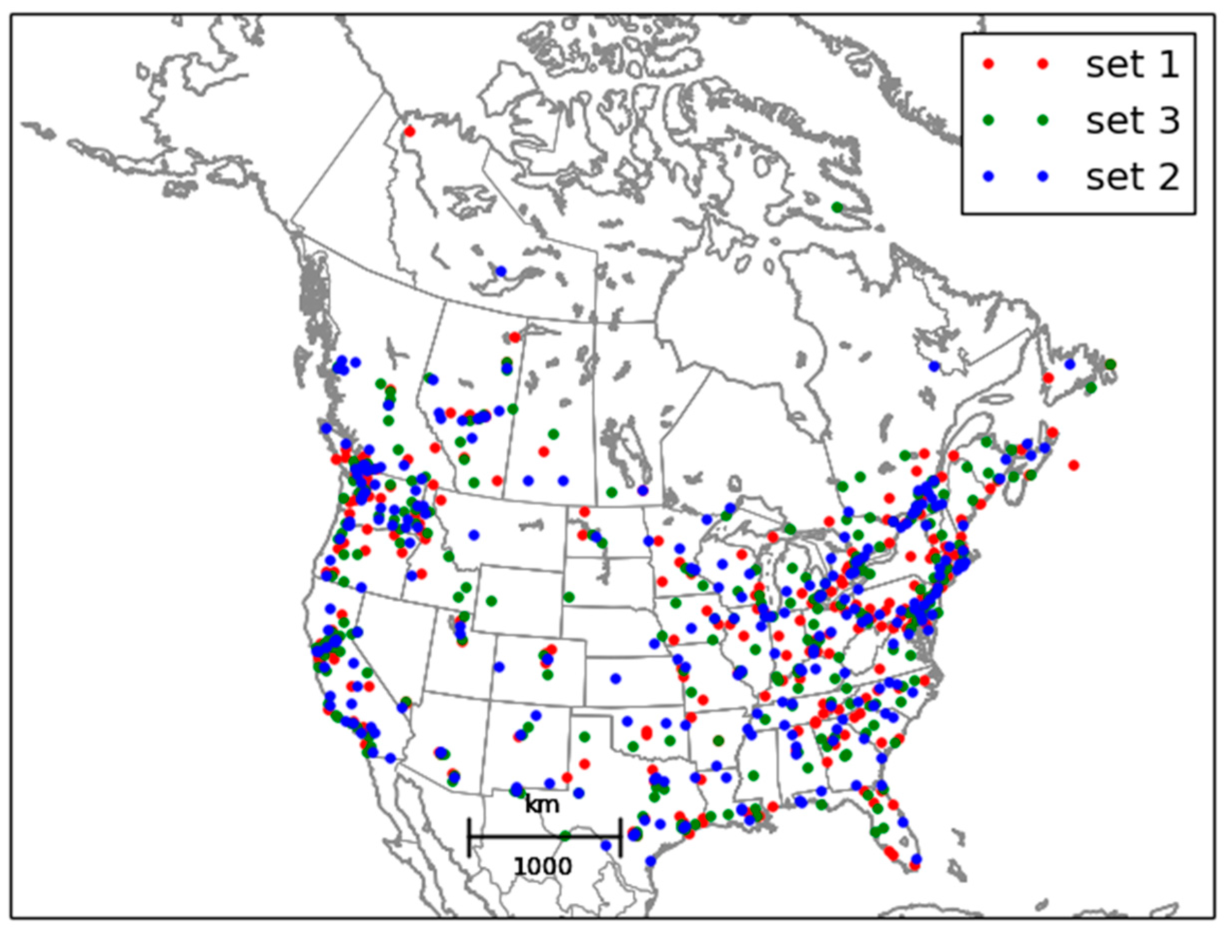
In applications and thus in all experiments that follow, the analyses and verification against passive observations are made only with a set of observations that have passed a quality control. The quality control is nearly identical to the quality control used for the operational implementation of the analysis of surface pollutants at ECCC (see supplementary material in Robichaud et al. [3]). It consists in discarding observations that report a negative value, or whose value exceeds a certain unrealistic threshold set to 300 ppbv for ozone (300 μg/m3 for PM2.5). Observations are also discarded based on innovations (or observed-minus-background values) when, for ozone, they exceed 50 ppbv (100 μg/m3 for PM2.5) in absolute value. The quality-controlled observations are then separated into three sets of observations of equal numbers, i.e., a 3-fold cross-validation procedure, as illustrated in Figure 1.
The selection into three sets is made by station ID number, selecting on a regular basis each fourth station, starting with station 1 for the first set, station 2 for the second set and station 3 for the third set, and resulting in locally spatially random distribution of each sets of stations. The cross-validation is then made by leaving one set out of the three sets, and using the remaining two sets to produce the analysis.
2.3. Verification Metrics
We will evaluate the analyses against passive and active observations with the following standard evaluation metrics used for air quality models [21,22,23,24]; the bias, the modified normalized mean bias (MNMB), the fraction of correct within a factor of 2 (FC2), the variance (var(O − A)) and the correlation coefficient (), where the statistics is computed over time t for each station, and then the resulting metric is averaged over all the verifying station i,
where is the observed value at time at the station i, is the analysis at time interpolated at the location of the station i, is the total number of time sample per station, is the total number of stations (in the sample or over the domain), and the overbar denotes the time average. The bias and the MNMB are metrics of the first moment that have distinctive properties. The bias gives a representative measure of the systematic discrepancy between analyzed and observed values over the whole set of observations used for verification. However, since atmospheric constituents exhibit a range of values that can vary in time and space, and different constituents have different range of values and may as well be expressed with different units, a relative error measure such as the MNMB is often preferred [24]. The MNMB is a dimensionless quantity that falls in the range . The factor of 2 is introduced so to give a % error interpretation to the MNMB. This metric has the additional advantage of treating over- and under-estimation in a symmetric way [24]. However, the MNMB is relatively insensitive to relatively large discrepancies between analysis (or model) values and observed values, that is when its values are close to +2 (200%) or −2 (−200%) [23].
The fraction of correction within a factor of 2 (FC2) is a measure of reliability. It is based on counts and has the distinctive advantage that it is insensitive to outliers. It is worth mentioning that it accounts both high values outliers and also low values outliers that is a unique property of this metric [22]. The FC2 metric is also symmetric with respect to permutation of A and O, it is also dimensionless and its values must lie between 0 and 1. Our experience with this metric indicates that it is relatively insentive for relatively good agreement between analysis and observed values.
The variance, var(O − A), and the correlation coefficient are metrics that depend on the spread of the discrepancy between analysis and observed values. The variance is not a dimensionless metric. It gives a representative measure of the spread of the discrepancy between analyses and observations and is not sensitive to systematic errors. As we will show in Section 4 and also shown in Marseille et al. [16], var(O − A) with passive observations has the distinct advantage of providing a measure of the true analysis error variance (i.e., the error with respect to the truth) and var(O − A) can be considered as a cross-validation cost function CV, Equation (2), with debiased (O − A) increments. As for any second moment metric, var(O − A) is sensitive to outliers; they must be removed, and this is done by gross check of the , as explained in the previous subsection Section 2.2. Finally, the correlation coefficient is a dimensionless quantity that lies in the range [−1, +1]. It is also invariant to shifts in the mean (i.e., not sensitive to systematic errors), and multiplicative rescaling of either analysis or observations. The correlation is also relatively insensitive to improvement when the correlation is close to 1 or −1.
2.4. Description of the Ensemble of Analyses and Their Verification Statistics
A series of hourly analyses of O3 and PM2.5 at 21 UTC for a period of 60 days (14 June to 12 August 2014) were performed with given input error statistics using the operational model GEM-MACH and the real-time AirNow observations as described in the introduction and with quality controlled observations (see Section 2.2 above). In all experiments, the observation and background error variances, and , used in the analysis are uniform. The prescribed observation error and background error covariances are given as , , where the correlation model is a homogeneous isotropic second-order autoregressive model with a correlation length obtained by maximum likelihood, as in Ménard et al. [17]. Note that aside from quality control, that ends up rejecting some observations, the analysis uses the observation values and model realizations as is, with no bias correction.
We repeat the series of 60 day analyses for different observation and background error variances chosen in such a way that their sum is equal to but with different ratios of error variances . We perform the series of analyses over a wide range of ratios in the interval , thus creating on one end analyses with very large observation weights, i.e., , such that the analysis interpolated at the active observation sites tend to match the observed value, and on the other end, with , creating analyses with very small observation weight producing analyses that are very close to the background (model) state.
The condition , called the innovation variance consistency, is an important constraint that is useful for the estimation of the true error statistics [25]. Indeed, the stronger condition for the full covariance matrices, the innovation covariance consistency criterion, takes the form: , where represents the mean over an ensemble of realizations, is the interpolation from model grid to the observation location (or observation operator). It is one of the two necessary and sufficient condition to obtain the true error covariance statistics (in observation space) [25,26].
As explained in Section 2.3 above, the verification metrics are first calculated over 60 days for a given hour and for each station. Then the metric is averaged over all the verifying stations, resulting in one value of the metric for each hour of the day. Here, however, we computed the metrics for 21 UTC only. If is the total number of stations, the statistics over one of the 3-fold subset then involves an average of the metric over passive stations. Doing this for all three subsets, and taking the average of the subsets’ results, is equivalent to taking the average of the metric over all stations. In the results that will be presented in the following sections, we always present the average metric over the three passive subsets so that, in the end, the sample size of the passive observation experiments and of the active observation experiments are equal and thus can be presented side by side on the same graphic.
3. Verification against Passive and Active Observations
In this series of experiments, analyses of O3 and PM2.5 were produced using a fixed homogeneous isotropic correlation function, where the correlation length was obtained by maximum likelihood using a second-order auto-regressive model and error variances computed using a local Hollingsworth-Lönnberg fit [17]. A correlation length of 124 km was obtained for O3 and of 196 km for PM2.5. Our correlation length is defined from the curvature at the origin as in Daley [27] and is different from the length-scale parameter of the correlation model (see Ménard et al. [17] for a discussion of these issues). We did a series of 60-days analyses for different values of and but such that their sum respects the innovation variance consistency, , an important condition for an optimal analysis [25], as explained in Section 2.4. This is the experimental procedure that has been used to generate the Figure 2, Figure 3, Figure 4, Figure 5, Figure 6 and Figure 7. The results are shown for a wide range of variance ratios from to in Figure 2, Figure 3, Figure 4, Figure 5 and Figure 7 in particular. Note that corresponds to a very large observation weight while correspond to very small observation weight.
The using passive observations (red curve with circles) and active observations (black curve with squares) is presented in Figure 2 for O3 (left panel) and PM2.5 (right panel). The solid blue line represents , the variance of observation-minus-model, i.e., prior to an analysis. As mentioned in Section 2.4, in the cross-validation experiments we averaged the verification metric over the 3-fold subsets so that, in effect, the total number of observations that end up being used for verification is , the total number of stations. We thus argue that the verification sampling error for the cross-validation experiments (red curve) is the same as for the active observations using the full analysis (i.e., analysis using the total number of stations; black curve). In addition, note that from Figure 1 the station sampling strategy gives rise to spatially random selection of stations, so that the individual metric on each set should be comparable. Furthermore, there is roughly 1300 quality controlled O3 observations over the domain and 750 PM2.5 quality controlled observations, each with 60 time samples or less. To give some qualitative idea of the sampling error, the different metric values for the individual 3-fold sets are presented in the Supplementary Material Figures S1 and S2, where we can see that for and the metric values for the individual sets are nearly indistinguishable from the means of the 3-subset.
The difference between the verification against passive observations in cross-validation analyses (red curve) and the verification against active observations using full analyses (black curve) can be attributed to two effects: (1) the analysis used in the cross-validation uses 2/3rd of the total number of observations and thus the analysis error has larger variance than analyses using all observations, (2) since the analysis error variance has typically a local minimum at the individual active observation sites and increases away from it (see for example Figure 4a in [28] i.e., Part II of this paper), an evaluation of the analysis error at passive sites (i.e., away from the active sites) has larger error variance than those evaluated at the active sites [16]. We may call this the distance effect of passive observation sites. In order to separate these two effects, we also display the 3-fold average of the metric verifying against active observation for the cross-validation analyses as a green curve with squares. Thus in summary we display a;
- red curve: using analysis with observations with an evaluation at passive sites
- green curve: using analysis with observations with an evaluation at active sites
- black curve: using analysis with observations with an evaluation at active sites.
The difference between the red and green curves show the influence of distance between passive and active observation sites, whereas the difference between the green and black curves show the influence of having different number of observations in creating the analysis for verification.
Let us first examine the results of verifying against active observations. As the observation weights get smaller (i.e., ), the analysis draws closer to the background, so that increases toward . On the other end, when the continuously decreases as diminishes to ultimately reach zero. This is in effect an expected result from the inner working of an analysis scheme that the analysis error variance goes when the observation error variance goes to zero. This effect does not depend on the observed values or the model values. For this reason, the using active observations cannot provide a true measure of the quality of an analysis.
Now let us examine the results of verifying against passive observations with cross-validation analyses. As the observation weights get smaller (i.e., ), as for active observations the analysis draws closer to the background, so that increases toward . On the other end when the using passive observation increases as diminishes, whereas the evaluated at the active observation sites (green and black curves) decreases, indicating that the analysis tries to overfit active observations which results in a spatially noisy analysis between the active observation sites. Somewhere in between these two extreme values of lies a minimum of where there is neither an overfitting nor an underfitting to the active observations. This “optimal” ratio, that is found by inspection, actually corresponds the optimal analysis. It is also where the analysis error variance with respect to the truth is minimum, but to show this last statement requires an extensive analysis of the problem that we will discuss in part two of this study.
We also computed the verification of the subset of active observations used in the cross-validation experiments with green curves. The difference between the black and green curves indicate the effect of having more observations in the analysis. One would expect that having a larger number of observations in the full analysis active compared to the active for the cross-validation analyses would result in slightly smaller . This is indeed observed between the black and green curves when the observation weight is small (i.e., ). However, surprisingly, when the observation weight is large, , we observe the opposite. This intriguing behavior may indicate an inconsistency between the assumption of uniform error variances for and (assumed in the input error statistics) and the real spatial distribution of error variances. This discrepancy being simply amplified when the observation weight is large and when there are less observations to produce the analysis.
The difference between at passive sites and active sites (with the same number of observations to construct the analyses) is substantial. For O3 and for an optimal ratio, the at passive sites is 51.02 ppbv2 (red curve) while at active sites is 22.77 ppbv2 (green curve). For PM2.5 and for an optimal ratio, the at passive sites is 38.09 (red curve) while at active sites is 15.41 (green curve). For both species, the error variance at active sites gives a significant overestimation of the error variance by more than a factor of 2.
In Figure 3, we present the correlation metric between the observations and the analysis using, as in Figure 2, the verification against passive observations in cross-validation analyses (red curve), the verification against active observations using full analyses (black curve) and the verification against active observations in the cross-validation analyses (green curve). The blue curve depicts the correlation between the model and the observations, that is the prior correlation.
The evaluation against passive observations with cross-validation analyses (red curve) shows a maximum at the same values of than for the . We argue that the same arguments of underfitting and overfitting are responsible for this maximum. The correlation between the active observations and the analysis (black and green curves) increases as the observation weight increases ( decreases), theoretically reaching a value 1 for , which is again unrealistic and simply shows the impact of ill-prescribed error statistics in an analysis scheme. The gain in correlation between independent observations and analysis is significant. For O3, it increases from a value of 0.55 with respect to the model to a value of 0.74 with respect to an optimal analysis (when is optimal). For PM2.5, the correlation against the model has a value of 0.3 which basically has no skill, to a value of 0.54 for optimal analysis, which represent a modest but useable skill. The correlation evaluated at the active sites for an optimal ratio, is 0.85 for O3 (green curve) and 0.74 for PM2.5 (green curve), being a substantial overestimation with respect to values obtained at passive sites.
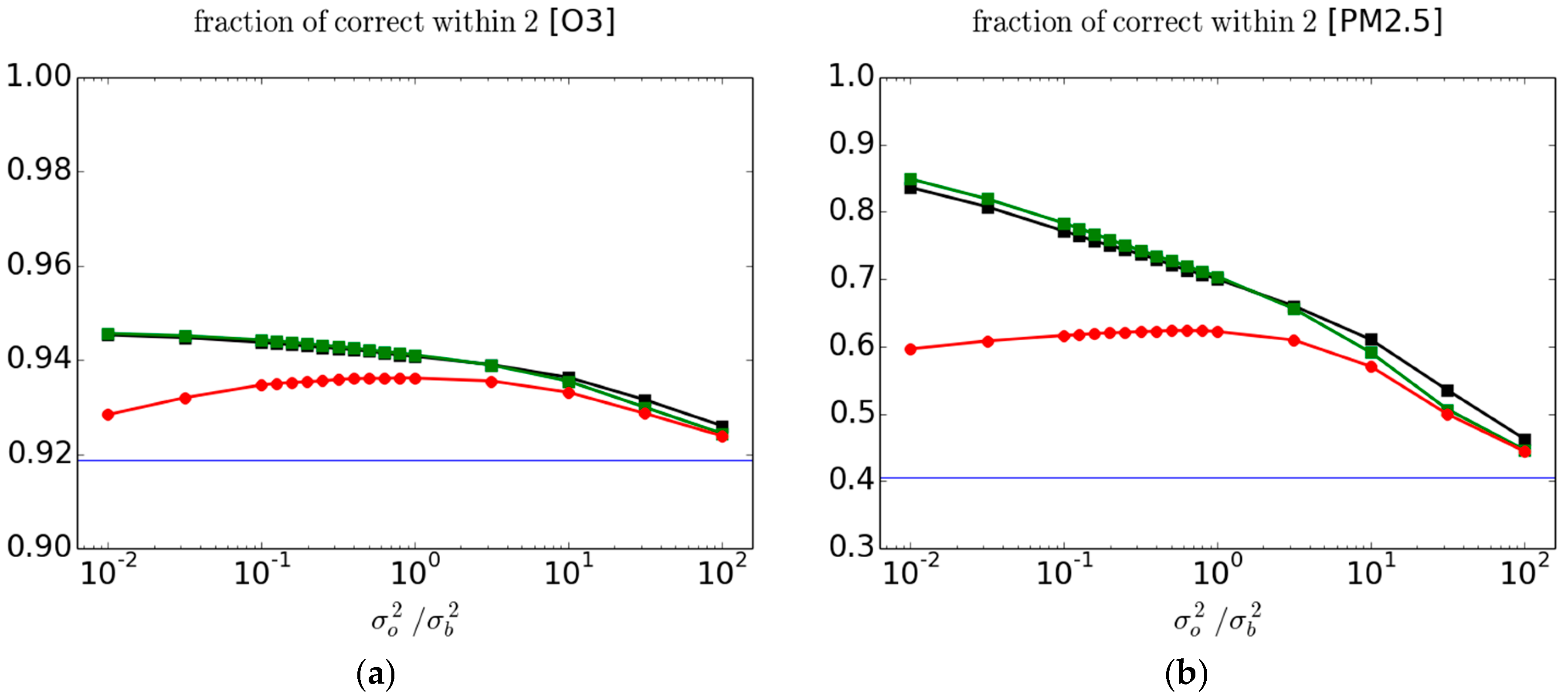
Another metric that we have considered is the FC2, Equation (5) [3]. The evaluation of this metric against passive and active observations is presented in Figure 4 for O3 (left panel) and PM2.5 (right panel). Note that the scale in the ordinate is quite different between the left and right panels. Although the results bear similarity with the correlation between O and A presented in Figure 3, the maximum with passive observations is reached at larger values than those obtained for or , which are identical. Individual fold results are presented in the supplementary materials Figure S3.
The interpretation of this metric is, however, not clear. Although the ratio is a dimensionless quantity the spread of is generally not independent of the variance of A or O and there are cases where it is. So to count the number of occurrence of between the dimensionless values 0.5 and 2 is confusing. As a simplified illustration, suppose that A is normally distributed as and similarly with . The ratio of these two random variables is then a Cauchy distribution whose probability density function (pdf) is . The mean, variance and higher moments of Cauchy probability distributions are not defined since the integral of the pdf is not bounded; only the mode is defined. Cauchy distributions also have a spread parameter, which in this case is equal to . If the variance of A and O are equal, then the number count between the dimensionless bounds 0.5 and 2 depends only on the shape of the probability distribution function, not on the variance. If the variance of A and O are different, then it also depends on the ratio of variances. Furthermore, in principle this metric also depends on the bias (which is not the case here for these analyses). It may be a difficult metric to interpret but if used as a quality control, the FC2 have the unique ability of rejecting too low as well as too high values of .
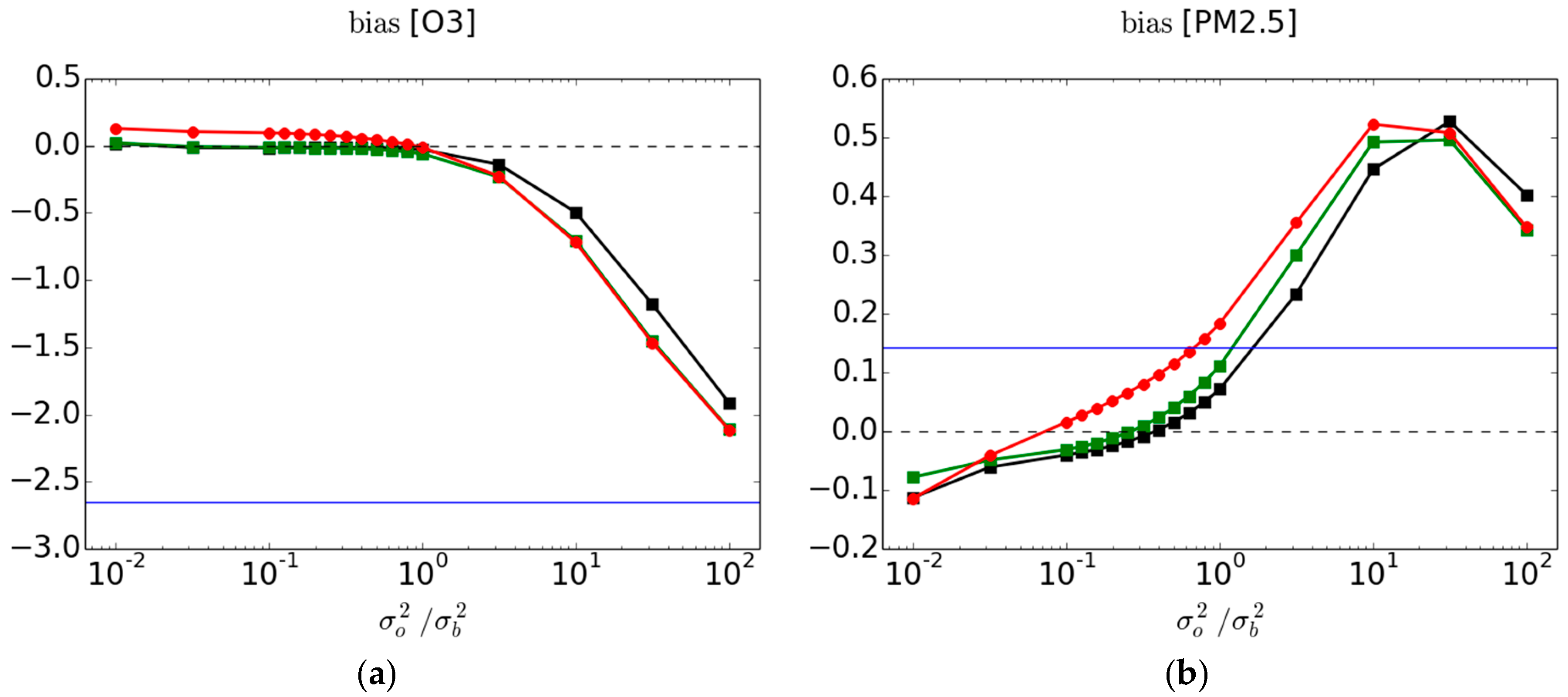
In Figure 5 we present the bias between observations and analyses, and where the verification is made against passive and active observations as done with the other metrics. Bias is not a dimensionless quantity; note that the range and scale presented for O3 and PM2.5 in Figure 5 are different. The blue curve is the mean and thus indicates that for O3 in average over all observation stations (for the time and dates considered) the model overpredicts, and that for PM2.5 the model underpredicts.
Contrary to all metric results seen so far, the 3-fold variability of the bias is substantial: it is of the order of ppbv (in average) for O3 at passive sites and of the order of (in average) for the PM2.5 at passive sites (results shown in the supplementary material Figure S4). The distinction between the red, black and green curves may not be statistically significant for both O3 and PM2.5. However, the difference between the analysis bias and model bias is large and statistically significant (see supplementary material). For O3, the model bias is eliminated at the passive observation sites (red curve) as long as the observation weight . The situation is not so clear for PM2.5. In fact, when the observation weight is small, we get the intruiging result that the bias of the analysis is larger bias than the model. How can that be when the observation weight is small (i.e., ); should the analysis not be close to the model values? This apparent contradiction reveals a more complex issue underlying the bias metric.
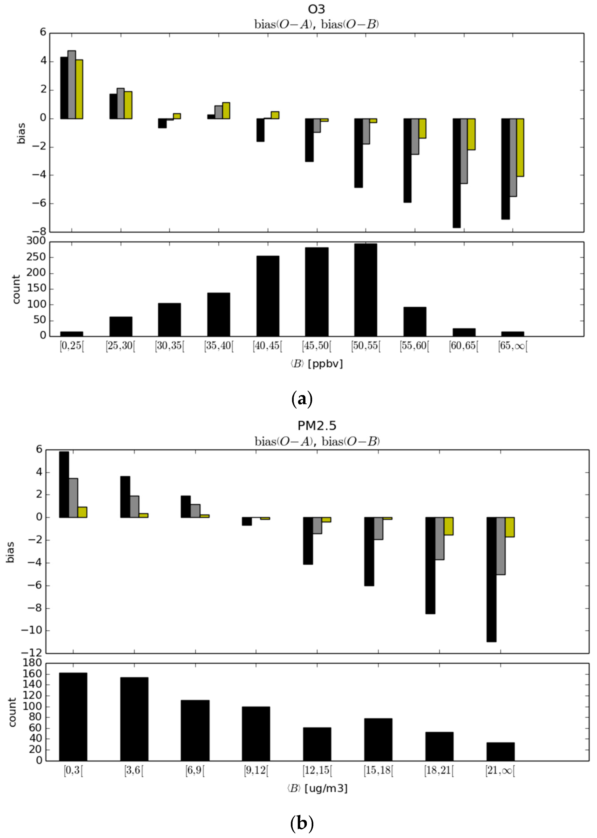
To explore the possible causes, we have calculated the bias per bin of model values, displayed in Figure 6. In order to have a decent sample size per bin, we collect all the and over time and observation sites, create bins of model values and calculate the statistic per bin (and not per station as before). The result shows that the model bias is nearly linearly dependent on the model values (black boxes in the bias panel). Both O3 and PM2.5 show an underprediction for low model values and an overprediction for large model values. The origin of this bias is not known but one would argue that it is not directly related to chemistry as such since both constituents, O3 and PM2.5, present the same feature. Possible explanations could be related to the model boundary layer, the emissions being too low for low polluted areas and too large for polluted areas, insufficient transport away from polluted areas to unpolluted areas, species destruction/scavenging could be too low in low polluted areas and too high in polluted areas. The lower panels of Figure 6a,b show the count of stations per model bin size. We observe that the majority of stations have O3 model values in the range of 40 to 55 ppbv, where the bias is negative. Over all the stations, this gives rise to a negative mean , and this is how we make the claim that the model overpredicts. However, for PM2.5 the situation is different: the majority of stations lie in the low model value range, and there are gradually less stations for increasingly larger model values. Although the have large negative values in the high model value bin while small model value bins have positives ’s, the effect over all stations is to yield a modestly positive mean and thus the model underestimates the PM2.5. The results of the analysis evaluated at the passive observation sites are presented with the yellow and grey histogram boxes. In yellow, near optimal analyses with optimal observation weight, as determined by the minimum of are used, and in grey non-optimal analyses with .
We observe that the effect of the optimal analysis is nearly insentive to model bin values, where near zero biases are obtained in most of the range except for very small and very large model values. The fact that we are not able to capture the full benefit of analysis on all model values may be an artefact of the assumption that we are using uniform observation and background error variances whereas the model values varies considerably. In grey, we used the non-optimal analyses with a small observation weight were we set . In the non-optimal case, the state-dependent bias is still present but appears to be nearly perfectly anti-symmetric, positive in the low model value bins and nearly the exact opposite in high model value bins. Since for O3 the majority of observations lie in the range 40 to 55 ppbv, for the optimal analyses at passive observation sites is nearly zero. However, for the non-optimal analysis with , the at passive sites is negative, i.e., the analysis is overpredicting, as shown in Figure 5.
For PM2.5, the weighted sum of the bins is such that over all stations the bias for an optimal analysis is nearly zero. In the case of the non-optimal analysis with , the weighted sum of the nearly anti-symmetric bias per bin gives more weight to the positive bias at smaller model values, so that overall there is a positive , as in Figure 5.
To circumvent the state-dependency of the biases it is useful to consider instead a fractional bias metric, such as the modified normalized mean bias, MNMB Equation (4). The MNMB metric is a dimensionless measure and as defined with a factor of 2, Equation (4), represents a % error. The MNMB metric is a relative measure with respect to the mean observed-analysis value and is thus less sensitive to spatially varying distribution of the concentrations, revealing instead the intrinsic difference between the fields. The MNMB for O3 and PM2.5 for passive and active observations are displayed in Figure 7 using the same color as in Figure 2. We note immediately that the MNMB analysis bias does not exceed the MNMB model bias as we observed for the bias metric of PM2.5 (Figure 5 right panel). The MNMB bias also varies smoothly as a function of (at variance with the bias metric for PM2.5—Figure 5).
Furthermore, examining the 3-fold variability of the cross-validation analysis MNMB at the passive sites and the variability of the MNMB at the active sites (see Figure S5 in supplementary materials), we infer that for PM2.5, where we can actually deduce that the difference between the cross-validation and the validation against active observations is statistically significant when . There is also another important point to make; although analyses are designed to reduce the error variance, it so happens that for a near optimal analysis the fractional bias MNMB is very small, around 1% for O3 and about 1–2% for PM2.5. We argue that it results from an optimal use of observations.
There is also some information to gain from the variance of observed-minus-analysis per bin size, as illustrated in Figure 8, using the same color histograms as in Figure 6. We note that for O3, the model error variance against observations increases gradually with larger model values. However, the fraction of analysis variance vs. model variance is roughly uniform across all bins. This can be explained by the fact that the observation and background error variances are uniform, and thus the reduction of variance across all bins is uniform as well. However, the situation is different for PM2.5. We note a relatively poor performance of the model at low model values, with standard deviation of 7 μg/m3. For slightly larger model values (3–6 μg/m3), the error variance is smaller to 5.5 μg/m3 and then increases almost linearly with model values. The fraction of analysis variance vs. model variance decreases steadily with larger model values. These results thus indicate that the assumption that observation and background error variances are uniform and independent of the model value may have to be revisited.
4. Conclusions
We have developed an approach by which analyses can be evaluated and optimized without using a model forecast but rather by partitioning the original observation data set into a training set, to create the analysis, and an independent (or passive) set, used to evaluate the analysis. This kind of evaluation by partitioning is called cross-validation.
The need for such a technique came about from our desire to evaluate our operational surface air quality analyses that are created off-line with no assimilation cycling. Evaluating a surface air quality analysis based on its chemical forecast does in fact require additional information or assumptions, such as vertical correlation, aerosol speciation and bin distribution (while surface measurement is primarily about mass) or unobserved chemical variables correlations, and so on. So that the quality of the chemical forecast is not solely dependent on the quality of the analysis and, if there are compensating errors, can actually be a misleading assessment of the quality of the analysis.
We have applied this cross-validation procedure to the operational analyses of surface O3 and PM2.5 over North America for a period of 60 days and present an evaluation using different metrics; bias, modified normalized mean bias, variance of observation-minus-analysis residuals, correlation between observation and analysis, and fraction of correction within a factor of 2.
Our results show that, in terms of variance and correlation, the verification of analyses against active observations always yield an overestimation of the accuracy of the analysis. This overestimation also increases as the observation weight increases. On the other hand for biases, the distinction between the verification against active observations and passive observations is unclear and drowned in the sample variability. However, using a fractional bias metric, in particular the MNMB, shows that the verification against passive observations can be close to one percent for an optimal analysis while the verification against active observations is much larger.
Results also show the importance of having an optimal analysis for verification. The variance of the analysis with respect to independent observations is minimum and the correlation between the analysis and independent observations is maximum for an optimal analysis. By being a compromise between an overfit to the active observations (which produce noisy analysis field) and an underfit, the optimal analysis offers the best use of observations throughout. At optimality, the analysis fractional bias (MNMB) at the passive observation sites has only one or two percent error whereas the fractional bias of the model is 6.5% for O3 and 21% for PM2.5. The correlation between the analysis and independent observations is also significantly improved with an optimal analysis: the correlation between the model and independent observations is 0.55 for O3 and increases to 0.74 with the analysis, while for PM2.5 the correlation between the model and independent observations is only 0.3 (which is basically no skill) but rises to 0.54 for the analysis.
We also argue that the fraction of correct within a factor of 2, is a metric whose interpretation is unclear as it mixes information about bias, variance and probability distribution in a non-uniform way and does not seem to add anything new to other metrics. The bias is also very sensitive to sample variability and can lead to wrong conclusions. For example, we have seen that the mean analysis bias can be larger than the mean model bias, whether verifying against active or passive observations. However, since an analysis is always closer to the truth than its prior (i.e., the model), it results in an apparent contradiction. This implies that the bias metric cannot be used to faithfully compare model states accurately. Such wrongful conclusions do not arise, however, with the MNMB. We thus recommend avoiding using bias as a measure of truthfulness, and use instead a fractional bias measure such as the MNMB.
We also found that errors in the GEM-MACH model grow almost linearly with the model value. This is particularly evident for the bias where the model underestimates at small model values and overestimates at large model values. Furthermore, this occurs in equal ways for O3 and PM2.5, thus indicating that the source of this bias is not related to chemistry. The fact that, over the entire domain, the model overestimates O3, and underestimates PM2.5 is simply a result of the concentrations. We have not conducted a systematic study of model error for other times of the day and other periods of the year, but it would be very interesting to look at this, to see whether or not changes of biases are due primarily to changes in the distribution of values rather than a fundamental change in the bias per model value bin.
Finally, we have also examined the variance against independent observations per model value bin, and concluded that the error variance is not quite uniform with model values but increases slowly with model values for O3 and in a more pronounced way for PM2.5.
In part two, we will focus on the estimation of the analysis error variance and develop a mathematical formalism that permits the comparison of different diagnostics of variance under different assumptions, optimizes the analysis parameters and gains confidence on the estimate of analysis error as we obtain coherent estimated values across different diagnostics.
Supplementary Materials
The following are available online at https://www.mdpi.com/2073-4433/9/3/86/s1, Figure S1: Verification of variance for O3 and PM2.5 for the individual sets. Figure S2: Same as Figure S1 but for the correlation between observations and analysis. Figure S3: Same as Figure S1 but for the fraction of correct within a factor of 2. Figure S4: Same as Figure S1 but for bias. Figure S5: Same as Figure S1 but for modified normalized mean bias.
Acknowledgments
We are grateful to the US/EPA for the use of the AIRNow database for surface pollutants and to all provincial governments and territories of Canada for kindly transmitting their data to the Canadian Meteorological Centre to produce the surface analysis of atmospheric pollutants. We are also thankful for the proof read by Kerill Semeniuk, and for three anonymous reviewers for their comments and help in improving the manuscript.
Author Contributions
This research was conducted as a joint effort by both authors. R.M. contributed to the theoretical development and wrote the paper, and M.D.-J. conducted all experiments design and execution, proof reading and introduced a new diagnostic of optimal analysis error that was furher extended to passive observations space.
Conflicts of Interest
The authors declare no conflict of interest. The founding sponsors, which is the government of Canada, had no role in the design of the study; in the collection, analyses, or interpretation of data; in the writing of the manuscript, and in the decision to publish the results.
References
- Ménard, R.; Robichaud, A. The chemistry-forecast system at the Meteorological Service of Canada. In Proceedings of the ECMWF Seminar Proceedings on Global Earth-System Monitoring, Reading, UK, 5–9 September 2005; pp. 297–308. [Google Scholar]
- Robichaud, A.; Ménard, R. Multi-year objective analysis of warm season ground-level ozone and PM2.5 over North-America using real-time observations and Canadian operational air quality models. Atmos. Chem. Phys. 2014, 14, 1769–1800. [Google Scholar] [CrossRef]
- Robichaud, A.; Ménard, R.; Zaïtseva, Y.; Anselmo, D. Multi-pollutant surface objective analyses and mapping of air quality health index over North America. Air Qual. Atmos. Health 2016, 9, 743–759. [Google Scholar] [CrossRef] [PubMed]
- Moran, M.D.; Ménard, S.; Pavlovic, R.; Anselmo, D.; Antonopoulus, S.; Robichaud, A.; Gravel, S.; Makar, P.A.; Gong, W.; Stroud, C.; et al. Recent Advances in Canada’s National Operational Air Quality Forecasting System, 32nd ed.; Springer: Dordrecht, The Netherlands, 2014. [Google Scholar]
- Pudykiewicz, J.A.; Kallaur, A.; Smolarkiewcz, P.K. Semi-lagrangian modelling of tropospheric ozone. Tellus B 1997, 49, 231–248. [Google Scholar] [CrossRef]
- Cressie, N.; Wikle, C.K. Statistics for Spatio-Temporal Data; Wiley: Hoboken, NJ, USA, 2011. [Google Scholar]
- Schneider, P.; Castell, N.; Vogt, M.; Dauge, F.R.; Lahoz, W.A.; Bartonova, A. Mapping urban air quality in near real-time using observations from low-cost sensors and model information. Environ. Int. 2017, 106, 234–247. [Google Scholar] [CrossRef] [PubMed]
- Lindström, J.; Szpiro, A.A.; Oron, P.D.; Richards, M.; Larson, T.V.; Sheppard, L. A flexible spatio-temporal model for air pollution and spatio-temporal covariates. Environ. Ecol. Stat. 2014, 21, 411–433. [Google Scholar] [CrossRef] [PubMed]
- Carmichael, G.R.; Sandu, A.; Chai, T.; Daescu, D.N.; Constantinescu, E.M.; Tang, Y. Predicting air quality: Improvements through advanced methods to integrate models and measurements. J. Comput. Phys. 2008, 227, 3540–3571. [Google Scholar] [CrossRef]
- Dabberdt, W.F.; Carroll, M.A.; Baumgardner, D.; Carmichael, G.; Cohen, R.; Dye, T.; Ellis, J.; Grell, G.; Grimmond, S.; Hanna, S.; et al. Meteorological research needs for improved air quality forecasting: Report of the 11th prospectus development team of the US weather research program. Bull. Am. Meteorol. Soc. 2004, 85, 563–586. [Google Scholar] [CrossRef]
- Sportisse, B. A review of current issues in air pollution modeling and simulation. Comput. Geosci. 2007, 11, 159–181. [Google Scholar] [CrossRef]
- Elbern, H.; Strunk, A.; Nieradzik, L. Inverse modelling and combined state-source estimation for chemical weather. In Data Assimilation; Lahoz, W., Khattatov, B., Ménard, R., Eds.; Springer: Berlin/Heidelberg, Germany, 2010; pp. 491–513. [Google Scholar]
- Bocquet, M.; Elbern, H.; Eskes, H.; Hirtl, M.; Žabkar, R.; Carmicheal, G.R.; Flemming, J.; Inness, A.; Pagaoski, M.; Pérez Camaño, J.L.; et al. Data assimilation in atmospheric chemistry models; current status and future prospects for coupled chemistry meteorology models. Atmos. Chem. Phys. 2015, 15, 5325–5358. [Google Scholar] [CrossRef] [Green Version]
- Chai, T.; Carmichael, G.R.; Sandu, A.; Tang, Y.H.; Daescu, D.N. Chemical data assimilation of transport and chemical evolution over the pacific (TRACE-P) aircraft measurements. J. Geophys. Res. 2006, 111, D02301. [Google Scholar] [CrossRef]
- Sandu, A.; Chai, T. Chemical data assimilation—An overview. Atmosphere 2011, 2, 426–463. [Google Scholar] [CrossRef]
- Marseille, G.J.; Barkmeijer, J.; De Haan, S.; Verkle, W. Assessment and tuning of data assimilation systems using passive observations. Q. J. R. Meteorol. Soc. 2016, 142, 3001–3014. [Google Scholar] [CrossRef]
- Ménard, R.; Deshaies-Jacques, M.; Gasset, N. A comparison of correlation-length estimation methods for the objective analysis of surface pollutants at Environment and Climate Change Canada. J. Air Waste Manag. Assoc. 2016, 66, 874–895. [Google Scholar] [CrossRef] [PubMed]
- Cohn, S.E.; Da Silva, A.; Guo, J.; Sienkiewicz, M.; Lamich, D. Assessing the effects of data selection with the DAO physical-space statistical analysis system. Mon. Weather Rev. 1998, 126, 2913–2926. [Google Scholar] [CrossRef]
- Houtekamer, P.L.; Mitchell, H.L. A sequential ensemble Kalman filter for atmospheric data assimilation. Mon. Weather Rev. 2001, 129, 123–137. [Google Scholar] [CrossRef]
- Efron, B.; Tibshirani, R.J. An Introduction to Boostrap; Chapman & Hall: New York, NY, USA, 1993. [Google Scholar]
- Seigneur, C.; Pun, B.; Pai, P.; Louis, J.F.; Solomon, P.; Emery, C.; Morris, R.; Zahniser, M.; Worsnop, D.; Koutrakis, P.; et al. Guidance for the performance evaluation of three-dimensional air quality modeling systems for particulate matter and visibility. J. Air Waste Manag. Assoc. 2000, 50, 588–599. [Google Scholar] [CrossRef] [PubMed]
- Chang, J.C.; Hanna, S.R. Air quality model performance evaluation. Meteorol. Atmos. Phys. 2004, 87, 167–196. [Google Scholar] [CrossRef]
- Savage, N.H.; Agnew, P.; Davis, L.S.; Ordóñez, C.; Thorpe, R.; Johnson, C.E.; O’Connor, F.M.; Dalvi, M. Air quality modelling using the Met Office Unified Model (AQUM OS24-26): Model description and initial evaluation. Geosci. Model Dev. 2013, 6, 353–372. [Google Scholar] [CrossRef]
- Katragkou, E.; Zanis, P.; Tsikerdekis, A.; Kapsomenakis, J.; Melas, D.; Eskes, H.; Flemming, J.; Huijnen, V.; Inness, A.; Schultz, M.G.; et al. Evaluation of near surface ozone over Europe from the MACC reanalysis. Geosci. Model Dev. 2015, 8, 2299–2314. [Google Scholar] [CrossRef]
- Ménard, R. Error covariance estimation methods based on analysis residuals: Theoretical foundation and convergence properties derived from simplified observation networks. Q. J. R. Meteorol. Soc. 2016, 142, 257–273. [Google Scholar] [CrossRef]
- Desroziers, G.; Berre, L.; Chapnik, B.; Poli, P. Diagnosis of observation, background, and analysis-error statistics in observation space. Q. J. R. Meteorol. Soc. 2005, 131, 3385–3396. [Google Scholar] [CrossRef]
- Daley, R. Atmospheric Data Analysis; Cambridge University Press: New York, NY, USA, 1991; p. 457. [Google Scholar]
- Ménard, R.; Deshaies-Jacques, M. Evaluation of analysis by cross-validation, Part II: Diagnostic and optimization of analysis error covariance. Atmosphere 2018, 9, 70. [Google Scholar] [CrossRef]
Figure 1.
Spatial distribution of the three subsets of PM2.5 observations used for cross-validation. The selection algorithm is based on regular picking of station by ID number.
Figure 1.
Spatial distribution of the three subsets of PM2.5 observations used for cross-validation. The selection algorithm is based on regular picking of station by ID number.

Figure 2.
Variance of observation-minus-analysis residuals of O3 and PM2.5 for both active and cross-validation passive observations as a function of . (a) is for O3 with ordinates in ppbv2 units, and (b) is for PM2.5 with ordinates in . Red curve results from the evaluation at the passive observation sites (average of the 3-fold subsets). Black curve results from evaluation at the active observation sites with analyses using all observations. Green curve results from the evaluation at the active observation sites in the cross-validation experiment (i.e., using 2/3 of the observations; average of the three subsets). Blue curve is the variance of observation-minus-model.
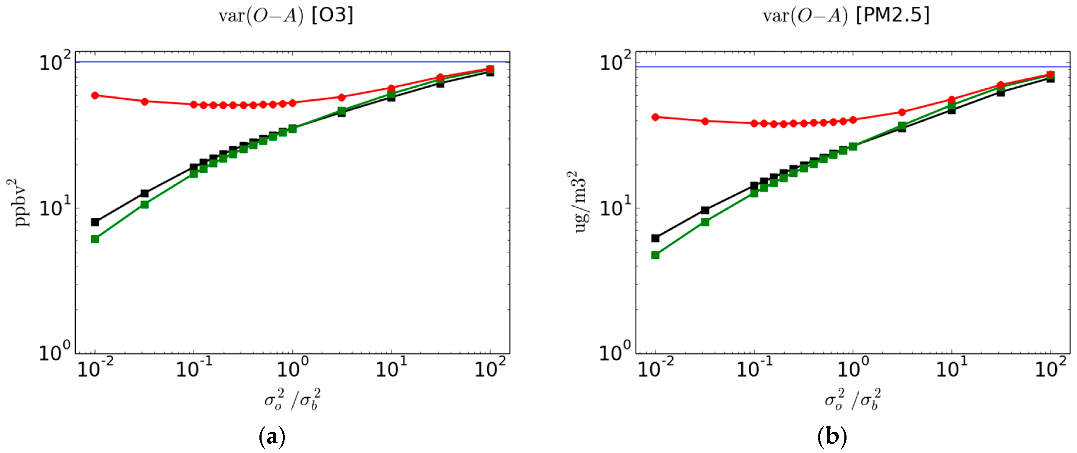
Figure 3.
Correlation between observations and analysis for (a) O3 and (b) PM2.5 for both active and cross-validation passive observations as a function of . The red, black and green curves are as in Figure 2.
Figure 3.
Correlation between observations and analysis for (a) O3 and (b) PM2.5 for both active and cross-validation passive observations as a function of . The red, black and green curves are as in Figure 2.

Figure 4.
FC2 for (a) O3 and (b) PM2.5 for both active and cross-validation passive observations as a function of . The red, black and green curves are as in Figure 2.
Figure 4.
FC2 for (a) O3 and (b) PM2.5 for both active and cross-validation passive observations as a function of . The red, black and green curves are as in Figure 2.

Figure 5.
Bias between observation and analysis for (a) O3 and (b) PM2.5 for both active and cross-validation passive observations as a function of . The red, black and green curves are as in Figure 2.
Figure 5.
Bias between observation and analysis for (a) O3 and (b) PM2.5 for both active and cross-validation passive observations as a function of . The red, black and green curves are as in Figure 2.

Figure 6.
Biases per bin of model values. Figure (a), presents the statistics for O3 and in (b), for PM2.5. In the upper portion, (a,b) are the residual statistics per bin; in black, the , in grey, the at passive observation sites (mean of the 3-fold subsets) for a non-optimal analysis with , and in yellow, the at passive observation sites (mean of the 3-fold subsets) using the optimal observation weight. In the lower portion, (a,b) are the station number count per model values.

Figure 7.
Modified normalized mean bias (MNMB) between observation and analysis for (a) O3 and (b) PM2.5 for both active and cross-validation passive observations as a function of . The red, black and green curves are as in Figure 2.
Figure 7.
Modified normalized mean bias (MNMB) between observation and analysis for (a) O3 and (b) PM2.5 for both active and cross-validation passive observations as a function of . The red, black and green curves are as in Figure 2.
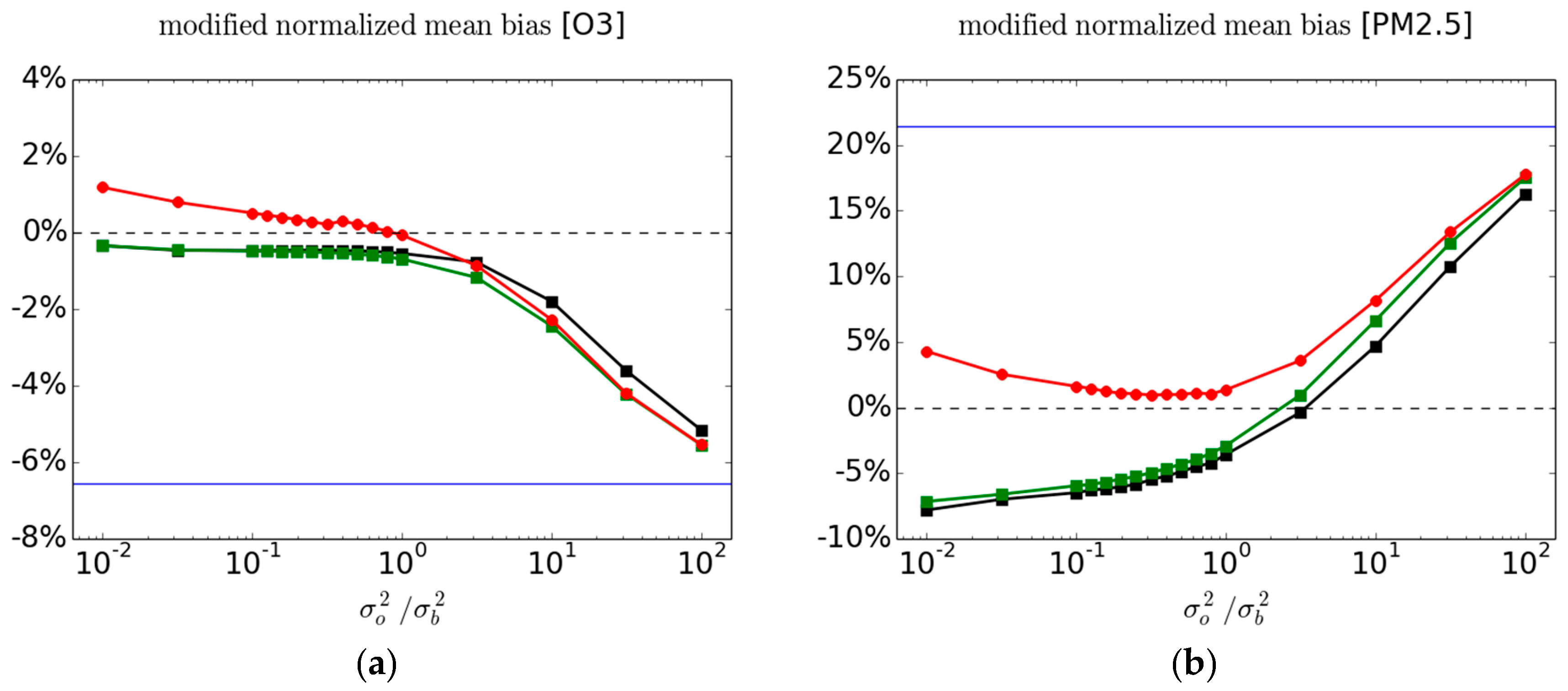
Figure 8.
Figure 8. Same as Figure 6 except that we display the variance of analysis-minus-passive observations per bin of model values.
Figure 8.
Figure 8. Same as Figure 6 except that we display the variance of analysis-minus-passive observations per bin of model values.

© 2018 by the authors. Licensee MDPI, Basel, Switzerland. This article is an open access article distributed under the terms and conditions of the Creative Commons Attribution (CC BY) license (http://creativecommons.org/licenses/by/4.0/).
Share and Cite
MDPI and ACS Style
Ménard, R.; Deshaies-Jacques, M. Evaluation of Analysis by Cross-Validation. Part I: Using Verification Metrics. Atmosphere 2018, 9, 86. https://doi.org/10.3390/atmos9030086
AMA Style
Ménard R, Deshaies-Jacques M. Evaluation of Analysis by Cross-Validation. Part I: Using Verification Metrics. Atmosphere. 2018; 9(3):86. https://doi.org/10.3390/atmos9030086
Chicago/Turabian StyleMénard, Richard, and Martin Deshaies-Jacques. 2018. "Evaluation of Analysis by Cross-Validation. Part I: Using Verification Metrics" Atmosphere 9, no. 3: 86. https://doi.org/10.3390/atmos9030086
Note that from the first issue of 2016, this journal uses article numbers instead of page numbers. See further details here.