Precipitation Extended Linear Scaling Method for Correcting GCM Precipitation and Its Evaluation and Implication in the Transboundary Jhelum River Basin

Abstract

In this study, a linear scaling method, precipitation extended linear scaling (PELS), is proposed to correct precipitation simulated by GCMs. In this method, monthly scaling factors were extended to daily scaling factors (DSFs) to improve the daily variation in precipitation. In addition, DSFs were also checked for outliers and smoothed with a smoothing filter to reduce the effect of noisy DSFs before correcting the GCM’s precipitation. This method was evaluated using the observed precipitation of 21 climate stations and five GCMs in the Jhelum River basin, Pakistan and India, for the period of 1986–2000 and also compared with the original linear scaling (OLS) method. The evaluation results showed substantial improvement in the corrected GCM precipitation, especially in case of mean and standard deviation values. Although PELS and OLS showed comparable results, the overall performance of PELS was better than OLS. After Evaluation, PELS was applied to the future precipitation from five GCMs for the period of 2041–2070 under RCP8.5 and RCP2.6 in the Jhelum basin, and the future changes in precipitation were calculated with respect to 1971–2000. According to average all GCMs, annual precipitation was projected to decrease by 4% and 6% in the basin under RCP8.5 and RCP2.6, respectively. Although two seasons, spring and fall, showed some increasing precipitation, the monsoon season showed severe decrease in precipitation, with 22% (RCP8.5) and 29% (RCP2.6), and even more reduction in July and August, up to 34% (RCP8.5) and 36% (RCP2.6). This means if the climate of the world follows the RCP8.5 and RCP2.6, then there will be a severe reduction in precipitation in the Jhelum basin during peak months. It was also observed that decline in precipitation was higher under RCP2.6 than RCP8.5.

1. Introduction

Recently, Global Climate Models (GCMs) are the most advanced numerical tools to understand the global climate system encompassing the atmosphere, oceans, and sea-ice [1,2] in order to project the global climate; and to investigate the potential changes in climate. However, these models simulate outputs on a large grid size, ranging from 100 to 300 km horizontally, [3] which restrict their direct applications in the studies related environmental and hydrological assessment on local scale or basin scales [4]. To use these outputs at local or regional level, downscaling techniques are needed to make a bridge between GCM’s outputs and local/regional climatic variables (e.g., temperature, wind speed, and precipitation) [5]. There are two major categories of downscaling: dynamical and statistical. In dynamical downscaling, a high-resolution climate model, Regional Climate Model (RCM), simulates outputs at a fine resolution of about 5 to 50 km, using the coarse outputs of a GCM [6,7,8]. However, there are the chances of systematic errors in RCM’s outputs that inhabit to GCMs. The capability of RCMs mostly depends on GCM’s driving forces. In addition, the computational increases required to run an experiment as the resolution and domain size increases confines the study areas and the number of experiments to generate climate scenarios [1,9].

Statistical downscaling (SD) methods create statistical relationships between GCM’s outputs and observations. These are much faster, simpler, and computationally inexpensive relative to dynamic downscaling (DD) techniques, and therefore, the wider community of scientists has rapidly been adopting these methods in climate and hydrology related studies [4,5,8]. Recently, many statistical models such as Statistical Downscaling Model (SDSM) [10], Automated Statistical Downscaling model (ASD) [11], and Lars Weather Generator (LARS-WG) [12] have been developed to downscale climate variables. However, these methods require historical observations over a long period (e.g., 30 years) to establish suitable linkages with GCM outputs, and this relationship is assumed to be temporally stationary [9].

Linear scaling techniques are much simpler and faster methods than both SD and DD methods for using the outputs of GCMs at regional scale. In these methods, biases are removed from GCM outputs or RCM outputs. The fundamental difference in SD and bias correction method is that in SD statistical, empirical relationships are created between local-scale variable (e.g., temperature or precipitation) and large-scale variables (e.g., specific humidity, sea level pressure, and temperature of GCMs), and then data is simulated for the future period on the basis of these relationships along with the same projected large scale variables. In contrast, bias correction method simply corrects the biases in simulated GCM outputs (e.g., temperature and precipitation) [13,14]. Several scaling methods have been developed in which some methods are quite simple and easy to apply as with linear scaling methods, and some are sophisticated, such as probability mapping and distribution mapping. Basically, these were used to correct the outputs of GCMs and now are also applied for RCM outputs [15]. The following six methods have been stated in the literature: (1) local intensity scaling method for precipitation; (2) linear scaling methods for precipitation and temperature; (3) power transformation for precipitation; (4) distribution mapping for temperature and precipitation; (5) delta change for both temperature and precipitation; and (6) temperature-variance scaling. Detailed discussion about these methods is reported in these studies [15,16].

The following are the two main steps in all linear scaling methods that are used to correct GCM outputs except the delta change method: the first step is to calculate scaling factors (SFs) between observations and GCM’s outputs, and the second step is to adjust these SFs with the projected outputs of GCMs. On the other hand, in delta change method, change factors (CFs) are first obtained from the simulated data of GCMs for the present period, e.g., 1961–1990, and for the future period, e.g., 2041–2070, and secondly, the CFs are adjusted with the observations to generate perturbed future time series (e.g., 2041–2070). The central step in all scaling methods is the calculation of SFs. These SFs have been calculated by different techniques reported in the literature. In some studies such as [17,18] during the 1990s, these were calculated by subtracting a long-period (e.g., 30 year) observed mean from a long-period simulated mean in the case of temperature and by dividing in the case of precipitation. This means that the only one value as a SF was used to adjust the daily or monthly GCM future temperature or precipitation to obtain out the corrected future data.

Recently, in the case of linear scaling methods, SFs are obtained from long-term (e.g., 30 year) monthly mean values of the simulated GCM data and observed data as in [15,16,19,20]. In this way, twelve mean monthly SFs are estimated, and then these are adjusted with the future simulated daily data of GCMs to reduce the biases. So, all days of a month are adjusted with one scaling factor calculated for that specific month. For example, to reduce biases from the future daily temperature of September, only one mean monthly SF of September is used for all the days of this month for the whole period. This linear scaling is good to measure mean changes in climate variables such as temperature for the future period. However, it confines its application in extreme data analyses.

There is a possibility that each month can have different SFs for different days. For example, each month (e.g., September) may have different SFs for the first day or week than the last day or week of that month. There are also chances that the performance (efficiency) of simulating data of a GCM might be different for different days of each month. For example, a GCM may simulate well in the first week than the last days. In addition, the simulation capability of different GCMs can be different for different days in each month. To overcome these problems, recently, Mahmood and Jia [21] have developed a method, extended linear scaling (ELS) method for temperature, by extending a linear scaling method to correct the temperature of GCMs or RCMs.

In the present study, we proposed a linear scaling technique, precipitation extended linear scaling (PELS), to correct the simulated future precipitation of GCMs. The procedure of proposed method is somehow similar to the extended linear scaling method for temperature by Mahmood and Jia [21] in terms of steps involved. However, for precipitation, we used different equations to calculate the daily scaling factors (DSFs), which were not the same as temperature. In addition, the DSFs calculated for precipitation were also checked for outliers before using them to correct precipitation, because during the calculation of DSFs, it was observed that some SFs were extraordinarily higher than other values, which might be outliers. This step was also not incorporated in extended linear scaling method for temperature by Mahmood and Jia [21]. This method can capture better variation (in case of magnitude) of observed data than the original scaling method because in this method, 30 different SFs are calculated for each month instead of only one SF as in the original scaling method. For example, if we correct precipitation with PELS method and used them for streamflow simulation in some snow- and glacier-dominated basins, this can provide better results as this method gives better daily variation than the original scaling method.

The proposed method was evaluated with the precipitation data of 5 GCMs, simulated for historical period, in the transboundary Jhelum River basin and then applied to correct the GCM precipitation simulated under RCP8.5 and RCP2.6. Before evaluation of PELS method, these GCM precipitations were compared with the historical observations to check the capability of this model to simulate precipitation, without any correction. In the end, the future changes in precipitation were estimated relative to the baseline period.

2. Study Area and Data Description

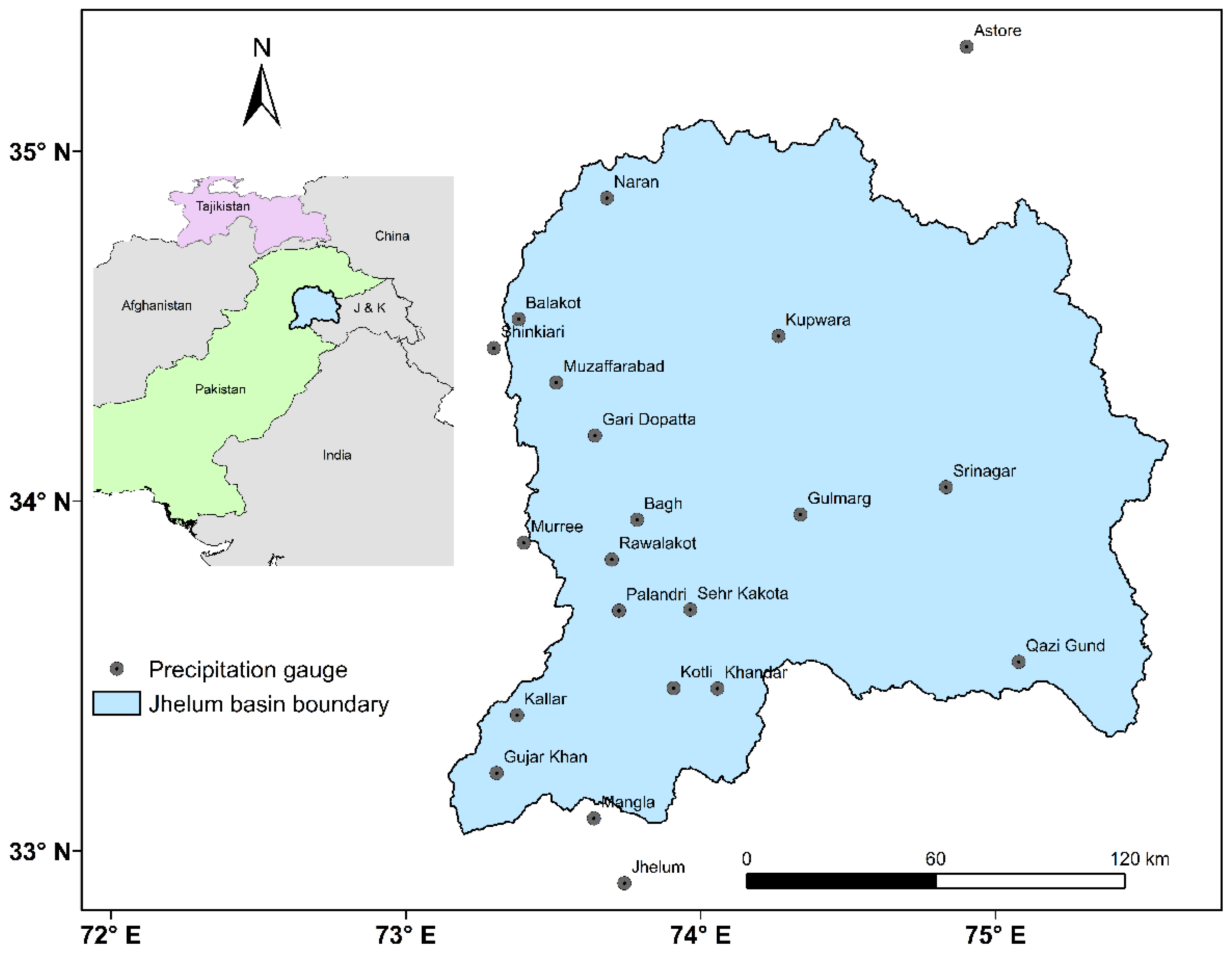
2.1. Study Area

The Jhelum River basin, located in the north of Pakistan and India, extends from 33° N to 35° N and 73° E to 75.62° E, as shown in Figure 1. The Jhelum basin with a drainage area of 33,342 km² ranges between an elevation of 235 m and 6285 m above sea level. The Jhelum River is of great importance to Pakistan because the Mangla Reservoir depends entirely on the streamflow of this river. This river contributes a mean annual discharge of 829 m³/s (989 mm/year) to Mangla Reservoir, the second largest reservoir in Pakistan. The reservoir’s primary objective is to store water for irrigation, and the secondary purpose is to produce hydropower. The basin receives an average annual precipitation of 1200 mm. However, most of the precipitation occurs in the monsoon season (July and August). An average annual temperature of 13.72 °C occurs over the basin, with Jhelum as the hottest climate station (23.53 °C) and Naran as the coldest climate station (6.14 °C). January, with an average temperature of 2.9 °C, and July, with an average temperature of 23 °C, are the coldest and hottest months, respectively, in the Jhelum basin [2,22].

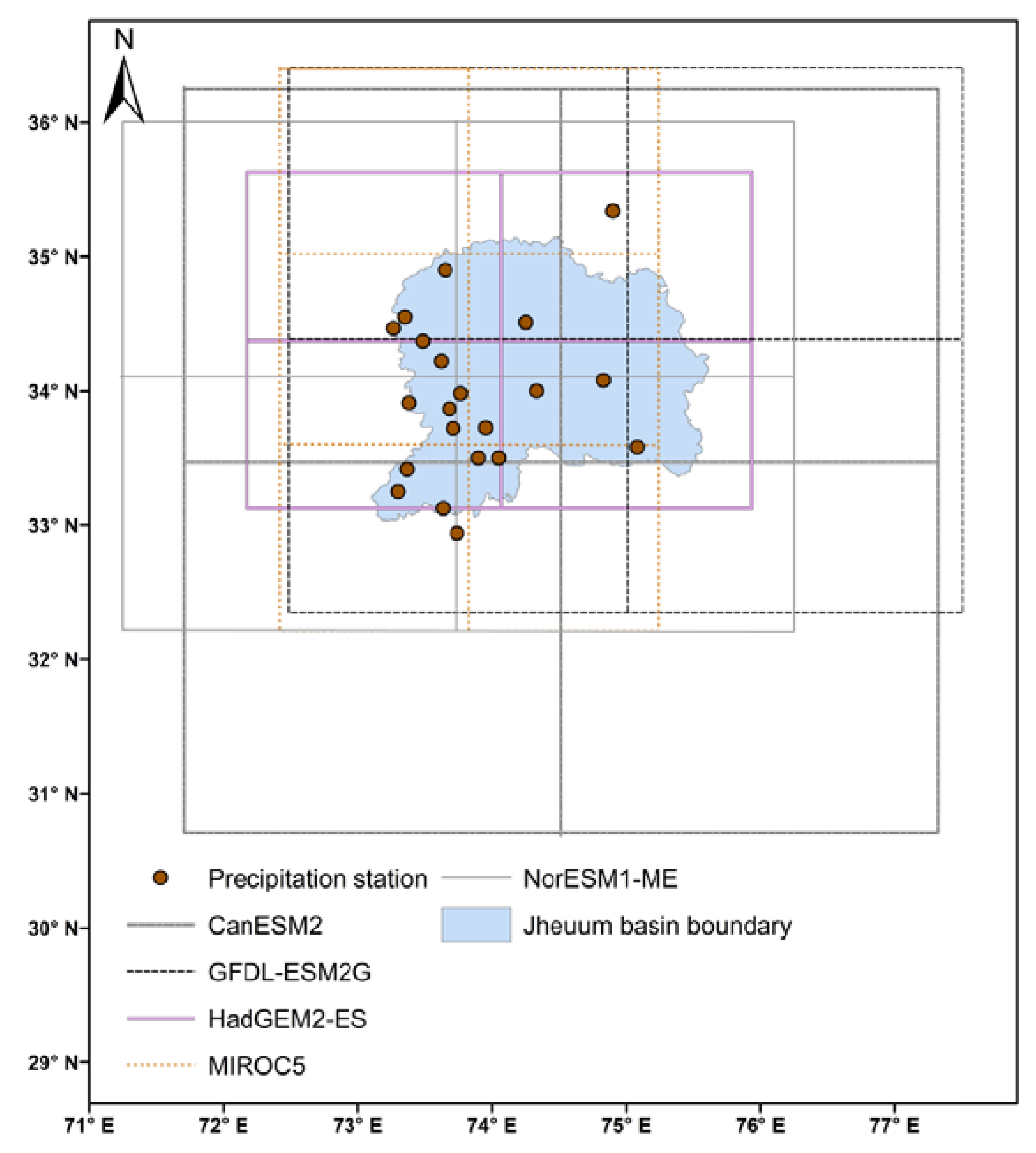
2.2. Data Description

Historical daily precipitation observations were collected from Pakistan Meteorological Department, the Water and Power Development Authority of Pakistan, and India Meteorological Department for 21 meteorological stations for the period 1971–2000. The basic information and location of these stations are shown in Figure 1 and described in

Table 1. Basic information about meteorological stations located in the Jhelum River basin.

Serial Number	Station	Latitude (°)	Longitude (°)	Elevation (m AMSL)	Annual Precipitation (mm)
1	Astore	35.34	74.90	2168	496
2	Bagh	33.98	73.77	1067	1496
3	Balakot	34.55	73.35	995	1529
4	Gari Dopatta	34.22	73.62	814	1483
5	Gujar Khan	33.25	73.30	457	881
6	Gulmarg	34.00	74.33	2705	1702
7	Jhelum	32.94	73.74	287	858
8	Kallar	33.42	73.37	518	988
9	Khandar	33.50	74.05	1067	1101
10	Kotli	33.50	73.90	614	1289
11	Kupwara	34.51	74.25	1609	1283
12	Mangla	33.12	73.63	305	863
13	Murree	33.91	73.38	2213	1805
14	Muzaffarabad	34.37	73.48	702	1508
15	Naran	34.90	73.65	2362	1640
16	Palandri	33.72	73.71	1402	1411
17	Qazi Gund	33.58	75.08	1690	1379
18	Rawalakot	33.87	73.68	1676	1407
19	Sehr Kakota	33.73	73.95	914	1471
20	Shinkiari	34.47	73.27	991	1312
21	Srinagar	34.08	74.83	1587	771

. India Meteorological Department provided precipitation data of Srinagar, Kupwara, Qazigund, and Gulmarg, and the rest of the data was obtained from Pakistan Meteorological Department.

Daily historical and future precipitation was obtained from CMIP5 project for 5 global climate models i.e., GFDL-ESM2G, HadGEM2-ES, NorESM1-ME, CanESM2, and MIROC5 [23]. The GCMs were chosen on basis of their good performance in the evaluation studies by [24,25] over South Asia. Hereafter, GFDL will be used for GFDL-ESM2G, NorESM1 for NorESM1-ME, and HadGEM2 for HadGEM2-ES. The simulated precipitation for the historical experiment and RCPs (i.e., RCP8.5 and RCP2.6) was obtained for 1971–2000 and 2041–2070, respectively. Some basic information of each model is provided in

Table 2. Description of five global climate models (GCMs) used in the present study.

Centre	Country	Model	Resolution Grid (Latitude × Longitude)
Geophysical Fluid Dynamics Laboratory (GFDL)	USA	GFDL-ESM2G	90 × 144
Norwegian Climate Centre (NCC)	Norway	NorESM1-ME	96 × 144
Met Office Hadley Centre (MOHC)	UK	HadGEM2-ES	145 × 192
Atmosphere and Ocean Research Institute (AORI)	Japan	MIROC5	128 × 256
Canadian Centre for Climate Modelling and Analysis (CCCMA)	Canada	CanESM2	64 × 128

, and their grids covering the study area are shown in Figure 2.

3. Methodology

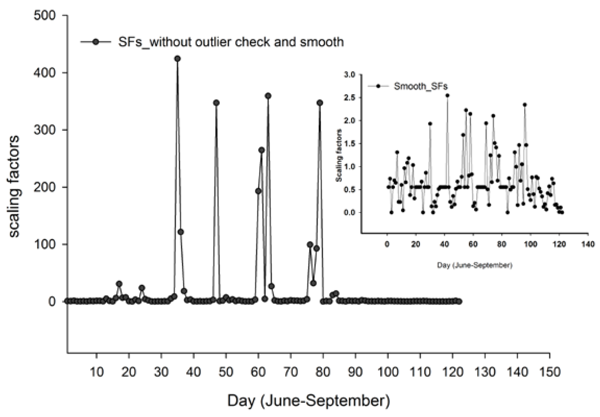
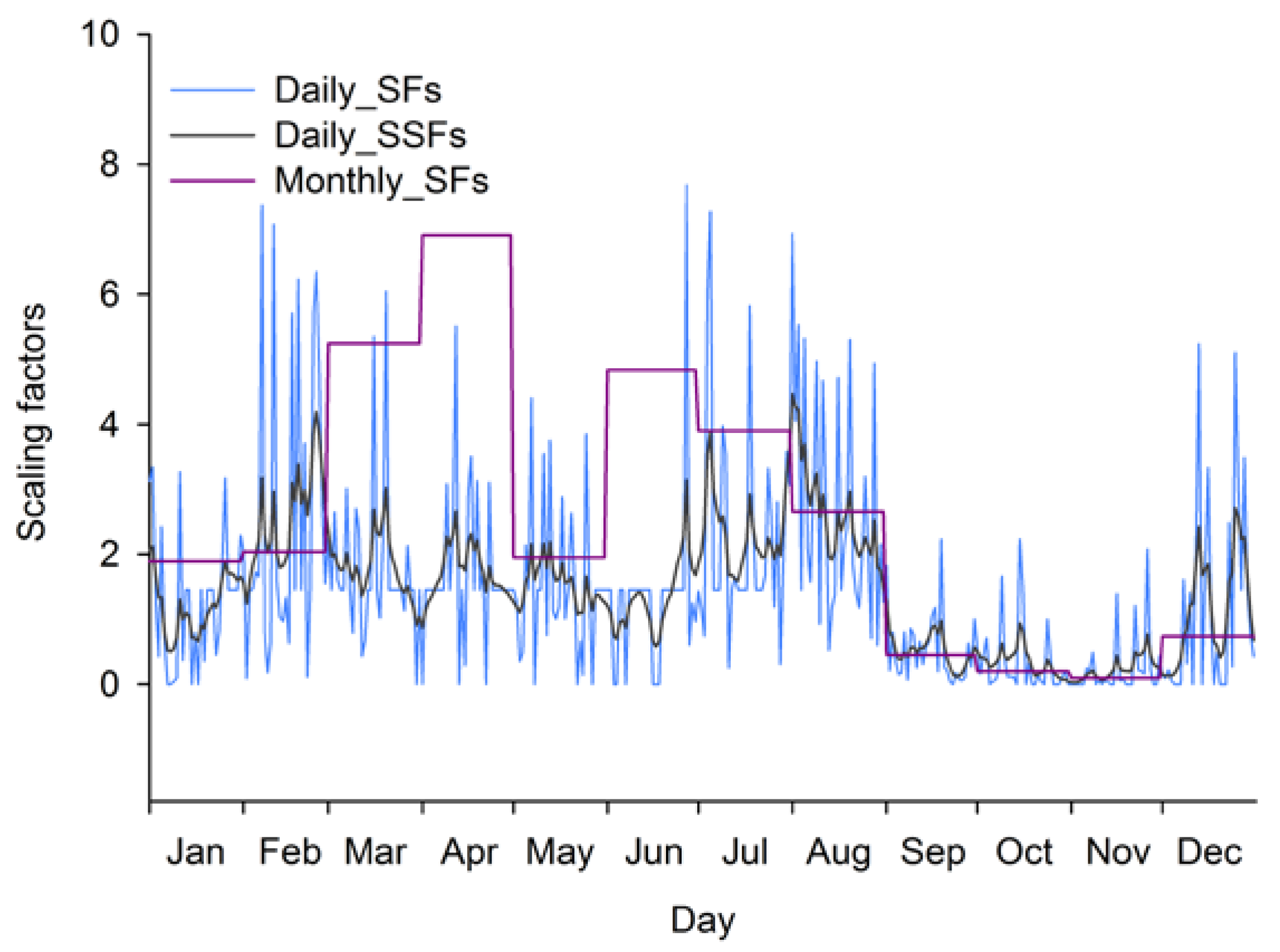
3.1. Precipitation Extended Linear Scaling (PELS) Method

Several bias-correction methods as mentioned above have been developed for correcting biases in GCM outputs. Each method has some advantages and drawbacks. The linear scaling or bias-correction methods are the simplest means to correct the outputs from GCMs. Due to their simplicity and fast application, these methods have widely been used in different parts of the world to correct GCM outputs, such as in [2,19,20,26,27,28]. Lately, these methods are not only applied to removing the biases of GCM outputs but also the biases of RCM outputs.

In the present study, an extended scaling method is proposed for correcting precipitation simulated from GCMs. This method is somehow similar to the method proposed by Mahmood and Jia [21] for temperature in the case of steps involved. However, this method differs in two ways from the method used for temperature: (1) calculating daily scaling factors for precipitation and (2) checking for outliers in daily scaling factors and adjusting the outliers before using them for precipitation correction. In the case of temperature, daily scaling factors are calculated by subtracting the mean daily observed temperature from GCM mean daily temperature. On the other hand, in the case of precipitation in this study, the DSFs were calculated by dividing the long period mean daily observed precipitation by GCM precipitation, as below:

$$P_{c\_GCM\_scen\_d}=P_{GCM\_scen\_d}\times \left(\frac{\overline{P_{obs\_cont\_d}}}{\overline{P_{GCM\_cont\_d}}}\right)$$

(1)

where $P_{c\_GCM\_scen\_d}$ is the corrected daily precipitation of GCMs for scenario period, for example 2021–2050 or 2041–2070; $P_{GCM\_scen\_d}$ is the daily scenario precipitation for the future periods; $\overline{P_{GCM\_cont\_d}}$ is the daily mean values of GCMs for the control period, for example 1971–2000. $\overline{P_{obs\_cont\_d}}$ describes mean daily precipitation observations for the control period.

In this study, 365 DSFs were calculated by GCM’s precipitation and observed precipitation, using this “$\left(\overline{P_{obs\_cont\_d}}/\overline{P_{GCM\_cont\_d}}\right)$”, instead of monthly means. It was observed during the calculation of SFs that some values were extraordinarily higher (as shown in Figure 3) because of the large difference between observed and GCM precipitation. The large fluctuations in daily SFs (shown in Figure 3) might be due to the small data period (1971–1985) because this kind of study requires long-term data. These outliers were detected using Tukey’s method [29] and adjusted with the mean monthly SF of that month. The mean SF for each month was calculated from the DSFs of that month after removing the outliers. After adjusting the detected outliers, the DSFs were also smoothed with a low pass filter (detail given in the next section). Finally, the DSFs were multiplied with daily GCM’s precipitation to get corrected precipitation. As with statistical downscaling methods, the main assumption of this method is that the scaling factors are temporally stationary. The number of SFs depends upon an annual cycle used for a GCM. For example, an annual cycle of 360 days is used in HadGEM2 but 365 days in GFDL. Therefore, different GCMs can have different DSFs depending on the number of days per year of a model. Since GCMs not only simulate different intensities of precipitation but also difference in frequency (number of precipitation days in specific period), this method, as with the original linear scaling (OLS) method, tends to correct the intensity not the frequency. Furthermore, the results can be improved by considering elevation difference between stations and GCM precipitation.

3.2. Evaluation of GCMs

Before any correction, the GCMs were evaluated by comparing them with the daily observed precipitation of 21 climate stations for the period of 1986–2000. Correlation coefficient (R), error between observed and GCM means (E_μ), root mean square error (RMSE), error between observed and GCM standard deviations (E_σ) were used for the evaluation of GCMs, as in [2,6,7]. Mean monthly precipitation of GCMs was also plotted against observations for evaluation purpose.

3.3. Evaluation of PELS Method

Before correcting the scenario time series of GCMs, PELS was evaluated using the historical observations of 21 stations and the GCM precipitation. PELS was also evaluated with OLS. The GCMs and observed precipitation datasets were divided into the following time periods: 1971–1985 and 1986–2000. The former period was considered as a control period, which was used to calculate DSFs and the later as a scenario period, which had to be corrected. The mean DSFs were obtained by using this part, $\left(\overline{P_{obs\_cont\_d}}/\overline{P_{GCM\_cont\_d}}\right)$, of Equation (1) for the control period. These DSFs were checked for outliers and replaced with mean values of the corresponding month, as explained above. These DSFs were attained separately for each precipitation gauge corresponding to the grid of GCMs, covering the site.

Before applying these DSFs directly into Equation (1), the triangle low pass filter, as described in Mahmood and Jia [21], was used to smooth the DSFs to reduce the noises. In this filter, more weight is assigned to the central value to reduce the effects of neighbor values, and thus this does not much affect the variance of data and extreme values in data.

For explanation, we calculated the DSFs and monthly scaling factor (MSFs) with both PELS and OLS, respectively, for the control period on the Jhelum precipitation gauge, and presented the figures graphically in Figure 4. This displays different DSFs (in case of magnitude) for each month in the case of PELS. However, only one scaling factor is shown in Figure 4 for all days of each month, which will reduce the daily variation in the corrected data. For example, in April (Figure 4), the DSFs ranged from 0.87 to 2.7 for different days, but the MSF for this month was 7.0 for all days of this month. This higher value was the result of only some big events that occurred during the whole period (1971–1985). Since the DSFs were checked for outliers and smoothed with a low pass filter, these big events did not have as much of an effect as in the case of PELS. Finally, the daily smooth scaling factors (DSSFs) were multiplied with the daily scenario precipitation of the GCMs to get the corrected precipitation time series for the scenario period (1986–2000), for all gauges.

The corrected precipitation by PELS was compared with observation for 1986–2000 using the above-mentioned statistical indicators (i.e., E_μ, RMSE, and E_σ) excluding the R because in this method we corrected the magnitude of the GCM precipitation and not the occurrence of precipitation. Therefore, it is obvious that R will not improve much. PELS was also evaluated with OLS to observe the improvement of this method over OLS. The corrected data was also compared with observed data graphically for evaluation purposes, as done in [2,6,7].

3.4. Projected Precipitation Changes

In this study, PELS was applied on the simulated data of 5 GCMs for 2041–2070 (2050s) under RCP8.5 and RCP2.6. The DSFs were obtained from the mean daily observed and GCM precipitation for the control period (1971–2000). Then these DSFs were checked for outliers and smoothed with the low pass filter. At the end, the daily precipitation simulated from 5 GCMs was corrected with the DSSFs for the period of the 2050s. The projected changes in precipitation with respect to the observed precipitation of control period were calculated for all the GCMs, as in [2,6,7].

4. Results and Discussion

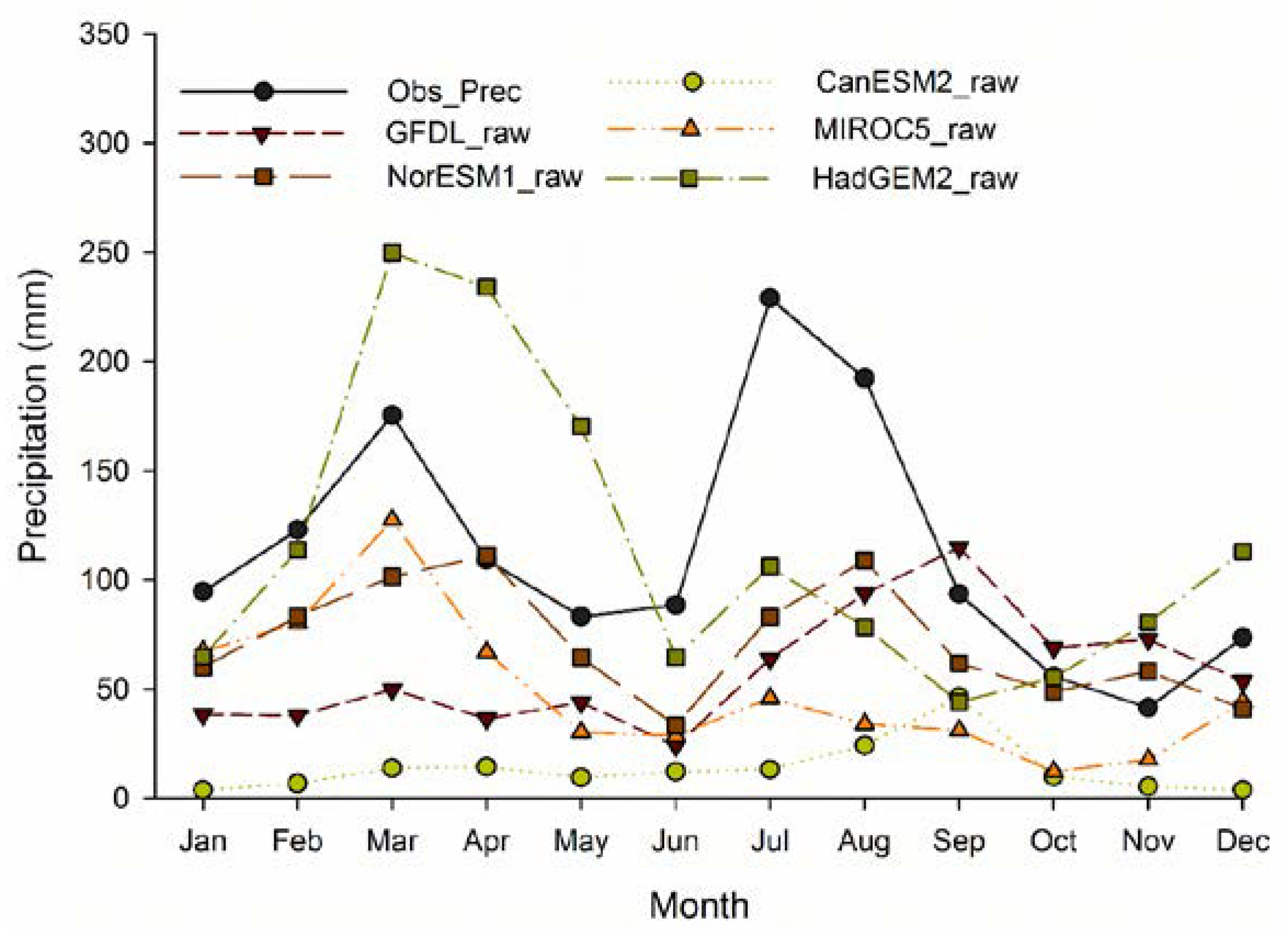
4.1. Evaluation of GCMs before Correction

The evaluation indicators calculated from daily raw precipitation of different GCMs with the observed precipitation are given in

Table 3. Evaluation of different GCMs with and without correction by PELS and OLS for 1986–2000 period, in the Jhelum River basin.

Indicators	CanESM2	GFDL	HadGEM2	MIROC5	NorESM1	Ensemble
Without correction
E_μ (%)	−86	−53	1	−57	−45	−48
E_σ (%)	−76	−50	−40	−69	−53	−57
RMSE (mm)	11	12	12	12	12	12
R	0.02	0.0001	0.002	0.01	0.02	0.01
Corrected with PELS
E_μ (%)	11	−2	−2	−4	−2	0.2
E_σ (%)	50	36	−33	36	20	21.8
RMSE (mm)	15	18	12	18	16	15.8
Corrected with OLS
E_μ (%)	−14	28	−2	23	9	8.8
E_σ (%)	44	115	−37	74	15	42.2
RMSE (mm)	19	25	12	21	17	18.8

E_μ error between GCM and observed means, E_σ error between GCM and observed standard deviations, R correlation coefficient, and RMSE root mean square error.

. All the GCMs presented poor results, e.g., R values ranged from 0.001 to 0.02 and RMSE from 11 to 12 mm/day. Similarly, the errors in predicting mean (E_μ) values ranged from −45% to −86%, and the errors in standard deviation (E_σ) ranged from −50% to −76%, which were so high and not acceptable. All the GCMs showed substantial underestimation in the values of predicting mean and standard deviation. HadGEM2 was the only model that showed good results in the case of predicting mean value, but it also failed to give good results in the case of other indicators, as with other GCMs. This limits the direct application of GCM precipitation in small basins.

To explore more detail about pattern comparison, the mean monthly GCM’s precipitation was plotted against the observed precipitation, and the graphs are shown in Figure 5. All the models completely failed to capture the variations of the observed precipitation and showed substantial underestimation in all months, except HadGEM2, which displayed substantial overestimation from March to May. Although HadGEM2 showed good results in the case of predicting mean values (Table 3), the model was still not acceptable because it overestimated from March to May and underestimated in other months (Figure 5). Thus, the correction of precipitation simulated by all the GCMs was required before using them in the basin.

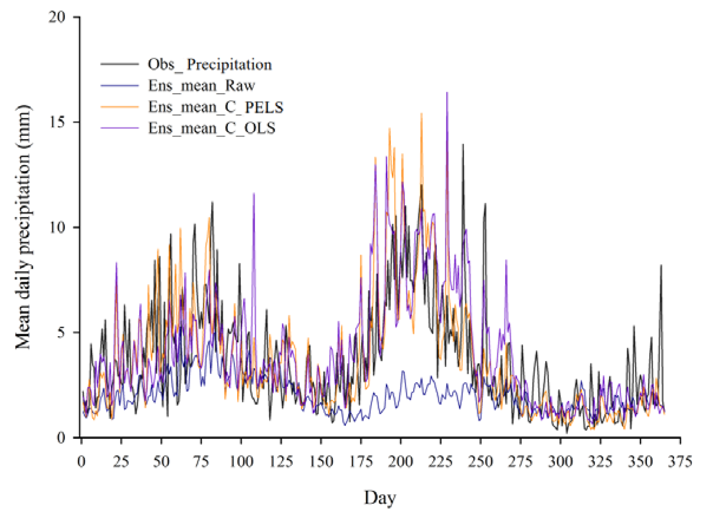
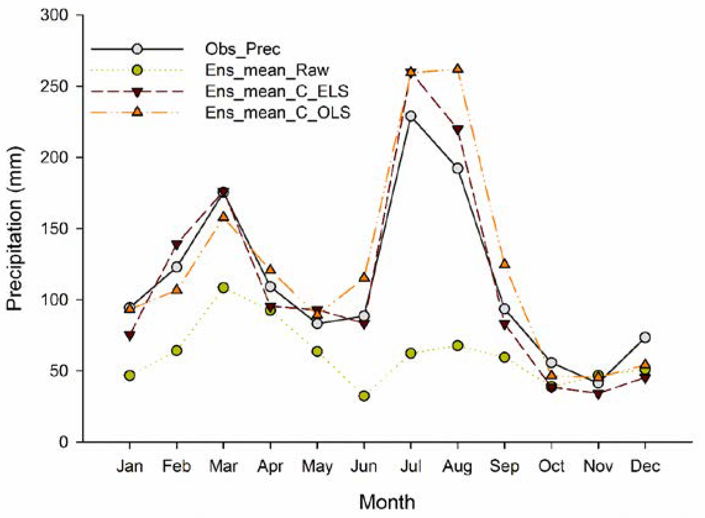
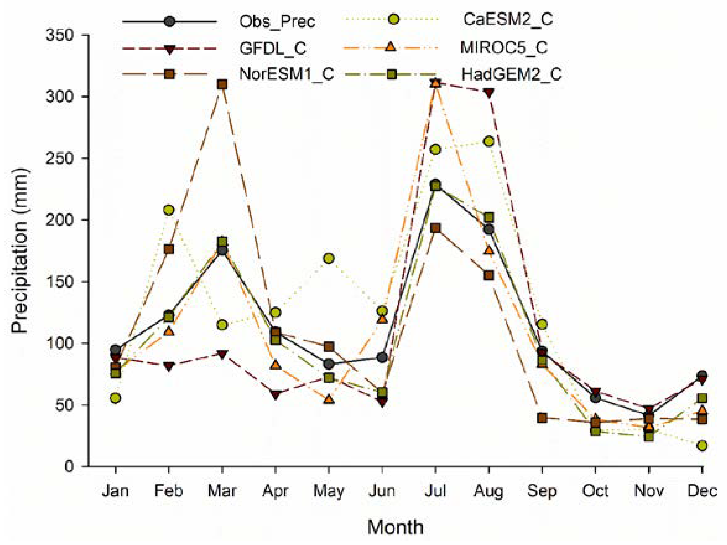
4.2. Evaluation of PELS Method

Table 3 displays the evaluation indicators calculated from the daily corrected precipitation by OLS and PELS and observed precipitation. Substantial improvement was observed in the case of predicting mean values. Absolute errors in prediction mean (E_μ) by PELS and OLS were reduced from 45–86% to 2–11% and 45–86% to 2–28%, respectively, for all the GCMs. Similarly, absolute errors in predicting standard deviation (E_σ) by PELS were also reduced from 40–76% to 20–50% for all the models. However, these values were increased after the correction with OLS for some GCMs: MIROC (74%) and GFDL (115%).

By comparison with PELS with OLS, PELS indicated better results in the case of predicting mean precipitation for all the GCMs. In case of predicting standard deviation, PELS performed better in 3 GCMs out of 5 GCMs. However, the values of RMSE by both methods were quite similar. For a detailed comparison between PELS and OLS, the mean daily precipitation of 5 GCMs (ensemble mean) corrected by both methods was graphically plotted against the observed daily precipitation and is shown in Figure 6, which shows that both methods can reproduce the daily patterns of the precipitation well better than the GCM ensemble, while they cannot regenerate daily variations exactly the same as the observed. This figure does not give a clearer picture of which method captured daily variations better.

Therefore, mean monthly precipitation of 5 GCMs (ensemble mean) corrected by both methods was graphically plotted against the mean monthly observed precipitation, as shown in Figure 7. The ensemble means by both methods captured the monthly variations of the observed precipitation as compared to the raw ensemble mean. However, OLS overestimated from April to September as compared to the PELS. On the whole, Figure 7 shows better presentation of PELS than OLS and much better than the raw ensemble mean. Table 3 also shows clear improvement of PELS over OLS, especially in the case of mean and standard deviations. PELS overestimated only 0.2% in the case of ensemble mean, while OLS overestimated 8.8%, and in the case of standard deviation, PELS overestimated 21.8% but OLS 42% (Table 3, last column).

For the evaluation of 5 GCMs after correction with PELS, the mean monthly precipitation of each model was plotted against the observed precipitation for the period of 1986–2000, and the plot is shown in Figure 8. After correction, all the GCMs followed the variations of observed precipitation although the models showed under- and overestimations in some months. NorESM1 overestimated from February to May, and after that it underestimated. Both peaks (the first small peak in March and the second big peak in July) were not completely captured by this model. It overestimated the small peak and underestimated the big peak. Conversely, the GFDL model underestimated the small peak and overestimated the big peak. In the case of months, it underestimated from January to June and overestimated during the rest of the months. Nonetheless, some months such as September to January were followed by this model. CanESM2 results were worse than all other GCMs; it did not follow the pattern of observed precipitation, as the other GCMs did. It was observed closely that MIROC5 and HadGEM2 followed the variations of observed precipitation. In addition, HadGEM2 also captured both peaks well. Although MIROC5 captured the small peak, the big peak was a little overestimated by the model. Thus, HadGEM2 performed relatively better than the other GCMs after the correction with PELS.

4.3. Projected Changes under RCPs

Table 4. Projected changes (%) in precipitation under RCP8.5 of different GCMs in the 2050s with respect to 1971–2000, in the Jhelum River basin.

Month	CanESM2	GFDL	MIROC5	NorESM1	HadGEM2	Average
Winter	1	118	−19	−37	−17	9
Spring	3	75	−18	−42	−1	4
Summer	4	−6	−50	−33	−25	−22
Fall	92	61	−15	−2	−57	16
Annual	10	50	−28	−31	−20	−4
March	−15	24	2	−34	15	−2
July	−9	−10	−61	−28	−27	−27
August	−21	−19	−69	−23	−38	−34

March, July, and August are the peak precipitation months.

shows seasonal, annual, and the peak month projected changes in the 2050s with respect to 1971–2000 under RCP8.5 in the Jhelum River basin. Most of the models projected decreasing precipitation (negative changes) in most of the seasons, and all models showed negative changes in the peak months except GFDL, MIROC5, and HadGEM2 in March. In the case of annual precipitation changes, GFDL and CanESM2 projected positive changes, with 10% and 50% increase, respectively. However, the other three models, i.e., MIROC5, HadGEM2, and NorESM1, projected an annual decrease of 28%, 31%, and 20%, respectively. The results of HadGEM2 and MIROC5 are more reliable because they showed best results during the evaluation. In the case of seasonal changes, four models showed negative changes in winter, two models in spring and fall, and all of the models in summer. In the case of ensemble mean (the last column), precipitation was projected to decrease by 22% in summer and projected to increase by 4%, 9%, and 16% in spring, winter, and fall, respectively. However, all models projected decrease in all the peak precipitation months, with an average decrease of 2%, 27%, and 34% in March, July, and August, respectively. It can be concluded that in the 2050s, the basin will receive about 4% less precipitation annually than the present, and in the peak months, this reduction can reach up to 34%.

Table 5. Projected changes (%) in precipitation under RCP2.6 of different GCMs in the 2050s with respect to 1971–2000, in the Jhelum River basin.

Month	CanESM2	GFDL	MIROC5	NorESM1	HadGEM2	Average
Winter	−2	72	−34	−28	−16	−2
Spring	25	68	−17	−30	9	11
Summer	13	−31	−58	−36	−35	−29
Fall	84	57	−57	−10	−48	5
Annual	21	32	−39	−27	−18	−6
March	28	38	−4	−24	18	11
July	−3	−48	−58	−31	−40	−36
August	−7	−21	−77	−31	−41	−36

March, July, and August are the peak precipitation months.

describes seasonal, annual, and the peak month changes in precipitation in the 2050s relative to 1971–2000 under RCP2.6. Three models MIROC5, NorESM1, and HadGEM2 showed negative changes in all seasons, annual, and peak months except HadGEM2 in spring and March. However, CanESM2 and GFDL showed mostly positive changes but negative changes in July and August. As the average of all models, an annual decrease of 6% was estimated in the basin, higher than RCP8.5. In winter and summer, precipitation was projected to decrease by 2% and 29%, respectively, and spring and fall showed increase in precipitation by 11% and 5%, respectively. similar to RCP8.5, in the peak months (July and August), all models showed decreasing precipitation by 36%, higher than RCP8.5. On the whole, on average, decreasing percentages under RCP2.6 were higher than RCP8.5.

5. Conclusions

Linear scaling (bias correction) methods are fast and simple techniques to reduce the biases from GCM outputs on local scales. In the present study, a linear scaling method known as precipitation extended linear scaling (PELS) was proposed to correct GCM precipitation. This method is basically the extension of the original linear scaling (OLS) method which is based on mean monthly scaling factors (MSFs). In this method, OLS is extended from monthly calculation of scaling factors to daily scaling factors. This means that in OLS, MSFs are used to correct the scenario data, but in the PELS method, mean daily scaling factors (DSFs) were used for correction. In addition, these DSFs were checked for outliers, replaced with mean values, and smoothed with a low pass filter before using them for the correction of the future precipitation.

For the evaluation of this method, the observed precipitation from 21 gauges and precipitation of five GCMs (i.e., GFDL, NorESM1, HadGEM2, MIROC5, and CanESM2) were collected for the transboundary Jhelum River basin in Pakistan and India. The observed data was collected from Pakistan and India and GCM data from CMIP5. Error in mean and in standard deviation relative to observed, root mean square error, and correlation coefficient were used for evaluation purposes. These GCMs were also evaluated with the observed precipitation for 1986–2000, without any correction. This showed that all the models underestimated the precipitation except HadGEM2, which overestimated in some months and underestimated in others. These models also showed lack of capability to capture the variations of observed precipitation, thereby limiting their direct application in the basin.

Before the application of this method for the correction of the future precipitation, the method was evaluated by correcting the precipitation data of 5 GCMs for the period of 1986–2000 and also compared with OLS. After correction with this method, a substantial improvement, of about 40–74%, was calculated in predicting mean values, and about 10–30% improvement was observed in predicting standard deviation. The comparison of OLS and PELS showed that PELS performed better than OLS both in the case of indicators and graphs.

After the evaluation of PELS, the future precipitation of 5 GCMs under RCP8.5 and RCP2.6 was corrected for 2041–2070, and the future changes in precipitation were calculated relative to the baseline period (1971–2000). According to the projected results, the Jhelum River basin will face an overall reduction in precipitation in the 2050s, with 4% and 6% annual decrease under RCP8.5 and RCP2.6, respectively. However, the summer season (monsoon) will be the most affected season in the future, which will face an average (all GCMs) reduction of 22% and 29% under RCP8.5 and RCP2.6, respectively, and even more severe reduction in precipitation in July and August under both scenarios, up to a 36% decrease. Therefore, if the climate of the world follows these RCPs, then there will be a severe reduction in precipitation in the Jhelum basin during peak months, which can create many problems for the economy of Pakistan because Pakistan’s economy is largely based on agriculture.

References

1. Fowler, H.J.; Blenkinsop, S.; Tebaldi, C. Linking climate change modelling to impacts studies: Recent advances in downscaling techniques for hydrological modelling. Int. J. Climatol. 2007, 27, 1547–1578. [Google Scholar] [CrossRef]
2. Mahmood, R.; Babel, M.S. Evaluation of SDSM developed by annual and monthly sub-models for downscaling temperature and precipitation in the Jhelum basin, Pakistan and India. Theor. Appl. Climatol. 2013, 113, 27–44. [Google Scholar] [CrossRef]
3. Zubler, E.M.; Fischer, A.M.; Fröb, F.; Liniger, M.A. Climate change signals of CMIP5 general circulation models over the Alps—Impact of model selection. Int. J. Climatol. 2015, 36, 3088–3104. [Google Scholar] [CrossRef]
4. Hay, L.E.; Wilby, R.L.; Leavesley, G.H. A comparison of delta change and downscaled GCM scenarios for three mountainous basins in the United States. J. Am. Water Resour. Assoc. 2000, 36, 387–397. [Google Scholar] [CrossRef]
5. Wetterhall, F.; Bárdossy, A.; Chen, D.; Halldin, S.; Xu, C.-Y. Daily precipitation-downscaling techniques in three Chinese regions. Water Resour. Res. 2006, 42, W11423. [Google Scholar] [CrossRef]
6. Chu, J.; Xia, J.; Xu, C.Y.; Singh, V. Statistical downscaling of daily mean temperature, pan evaporation and precipitation for climate change scenarios in Haihe River, China. Theor. Appl. Climatol. 2010, 99, 149–161. [Google Scholar] [CrossRef]
7. Huang, J.; Zhang, J.; Zhang, Z.; Xu, C.; Wang, B.; Yao, J. Estimation of future precipitation change in the Yangtze River basin by using statistical downscaling method. Stoch. Environ. Res. Risk Assess. 2011, 25, 781–792. [Google Scholar] [CrossRef]
8. Giorgi, F.; Hewitson, B.; Christensen, J.; Hulme, M.; Storch, V.H.; Whetton, P.; Jones, R.; Mearns, L.; Mearns, C.; Fu, C. Regional climate information-evaluation and projection. In Climate Change 2001: The Scientific Basis; Houghton, J.T., Ding, Y., Griggs, D.J., Noguer, M., Dai, X., Maskell, K., Eds.; Cambridge University Press: Cambridge, UK, 2001; pp. 585–629. [Google Scholar]
9. Hay, L.E.; Clark, M.P. Use of statistically and dynamically downscaled atmospheric model output for hydrologic simulations in three mountainous basins in the western United States. J. Hydrol. 2003, 282, 56–75. [Google Scholar] [CrossRef]
10. Wilby, R.L.; Dawson, C.W.; Barrow, E.M. Sdsm—A decision support tool for the assessment of regional climate change impacts. Environ. Model. Softw. 2002, 17, 145–157. [Google Scholar] [CrossRef]
11. Hessami, M.; Gachon, P.; Ouarda, T.B.M.J.; St-Hilaire, A. Automated regression-based statistical downscaling tool. Environ. Model. Softw. 2008, 23, 813–834. [Google Scholar] [CrossRef]
12. Semenov, M.A.; Barrow, E.M. Use of a stochastic weather generator in the development of climate change scenarios. Clim. Chang. 1997, 33, 397–414. [Google Scholar] [CrossRef]
13. Maraun, D. Bias correction, quantile mapping, and downscaling: Revisiting the inflation issue. J. Clim. 2013, 26, 2137–2143. [Google Scholar] [CrossRef]
14. Fang, G.H.; Yang, J.; Chen, Y.N.; Zammit, C. Comparing bias correction methods in downscaling meteorological variables for a hydrologic impact study in an arid area in China. Hydrol. Earth Syst. Sci. 2015, 19, 2547–2559. [Google Scholar] [CrossRef] [Green Version]
15. Teutschbein, C.; Seibert, J. Bias correction of regional climate model simulations for hydrological climate-change impact studies: Review and evaluation of different methods. J. Hydrol. 2012, 456–457, 12–29. [Google Scholar] [CrossRef]
16. Chen, J.; Brissette, F.P.; Chaumont, D.; Braun, M. Finding appropriate bias correction methods in downscaling precipitation for hydrologic impact studies over North America. Water Resour. Res. 2013, 49, 4187–4205. [Google Scholar] [CrossRef]
17. Xu, C.-Y. From GCMs to river flow: A review of downscaling methods and hydrologic modelling approaches. Prog. Phys. Geogr. 1999, 23, 229–249. [Google Scholar] [CrossRef]
18. Santer, B.D.; Wigley, T.M.L.; Schlesinger, M.E.; Mitchell, J.F.B. Developing Climate Scenarios from Equilibrium GCM; Max Planck Institute for Meteorology: Hamburg, Germany, 1990; p. 29. [Google Scholar]
19. Ouyang, F.; Zhu, Y.; Fu, G.; Lü, H.; Zhang, A.; Yu, Z.; Chen, X. Impacts of climate change under CMIP5 RCP scenarios on streamflow in the huangnizhuang catchment. Stoch. Environ. Res. Risk Assess. 2015, 29, 1781–1795. [Google Scholar] [CrossRef]
20. Mpelasoka, F.S.; Chiew, F.H.S. Influence of rainfall scenario construction methods on runoff projections. J. Hydrometeorol. 2009, 10, 1168–1183. [Google Scholar] [CrossRef]
21. Mahmood, R.; Jia, S. An extended linear scaling method for downscaling temperature and its implication in the Jhelum River basin, Pakistan, and India, using CMIP5 GCMs. Theor. Appl. Climatol. 2017, 130, 725–734. [Google Scholar] [CrossRef]
22. Archer, D.R.; Fowler, H.J. Using meteorological data to forecast seasonal runoff on the River Jhelum, Pakistan. J. Hydrol. 2008, 361, 10–23. [Google Scholar] [CrossRef]
23. Taylor, K.E.; Stouffer, R.J.; Meehl, G.A. An overview of CMIP5 and the experiment design. Bull. Am. Meteorol. Soc. 2011, 93, 485–498. [Google Scholar] [CrossRef]
24. Prasanna, V. Regional climate change scenarios over South Asia in the CMIP5 coupled climate model simulations. Meteorol. Atmos. Phys. 2015, 127, 561–578. [Google Scholar] [CrossRef]
25. Babar, Z.; Zhi, X.-F.; Fei, G. Precipitation assessment of Indian summer monsoon based on CMIP5 climate simulations. Arab. J. Geosci. 2015, 8, 4379–4392. [Google Scholar] [CrossRef]
26. Piani, C.; Haerter, J.; Coppola, E. Statistical bias correction for daily precipitation in regional climate models over Europe. Theor. Appl. Climatol. 2010, 99, 187–192. [Google Scholar] [CrossRef]
27. Akhtar, M.; Ahmad, N.; Booij, M.J. Use of regional climate model simulations as input for hydrological models for the Hindukush-Karakorum-Himalaya region. Hydrol. Earth Syst. Sci. 2009, 13, 1075–1089. [Google Scholar] [CrossRef]
28. Salzmann, N.; Frei, C.; Vidale, P.-L.; Hoelzle, M. The application of Regional Climate Model output for the simulation of high-mountain permafrost scenarios. Glob. Planet. Chang. 2007, 56, 188–202. [Google Scholar] [CrossRef]
29. Tukey, J.W. Exploratory Data Analysis, 1st ed.; Pearson: London, UK, 1977. [Google Scholar]
Figure 1. Location map of the study area, the Jhelum River basin, showing precipitation gauges.
Atmosphere 09 00160 g001
Figure 2. GCM grids coving the Jhelum River basin.
Atmosphere 09 00160 g002
Figure 3. Scaling factors calculated for June to September at Astor climate station with (small plot) and without (large plot) outlier check and smoothed with low pass filter, for the period of 1971–1986.
Atmosphere 09 00160 g003
Figure 4. Scaling factors calculated by the PELS method (blue line without smoothing and black line with smoothing) and original linear scaling (red line) at Jhelum site for 1971–1985 period.
Atmosphere 09 00160 g004
Figure 5. Comparison between observed and GCM raw precipitation for 1986–2000, in the Jhelum River basin.
Atmosphere 09 00160 g005
Figure 6. Comparison of daily mean observed precipitation against raw GCM precipitation (ensemble mean of five GCMs), corrected precipitation with PELS, and corrected precipitation with OLS.
Atmosphere 09 00160 g006
Figure 7. Observed precipitation against ensemble mean of five GCMs taken from raw GCM data, corrected with PELS, and corrected with OLS.
Atmosphere 09 00160 g007
Figure 8. Comparison between observed and GCM precipitation corrected by the PELS method for 1986–2000 in the Jhelum River basin.
Atmosphere 09 00160 g008