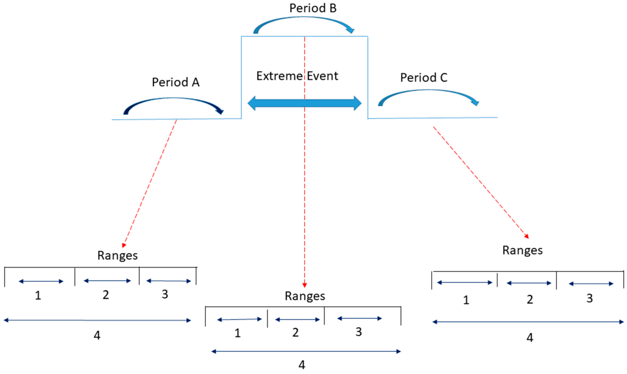
Figure 1.
Schematic representation of the methodological steps followed in this study.
Figure 1.
Schematic representation of the methodological steps followed in this study.
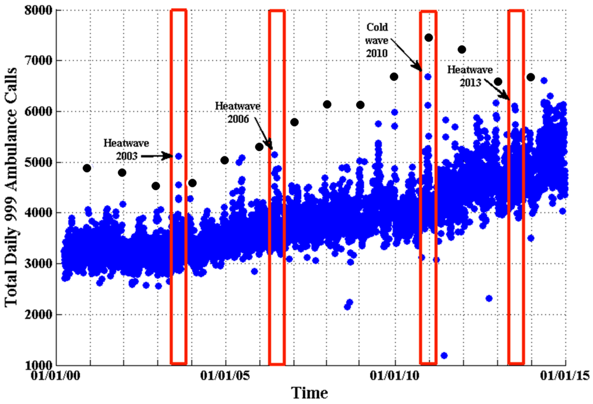
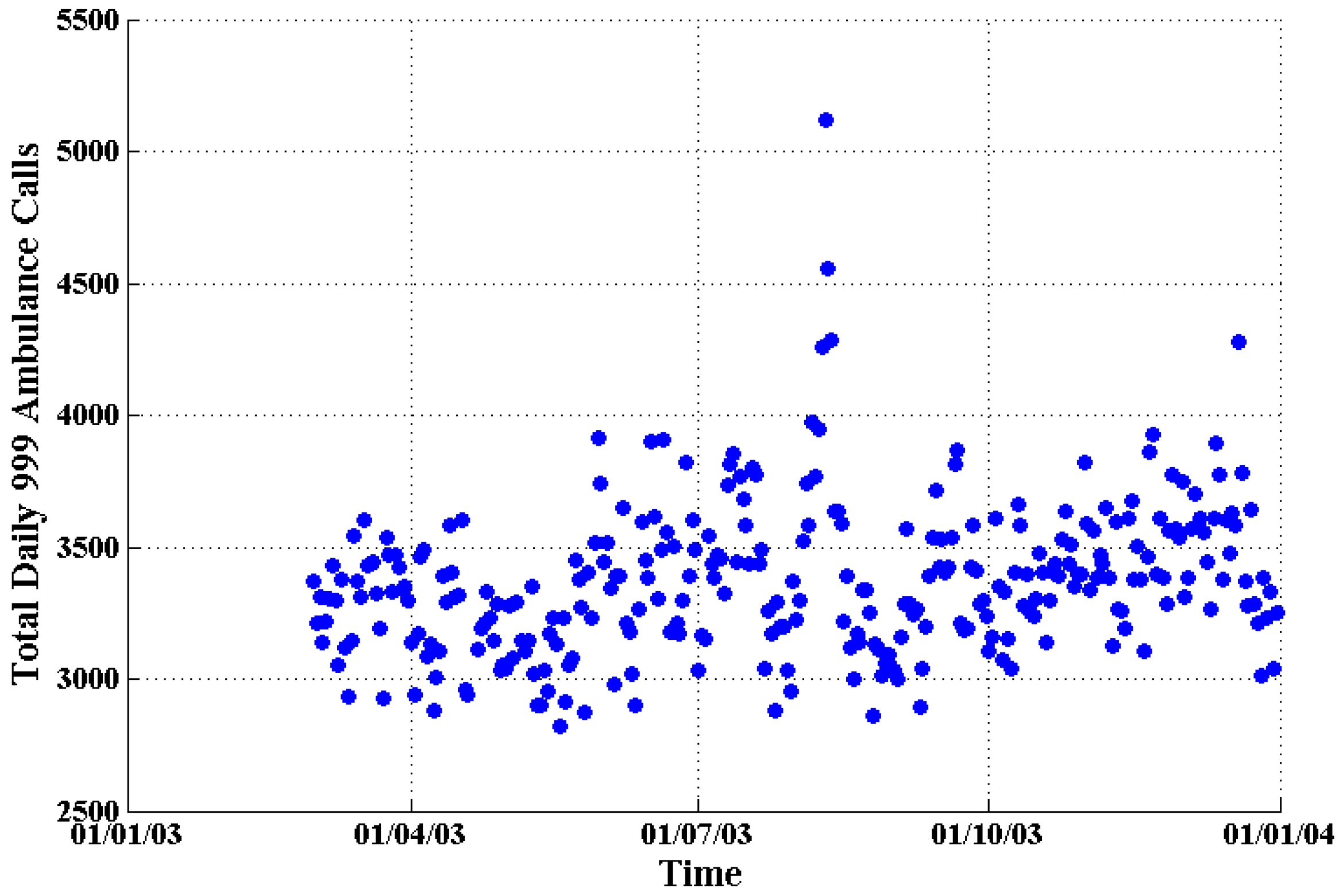
Figure 2.
The daily total number of 999 emergency ambulance incidents (calls—blue dots) in London from 1 April 2000 to 31 December 2014. The red rectangles delimit the four extreme temperature episodes which we study in this paper. Seasonal peaks which are the spikes on the 1 January each year are marked with black dots (see text above).
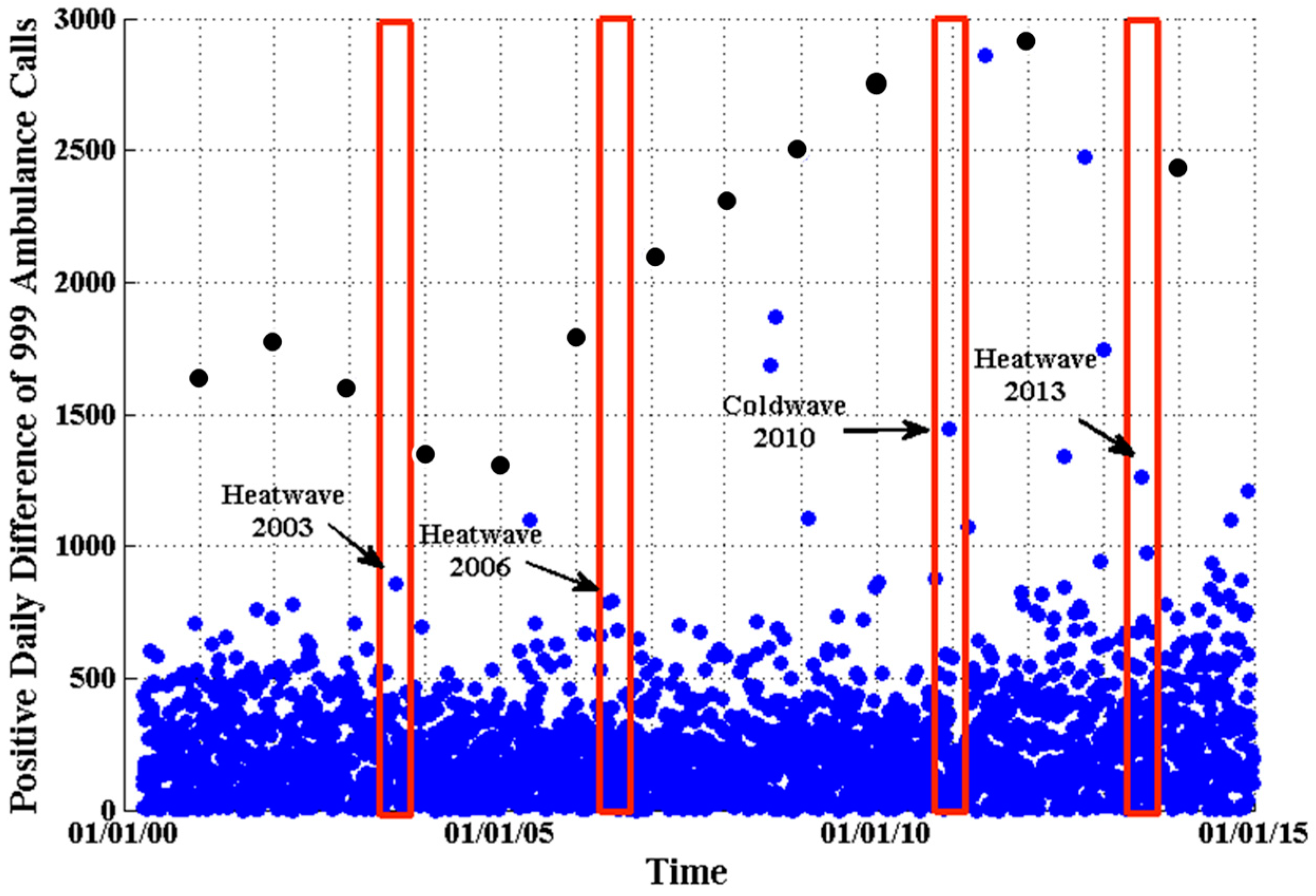
Figure 3.
The positive daily difference of the total number of 999 emergency ambulance calls (blue dots) in London from 1 April 2000 to 31 December 2014. The red rectangles delimit the four extreme temperature episodes which we study in this paper. Seasonal peaks which are the spikes on the 1 January each year are marked with black dots (see text above).
Figure 4.
The daily total number of 999 emergency ambulance calls (blue dots) in London from 1 July 2010 to 31 May 2011.
Figure 4.
The daily total number of 999 emergency ambulance calls (blue dots) in London from 1 July 2010 to 31 May 2011.
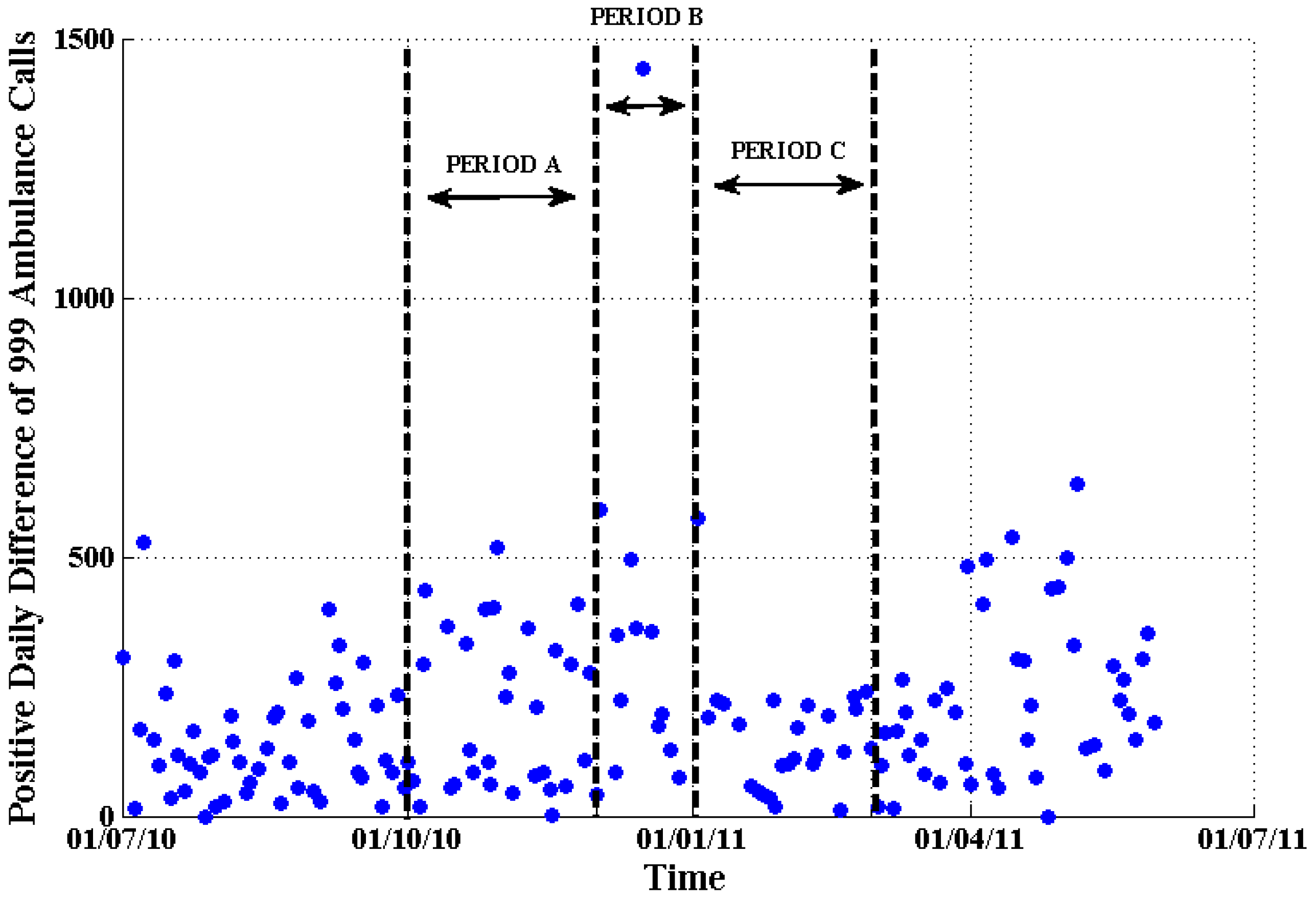
Figure 5.
The positive daily difference of calls of 999 emergency ambulance incidents (blue dots) in London from 1 July 2010 to 31 May 2011. The dataset is divided into three periods. Period A corresponds to the period before the extreme temperature, Period B is the extreme temperature period and Period C is after the extreme temperature.
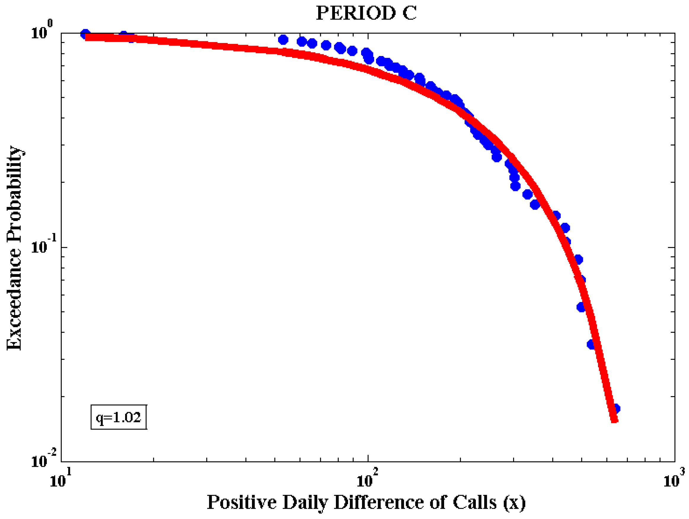
Figure 6.
Log–log plot of the exceedance probability distribution function. The dataset (blue dots) and the Tsallis fitting curve (Equation (1), red line) for period C of the 2010 cold wave. The q value is calculated equal to 1.02.
Figure 6.
Log–log plot of the exceedance probability distribution function. The dataset (blue dots) and the Tsallis fitting curve (Equation (1), red line) for period C of the 2010 cold wave. The q value is calculated equal to 1.02.
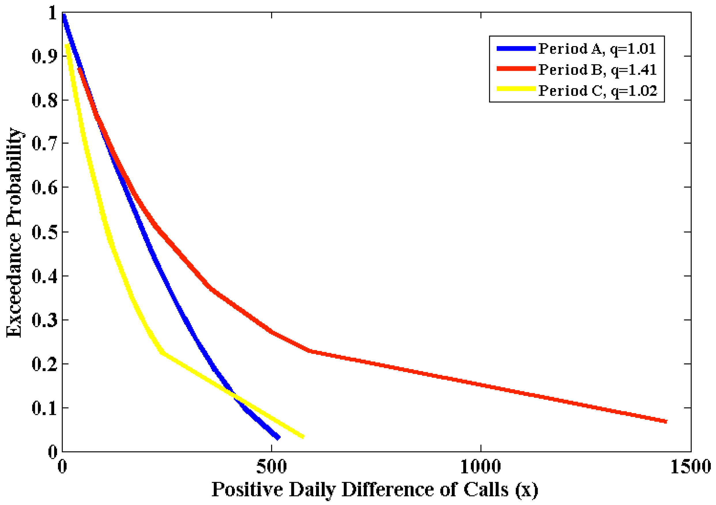
Figure 7.
The exceedance probability distribution function corresponding to each period. It should be noted that the axis in this plot is not in logarithmic scale as in
Figure 6.
Figure 7.
The exceedance probability distribution function corresponding to each period. It should be noted that the axis in this plot is not in logarithmic scale as in
Figure 6.
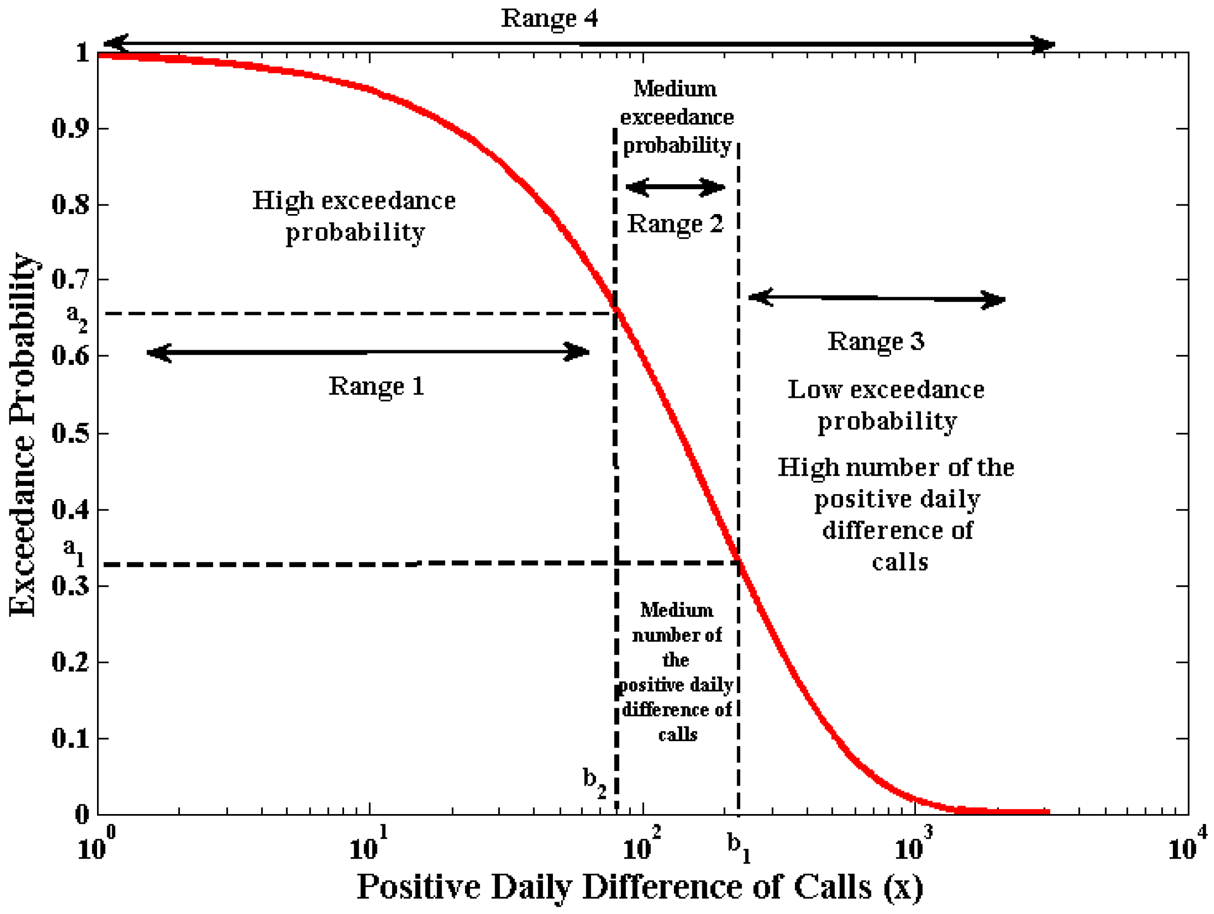
Figure 8.
The partition of the positive daily difference of calls into three ranges of the exceedance probability (red line), i.e., high, medium and low exceedance probability, for the whole dataset, in London from 1 July 2010 to 31 May 2011. The x-axis is in logarithmic scale.
Figure 8.
The partition of the positive daily difference of calls into three ranges of the exceedance probability (red line), i.e., high, medium and low exceedance probability, for the whole dataset, in London from 1 July 2010 to 31 May 2011. The x-axis is in logarithmic scale.
Figure 9.
The daily total number of 999 emergency ambulance calls (blue dots) in London from 1 March 2003 to 31 December 2003.
Figure 9.
The daily total number of 999 emergency ambulance calls (blue dots) in London from 1 March 2003 to 31 December 2003.
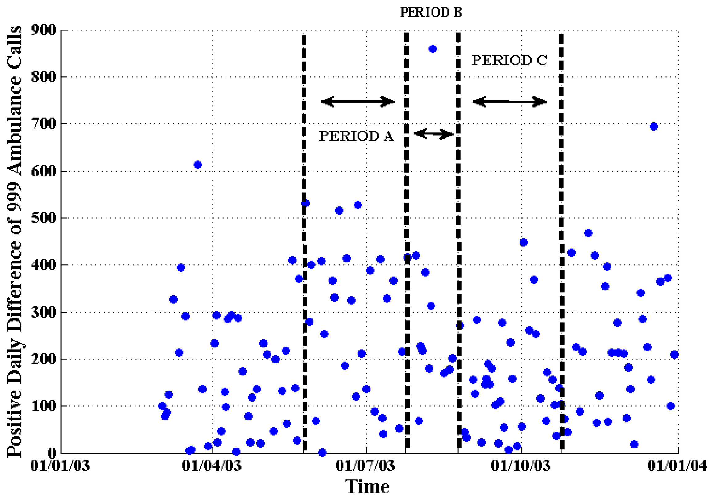
Figure 10.
The positive daily difference of calls of 999 emergency ambulance incidents (blue dots) in London from 1 March 2003 to 31 December 2003.
Figure 10.
The positive daily difference of calls of 999 emergency ambulance incidents (blue dots) in London from 1 March 2003 to 31 December 2003.
Figure 11.
The daily total number of 999 emergency ambulance calls (blue dots) in London from 1 February 2006 to 30 November 2006.
Figure 11.
The daily total number of 999 emergency ambulance calls (blue dots) in London from 1 February 2006 to 30 November 2006.
Figure 12.
The positive daily difference of calls of 999 emergency ambulance calls (blue dots) in London from 1 February 2006 to 30 November 2006.
Figure 12.
The positive daily difference of calls of 999 emergency ambulance calls (blue dots) in London from 1 February 2006 to 30 November 2006.
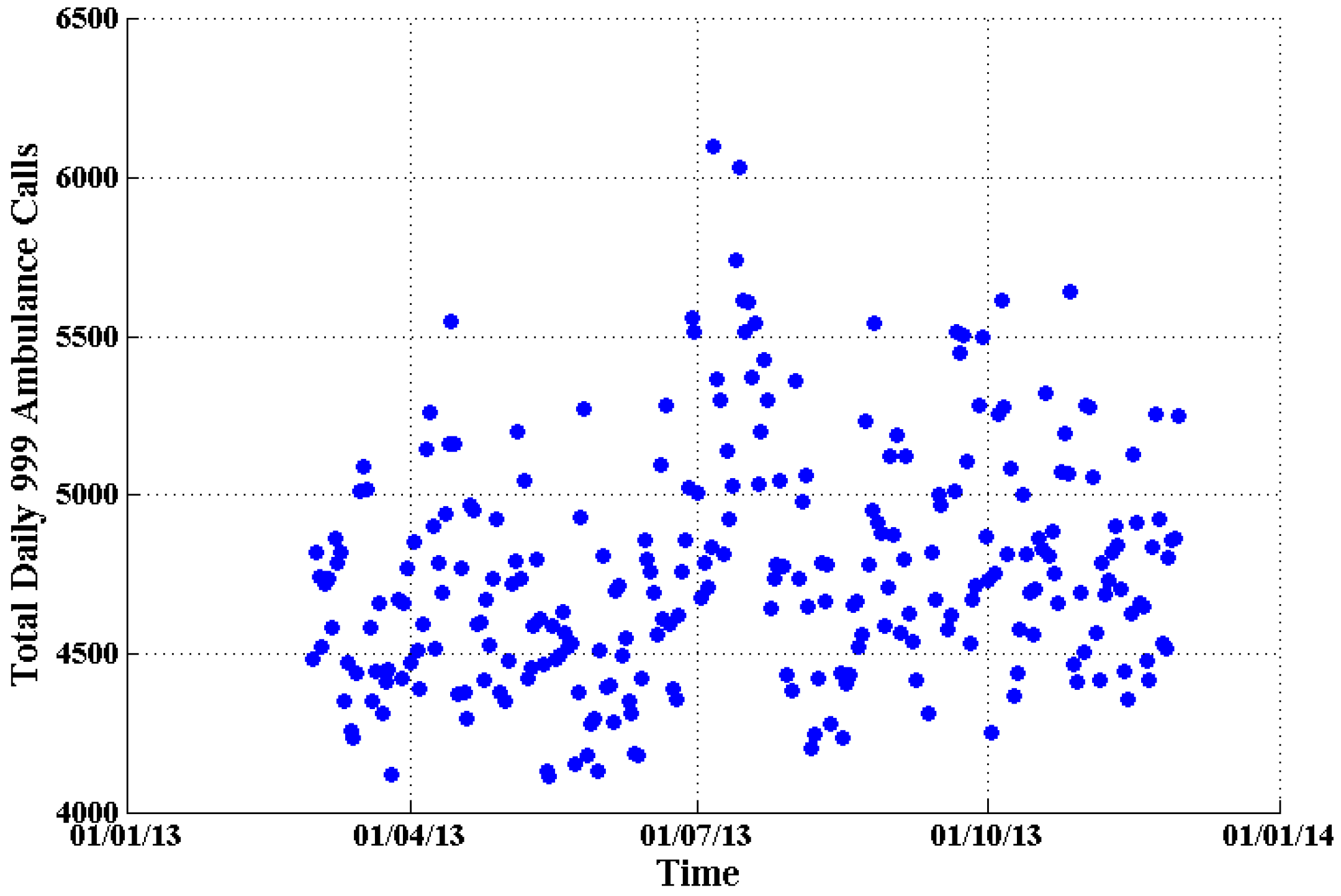
Figure 13.
The daily total number of 999 emergency ambulance calls (blue dots) in London from 1 March 2013 to 30 November 2013.
Figure 13.
The daily total number of 999 emergency ambulance calls (blue dots) in London from 1 March 2013 to 30 November 2013.
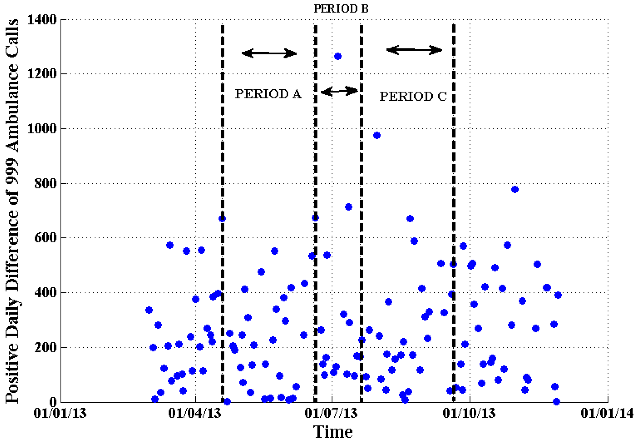
Figure 14.
The positive daily difference of calls of 999 emergency ambulance calls (blue dots) in London from 1 March 2013 to 30 November 2013.
Figure 14.
The positive daily difference of calls of 999 emergency ambulance calls (blue dots) in London from 1 March 2013 to 30 November 2013.
Table 1.
Selected periods of study and the associated number of days for four extreme temperature episodes.
Table 1.
Selected periods of study and the associated number of days for four extreme temperature episodes.
| Extreme Temperature Episode | Selected Period | Number of Days |
|---|
| Cold spell in December 2010 | 1 October 2010–28 February 2011 | 151 |
| Heat wave in August 2003 | 25 May 2003–24 October 2003 | 153 |
| Heat wave in July 2006 | 15 April 2006–16 September 2006 | 155 |
| Heat wave in July 2013 | 19 April 2013–21 September 2013 | 156 |
Table 2.
The estimated q value and Tsallis expected value for the four ranges of each period.
Table 2.
The estimated q value and Tsallis expected value for the four ranges of each period.
| Period | q | Range 1 (Tsallis Mean Value) | Range 2 (Tsallis Mean Value) | Range 3 (Tsallis Mean Value) | Range 4 (Tsallis Mean Value) |
|---|
| A | | | | | |
| 1 October 2010–30 November 2010 | 1.01 | 46 | 28 | 42 | 116 |
| B | | | | | |
| 1 December 2010–31 December 2010 | 1.41 | 37 | 72 | 98 | 207 |
| C | | | | | |
| 1 January 2011–28 February 2011 | 1.02 | 14 | 43 | 45 | 102 |
Table 3.
Sensitivity analysis. The estimated q value and Tsallis expected value for the four ranges of each period when Period B is set to last 2 months.
Table 3.
Sensitivity analysis. The estimated q value and Tsallis expected value for the four ranges of each period when Period B is set to last 2 months.
| Period | q | Range 1 (Tsallis Mean Value) | Range 2 (Tsallis Mean Value) | Range 3 (Tsallis Mean Value) | Range 4 (Tsallis Mean Value) |
|---|
| A | | | | | |
| 15 September 2010–14 November 2010 | 1.01 | 50 | 26 | 34 | 110 |
| B | | | | | |
| 15 November 2010–15 January 2011 | 1.43 | 25 | 82 | 86 | 193 |
| C | | | | | |
| 16 January 2011–15 March 2011 | 1.02 | 14 | 40 | 41 | 95 |
Table 4.
The estimated q value and Tsallis expected value for each range of each period.
Table 4.
The estimated q value and Tsallis expected value for each range of each period.
| Period | q | Range 1 (Tsallis Mean Value) | Range 2 (Tsallis Mean Value) | Range 3 (Tsallis Mean Value) | Range 4 (Tsallis Mean Value) |
|---|
| A | | | | | |
| 25 May 2003–24 July 2003 | 1.01 | 25 | 60 | 45 | 130 |
| B | | | | | |
| 25 July 2003–24 August 2003 | 1.10 | 47 | 80 | 100 | 227 |
| C | | | | | |
| 25 August 2003–24 October 2003 | 1.01 | 17 | 49 | 28 | 94 |
Table 5.
The estimated q value and Tsallis expected value for the four ranges of each period.
Table 5.
The estimated q value and Tsallis expected value for the four ranges of each period.
| Period | q | Range 1 (Tsallis Mean Value) | Range 2 (Tsallis Mean Value) | Range 3 (Tsallis Mean Value) | Range 4 (Tsallis Mean Value) |
|---|
| A | | | | | |
| 15 April 2006–14 June 2006 | 1.01 | 18 | 39 | 33 | 90 |
| B | | | | | |
| 15 June 2006–15 July 2006 | 1.38 | 27 | 60 | 61 | 148 |
| C | | | | | |
| 16 July 2006–16 September 2006 | 1.04 | 10 | 34 | 33 | 77 |
Table 6.
The estimated q value and Tsallis expected value for the four ranges of each period.
Table 6.
The estimated q value and Tsallis expected value for the four ranges of each period.
| Period | q | Range 1 (Tsallis Mean Value) | Range 2 (Tsallis Mean Value) | Range 3 (Tsallis Mean Value) | Range 4 (Tsallis Mean Value) |
|---|
| A | | | | | |
| 19 March 2013–19 June 2013 | 1.01 | 21 | 54 | 50 | 125 |
| B | | | | | |
| 20 June 2013–20 July 2013 | 1.24 | 63 | 62 | 77 | 202 |
| C | | | | | |
| 21 July 2013–26 September 2013 | 1.03 | 22 | 60 | 52 | 134 |
Table 7.
The standard and Tsallis values, and the additional Tsallis value due to extreme weather (Range) 3 for the four case studies (extreme weather periods).
Table 7.
The standard and Tsallis values, and the additional Tsallis value due to extreme weather (Range) 3 for the four case studies (extreme weather periods).
| Period B | Standard Mean | Tsallis Mean (Mean Value of Calls for Range 4) | Additional Tsallis Mean at Extreme Temperature (Mean Values of Calls for Range 3) |
|---|
| Cold wave: December 2010 | 348 | 207 | 98 |
| Heat wave: August 2003 | 303 | 227 | 100 |
| Heat wave: July 2006 | 195 | 148 | 61 |
| Heat wave: July 2013 | 338 | 202 | 77 |
Table 8.
The exceedance probability for various thresholds of the positive daily difference of calls.
Table 8.
The exceedance probability for various thresholds of the positive daily difference of calls.
| Period B | Exceedance Probability for |
|---|
| Positive Daily Difference of Calls ≥ 100 | Positive Daily Difference of Calls ≥ 200 | Positive Daily Difference of Calls ≥ 400 | Positive Daily Difference of Calls ≥ 700 |
|---|
| Cold wave: December 2010 | 0.72 | 0.54 | 0.34 | 0.2 |
| Heat wave: August 2003 | 0.76 | 0.56 | 0.31 | 0.15 |
| Heat wave: July 2006 | 0.59 | 0.37 | 0.16 | 0.09 |
| Heat wave: July 2013 | 0.74 | 0.56 | 0.34 | 0.17 |
Table 9.
The expected number of the positive daily difference of calls during a hypothetical seven-day extreme temperature period using the standard and Tsallis means for comparison (first and second rows). The third row gives the expected number of the positive daily difference of additional calls during the seven-day extreme temperature period relative to a normal seven-day period.
| Seven-Day Period of Extreme Temperature |
|---|
| Standard Mean | 1365–2436 is the spread of the total number of the positive daily difference of calls during the seven-day period of extreme temperature. |
| Tsallis Mean (Range 4) | 1036–1589 is the spread of the total number of the positive daily difference of calls during the seven-day period of extreme temperature. |
| Additional Tsallis mean at extreme temperature (Range 3) | 427–700 is the spread of the positive daily difference of additional calls due to the seven-day extreme temperature compared to a normal temperature period. |


