Simulation of a Large Wildfire in a Coupled Fire-Atmosphere Model


1
SPE—Sciences Pour l’Environnement, Université de Corse, CNRS, Campus Grimaldi, 20250 Corte, France
2
LA—Laboratoire D’Aérologie, Université de Toulouse, CNRS, UPS, 14 Avenue Edouard Belin, 31400 Toulouse, France
3
CNRM—Centre National de Recherches Météorologiques, Météo-France, CNRS, 42 Avenue Coriolis, 31057 Toulouse, France
*
Author to whom correspondence should be addressed.
Atmosphere 2018, 9(6), 218; https://doi.org/10.3390/atmos9060218
Submission received: 6 April 2018
/
Revised: 24 May 2018
/
Accepted: 28 May 2018
/
Published: 7 June 2018
(This article belongs to the Special Issue Fire and the Atmosphere)
Abstract
:The Aullene fire devastated more than 3000 ha of Mediterranean maquis and pine forest in July 2009. The simulation of combustion processes, as well as atmospheric dynamics represents a challenge for such scenarios because of the various involved scales, from the scale of the individual flames to the larger regional scale. A coupled approach between the Meso-NH (Meso-scale Non-Hydrostatic) atmospheric model running in LES (Large Eddy Simulation) mode and the ForeFire fire spread model is proposed for predicting fine- to large-scale effects of this extreme wildfire, showing that such simulation is possible in a reasonable time using current supercomputers. The coupling involves the surface wind to drive the fire, while heat from combustion and water vapor fluxes are injected into the atmosphere at each atmospheric time step. To be representative of the phenomenon, a sub-meter resolution was used for the simulation of the fire front, while atmospheric simulations were performed with nested grids from 2400-m to 50-m resolution. Simulations were run with or without feedback from the fire to the atmospheric model, or without coupling from the atmosphere to the fire. In the two-way mode, the burnt area was reproduced with a good degree of realism at the local scale, where an acceleration in the valley wind and over sloping terrain pushed the fire line to locations in accordance with fire passing point observations. At the regional scale, the simulated fire plume compares well with the satellite image. The study explores the strong fire-atmosphere interactions leading to intense convective updrafts extending above the boundary layer, significant downdrafts behind the fire line in the upper plume, and horizontal wind speeds feeding strong inflow into the base of the convective updrafts. The fire-induced dynamics is induced by strong near-surface sensible heat fluxes reaching maximum values of 240 . The dynamical production of turbulent kinetic energy in the plume fire is larger in magnitude than the buoyancy contribution, partly due to the sheared initial environment, which promotes larger shear generation and to the shear induced by the updraft itself. The turbulence associated with the fire front is characterized by a quasi-isotropic behavior. The most active part of the Aullene fire lasted 10 h, while 9 h of computation time were required for the 24 million grid points on 900 computer cores.
1. Introduction
Although a natural process in most part of the world, wildland fires represent a constant threat wherever there exists a possible interface with human activities. A large number of tightly-coupled physical phenomena interact in the development of a large wildfire. Temperature increase in the fuel generates pyrolysis gases, the composition of which depends on the vegetation, and which can blaze. The intense heat release can dramatically modify the local meteorology, generating strong local convective motion and fire-induced winds, that in turn modify the fire front dynamics and drive the fire propagation [1]. To simulate wildland fire, the fire front propagation must be solved at the scale of a few meters to precisely take into account wind, slope, humidity and obstacles (road, rocks). Eventually, fire-atmosphere interactions with the local motions need to be taken into account to properly represent the composition, density, structure and transport of the plume.
Nevertheless, simulating large wildland fires requires choosing between the complexity of the code, data availability, the speed at which the result must be obtained and the computational framework. The variety of models thus ranges from physically-detailed, fire/atmosphere coupled and computationally-intensive (and limited to relatively small fires) models such as FIRETEC [2], WFDS [3] or FIRESTAR [4,5] to empirical, uncoupled (forced wind field) models such as FARSITE [6] that are adapted to provide rapid simulation of very large wildfires. As an intermediate trade-off, approaches coupling a 2D-surface fire propagation model with a mesoscale atmospheric model [7,8,9] have shown their ability to capture some of the complex phenomena occurring in large fires while still being adapted to a real-time response.
This last approach is developed in this study, which focuses on testing the ability of these coupled fire-atmosphere models to represent micro-scale atmospheric and fire front effects on a real and large observed fire case. Numerical fire/atmosphere coupling has already undergone numerous studies, starting from the static fire simulations of [10] to the pioneering works of [7,11] where a simplified model of [12] fire spread was coupled to the atmospheric model of [13]. More recently, the original Clark/Coen model evolved to the CAWFE model [14], while efforts at extending the WRF weather forecasting model [15] have resulted in the WRF/fire module [8], widely used even at the scale of large fires (several square kilometers [16,17,18,19]).
A similar system is used here, based on the atmospheric Meso-NH model [20,21] interactively coupled with the ForeFire fire spread model [22]. Specifically, the fire model is different from the [23] model used in other approaches taking into account the effects of wind and slope through coefficients experimentally fitted to wind values “as if the fire was not there”. Moreover, although large wildfires remain an objective, specific numerical methods were developed so that all phenomena could be simulated at a resolution close to their characteristic scale.
The target case study is decomposed into four nested domains ranging from 2.4-km to 50-m resolution, allowing one to explore the local to the regional impact of a large wildfire in an interactive fire-atmosphere coupling. Fire front is integrated at the scale of thermal transfer (sub-meter), fuel consumption at the resolution of the vegetation database (5 m), local atmosphere and winds at the resolution of the convective structures above the fire front (50 m) and smoke tracer transport at the meso-scale (2 km).
The ForeFire fire front solver [9,24] has been developed to enable the use of several propagation models, as well as coupled with nested Meso-NH domains by defining fluxes for all the physical and chemical properties. Coupled with the Meso-NH atmospheric model [21], it has already been the subject of several investigations on relatively small fires with encouraging results, such as simulating atmospheric feedbacks in agreement with other coupled numerical models [25], and reproducing vertical wind velocities and temperatures in the range of what was observed during the controlled experiment FireFlux [26].
The study proposed in this work is devoted to evaluating the ability of this code to scale up to large fires, about a hundred times the size of previous wildfires already simulated, and in extreme fire weather conditions (temperature over 40 degrees, very low air humidity, low to moderate winds). The case study here is the Aullene wildfire that burned more than 2000 ha in less than one day in July 2009. It aims to understand how the fire modifies the dynamical structure of the surrounding atmosphere, by characterizing the turbulence in the near-fire environment.
The second part of the article presents briefly the Meso-NH and ForeFire models, focusing on the way fire fluxes are integrated and coupled between both. The third part is devoted to the presentation of the simulations of the 2009 Aullene fire, and the fourth part validates subjectively the coupled simulation and focuses on the dynamical structure of the plume and the surrounding atmosphere at 50-m horizontal resolution. Elements of computational times are given at the end of this section. Conclusions are drawn in Section 5.
2. Presentation of the Models and Coupling Methods
The simulation system is composed of two main components: the fire and the atmospheric codes. Both can be considered as solvers of numerous physical processes that are required to provide relevant forecast in a reasonable time. Major differences exist between both models, with the fire system being comparatively highly discontinuous and inhomogeneous, dealing with small scales. A consequence of this is that pertinent numerical methods and algorithms differ for the two models. The fire front solver uses a prognostic front velocity, or Rate Of Spread (ROS) model, that can analytically and directly provide this ROS, given fuel, atmosphere and current front state. These local parameters are interpolated at the front position in the atmospheric model with wind specifically taken as input in the ROS model [22].
Feedback from the fire to the atmospheric model requires an aggregation of results made at the fire scale, as it will typically be solved at a much finer scale. Fire to atmosphere feedbacks may influence many other parameters, such as surface roughness, albedo and chemistry, but we only consider for the moment the main fields influencing atmosphere dynamics, i.e., water vapor, heat, wind and smoke tracer fluxes.
2.1. Meso-NH Atmospheric Model
The Meso-NH non-hydrostatic atmospheric model [20,21] is an open-source research model based on the anelastic assumption, allowing simultaneous simulation of several scales of motion, by an interactive grid-nesting technique. The meteorological variables (temperature, water substances and Turbulent Kinetic Energy (TKE)) and scalar variables (like tracers) are advected with a so-called monotonic piecewise parabolic method [27] associated with a forward-in-time temporal scheme, while the wind is transported by a fourth order centered scheme associated with the Leap-Frog (LF) temporal scheme. The major asset of the fourth order centered scheme is its good accuracy (effective resolution on the order of 5–6 [28]) with the LF scheme imposing a strong limit on the time step. Surface parametrizations are performed in the SURFEX model [29] with the Interactions between Soil, Biosphere, and Atmosphere (ISBA) parameterization [30] for the vegetation canopy, and integrated in Meso-NH as surface flux boundary conditions at each atmospheric time step.
The grid-nesting of Meso-NH allows the simultaneous running of models of different horizontal resolutions, sharing the same vertical grid. Only the highest resolution nested domain is coupled with the fire simulation, with wind, temperature, water vapor, pressure and scalar tracer exchanged at their common time step.
2.2. Wildfire Propagation
ForeFire is a so-called fire area simulator, with the fire font defined as the contour of the burning area. The main originalities of this code are the numerical method used and the modular and expandable software architecture, written in C++, open source and available at https://github.com/forefireAPI/. The code can be run standalone, embedded as a software library or coupled with an atmospheric model, all with similar initialization procedures. Moreover, the front propagation is not tied to any particular velocity (ROS) or surface flux (for diagnostic/coupling) models and could be extended with user-defined models.
While several methods may be used to capture fire front evolution (see [31] for a review of numerical interface tracking and capturing methods), the fire front advance is performed by an interface capturing Lagrangian markers method inspired by [32] and similar to FarSite [6,7,11,13]. The specificities of this interface capturing method compared to [6,13] are the discrete event temporal scheme (based on a scheduler rather than on regular time steps) and markers’ motion, which are not tied to any underlying grid such as in [13,32] or the original Marker And Cell (MAC) method [33]. A complete description and test of the code may be found in [24,34].
The appropriate level of accuracy of the discretization is specified through a maximum distance d allowed between two consecutive markers and is called the perimeter resolution. A new marker is dynamically added if two markers are farther than d and deleted if closer than . The Discrete Event Simulation (DES) time scheme permits one to apply the Courant–Friedrichs–Lewy (CFL) constraint to each segment at each marker update and consequently updating more frequently areas where the interface is the most active (in an approach similar to [35]). In DES, each simulation element, node, marker or sub-model must compute its optimal local time step and schedule its future update as events in a shared and time-sorted timetable. Simulation is driven by processing the most imminent event, updating an element that may re-schedule a new event.
Scheduling can be seen as the most aggressive automatic time stepping method and requires a time-consuming and relatively complex data structure for time sorting. This feature is therefore unlikely a major computational cost cutter in most multiphase fluid mechanics, as the continuity equation generally prevents the co-existence of wide interface velocity spread. In applications where a large inhomogeneity in the interface velocity field can be observed, such as in wildland fires, optimization may dramatically reduce computational cost as it focuses computation on fast moving elements. Here, front markers are by far the most frequently-updated element, and a key parameter for this integration scheme is the spatial increment that defines the maximum distance by which a marker may travel before being updated and topological checks performed at the marker location.
A high resolution matrix of Arrival Time (AT) is diagnosed from the front advance and used to keep track of the fire history to perform instantaneous surface diagnostics. This arrival time matrix is updated locally, marking the date at which the first marker burned a location using a polygon filling algorithm. The AT matrix resolution requires fixing a physical lower limit, making the hypothesis of a typically minimal propagative front depth . On large domains (tens of km), this two-dimensional matrix may contain millions of points at a typical resolution of m. Nevertheless, as the active burning area is a small fraction of the total domain extension, AT matrices are handled as a sparse matrix that may still be computed efficiently.
2.3. Fire Velocity (ROS) Model
The Balbi [22] model, like the Rothermel model, can be classified as a quasi-physical model. Its formulation is based on the assumption that the front propagates as a radiating panel in the direction normal to the front. The model verifies that for a specific wind, terrain and fuel configuration, the absorbed energy equals the combustion energy directed toward the unburned fuel. This energy is the sum of a “radiant” part from the flame and a “conductive” part within the fuel layer. The assumption is also made that only a given portion of the combustion energy is released as radiation because the flame is viewed as a wind tilted radiant panel with an angle toward the unburned fuel.
A major assumption, also present in the Rothermel model and removed in the model formulation for this study, is that the fire is always traveling at a stationary speed that verifies , meaning that all energy is absorbed within the fuel bed for the computation of , a potential rate of spread. Because of this assumption, front velocity is only dependent on fuel, but not on the instantaneous fire state (previous intensity, front curvature, depth), so it cannot therefore accelerate or go to extinction.
By using the front tracking solver, local front depth and curvature are always available as numerical diagnostics of the front allowing one to take into account this instantaneous state of the front. The updated, non-stationary, formulation used in this study is available in [34].
In a coupled configuration, the wind should be taken at mid-flame height and at the flame location. Flame height is not a direct prognostic variable in the model, and assuming a purely triangular flame of base length over the fuel (with E the fuel height), this mid-height may be roughly approximated with . Wind values that are used to drive the fire at the fire marker location are interpolated from the first grid level. If bilinear interpolation is used on the horizontal plane, vertical interpolation is the subject of several assumptions and parameterization. It is possible to either assume that the wind speed is valid over the whole level height or to interpolate it at the approximated mid-flame height. Both methods are arguable, with tests presenting no large differences between them as the ROS model already imposes little wind effect on slow propagation speed (small, flank or backfiring flames). Moreover, one of the major problems is the triangular flame hypothesis for the height computation and approximations of the surface vertical roughness that can be arguable at the scale at which a vertical approximation may be made. For this study, given the lack of appropriate high resolution data on local vegetation height, vertical wind velocity was not interpolated in large fire configurations in order to reduce overall computational cost.
2.4. Coupling Atmospheric and Wildfire Models
A two-way coupling is assumed between the fire and atmospheric model and performed at each atmospheric time step (typically sub-second). In the fire model, the atmospheric model is handled as one element with a constant update period equal to this atmospheric time step. Surface wind fields are sent to the fire model at the end of each atmospheric time step, while fire fluxes are updated at the start of next step. Two wind fields (start and end steps) are thus available in the fire simulation. Less frequent (typically hours) re-normalization steps are performed in real-cases’ reanalysis to take into account global meteorological forcing (temperature, humidity). Atmospheric grid geometry is also sent to the fire solver at initialization to compute local interpolations at the front position.
A bi-linear interpolation in space and time is performed to deduce the point wind value at each marker location. Forcing the atmospheric model with ground conditions stemming from the fire is simplified by Meso-NH’s ability to handle fluxes’ forcing at the ground level. There is a clear limitation to the level of the combustion process that can be resolved as Meso-NH is not designed for cells smaller than a few meters with combustion handled as a subgrid process.
Computation of the desired fluxes is carried out using a high resolution AT matrix with burning area determined at each atmospheric time step and for each ground atmospheric cell as the difference between the current time t and arrival time of the fire at the location .
Integration of local fluxes is performed by applying a flux model on all the AT points contained in an atmospheric cell:
and thus, the resolution of the burning map has to be much higher than the atmospheric one to ensure that averages over each atmospheric ground cell define well-posed boundary conditions forced by the fire on the atmosphere.
Flux models for heat and water are models that must provide ground forcing conditions during an atmospheric time step duration given a current time t and the arrival time of the fire at the location . While CAWFE and WRF/SFire make use of the BURNUP algorithm from Albini [36], we approximate the flux models based on numerical studies from [37]. Fluxes are here represented by a simple analytic gamma function that represents a more intense release at the early combustion stage. The gamma function has the advantage of being easily integrable, and for a total mass/energy release for a duration , the flux at the fire location is given by:
Burning duration is extrapolated from the [38] model. Heat and vapor fluxes (resp. and ) used throughout the domain are computed over the flaming area and for this burning duration. The total amount released during this process is induced from several assumptions. All the water content () is assumed to evaporate during the combustion phase. The fraction of radiant energy and combustion efficiency (portion of flaming energy) are assumed to take values and , with a total heat release forced at ground level given by . A passive scalar injection is also set with a constant release of 1 per in the burning area to act as a smoke tracer.
In the fire front solver, velocity models are user defined as single C++ class files with several already available in the standard distribution for speed (Rothermel, Balbi, isotropic, wind only) and may be extended by adding new classes. For use in a coupled configuration, the code architecture allows the same classes’ definitions for surface flux models for different chemical compounds, heat and vapor. The coupled simulation code was developed originally for ideal simulation cases [25], extended for use in real cases at different resolutions [9,26], with this study the first to present this coupled system for use in large wildfires.
3. Presentation of the Simulation
3.1. Observations of the Fire Case
The Aullene fire occurred on 23 July 2009, lasted five days and burned more than 3000 ha of forest with 2000 ha during the first afternoon. The same day, two other major fires (Peri, Ortolo) occurred, bringing the total burnt area over 6000 ha.
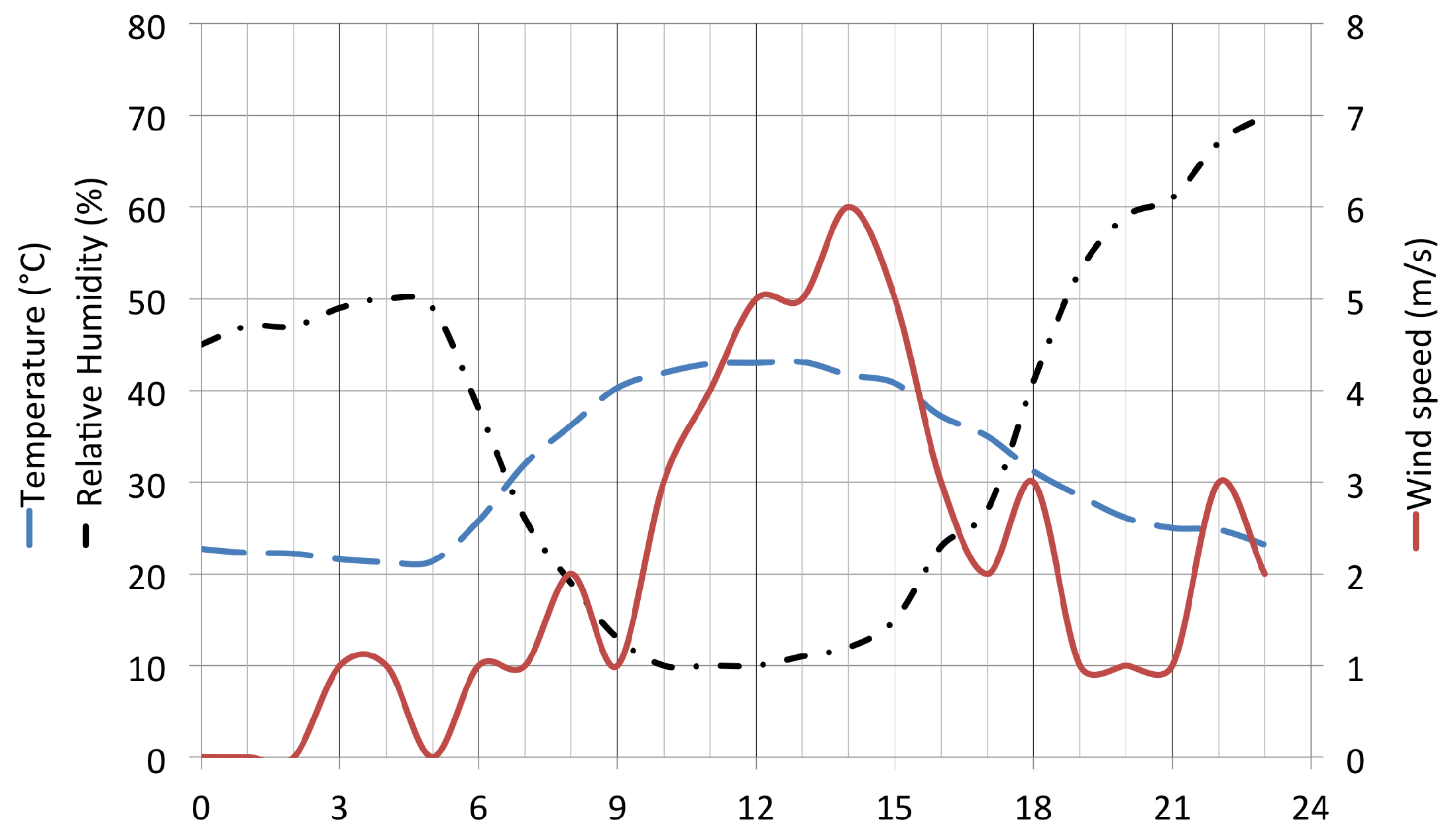
Figure 1 shows the diurnal variation of temperature, relative humidity and wind speed measured at the Sartene weather station located 20 km away from the fire. The hours prior to the fire were characterized by extreme weather conditions with low relative humidity (10%), very high temperatures (more than 40 C) and low to moderate winds (up to 6 ).
The landscape of the region is typical of the Corsican mountains with a 8 km-wide and 30 km-long valley starting at sea level with elevation rising to more than 2000 m. The fire started at 13:26 UTC and was very active during the first 6 h. Fire fighting actions and an increase in relative humidity slowed down the fire progression at around 19:00 UTC, stopping the propagation at sunset (21:00 UTC). Containment actions handled during the first hour were mainly unsuccessful. Then, during the most active propagation time, all the fire fighting actions were concentrated on the north flanks to prevent the fire from expanding to the next valley.
3.2. Numerical Configuration
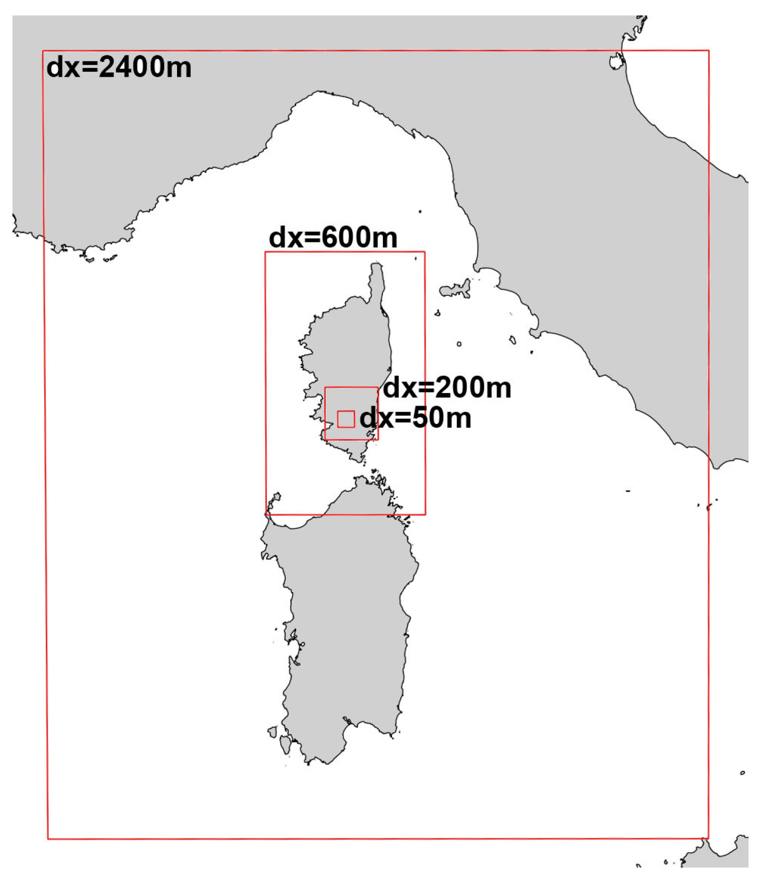
In order to resolve the development of the fire/weather system from the fire front to the large-scale atmospheric transport of the fire plume, the two-way nesting capability of the Meso-NH model is applied with four nested domains (Figure 2). The horizontal grid size is 2400 m for the outer domain covering 600 km × 720 km. The inner computational grids have grid increments of respectively 600, 200 and 50 m, covering a total area of respectively 144 km × 240 km, 48 km × 48 km and 15 km × 15 km for the innermost model. The time step is 12 s for the outermost model and decreases to 6 s, 2 s and 0.5 s for the finer models.
Initial and lateral boundary conditions are provided by the Aladin limited-area model (10-km horizontal resolution) operational at Meteo-France in 2009, with updates of the coupling files every 6 h. The simulation with the coarsest resolution began on 23 July 2009 at 0000 UTC, with a progressive downscaling up to the finest resolution beginning at 1200 UTC.
The vertical resolution is identical for all the nested domains, with 66 levels up to 10 km and a first level above the ground at 10-m height. All the nested models use the one and a half order closure turbulence scheme of [39] with a prognostic TKE: the three finest resolution domains use the 3D version of the scheme, while the first one only considers the 1D version, neglecting the horizontal turbulent fluxes. In addition, the 200-m and 50-m resolution domains consider the [40] mixing length, while the first two use the one of [41]. In the same way, only the coarsest model uses the [42] mass flux scheme to parametrize the thermals in the atmospheric boundary layer while they are explicitly resolved at a finer scale.
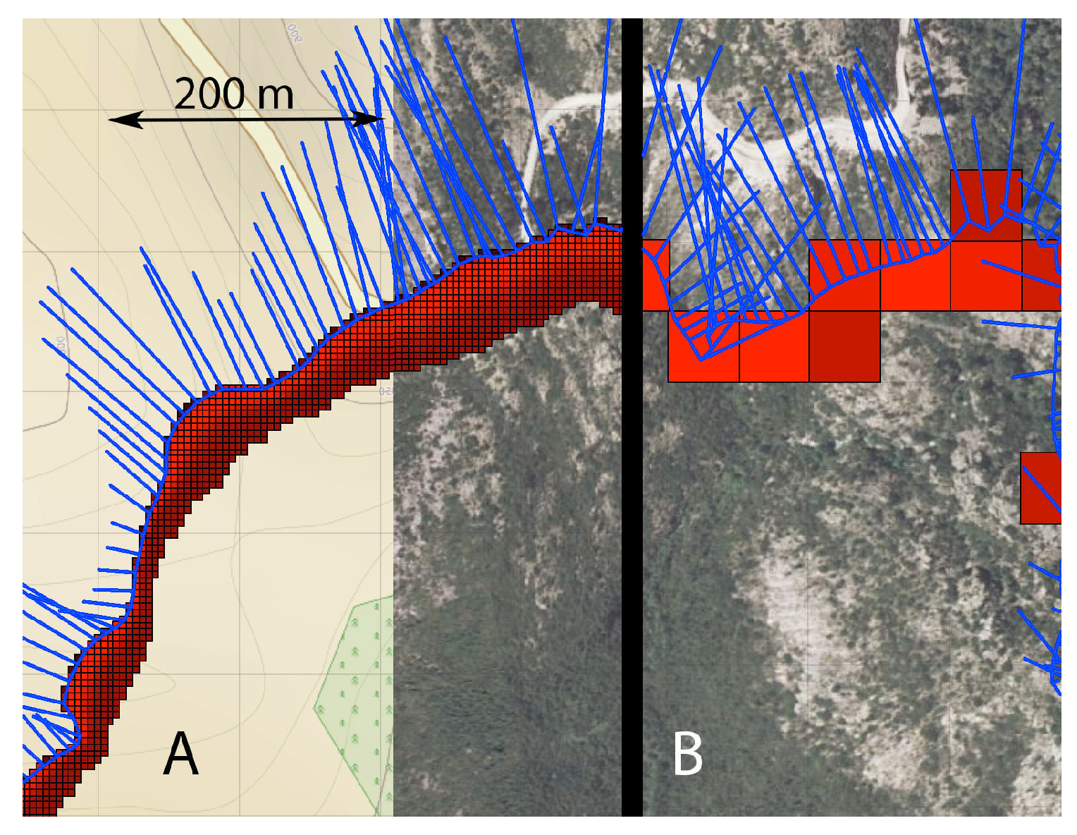
The fire propagation resolution is m, with perimeter and AT matrix resolution m. Fire resolutions are illustrated in Figure 3, which presents the successive scales from the front (markers) to combustion (arrival time matrix), integrated at the horizontal atmospheric resolution to provide fire fluxes forcing to Meso-NH. The resolution m of the fire propagation model is limited by the actual resolution of the fuel distribution data.
Three different simulations have been run to conduct a sensitivity study of the coupling method. The main simulation is the “coupled” coupling simulation, or “feedback-on”, where the interaction between the atmospheric and fire models is two-way, as described above. An “uncoupled” simulation was run, or “feedback-off”, where the atmospheric winds are provided to the fire model, but the fire model returns nothing to the atmosphere. The third simulation is the “fire-to-atm ” mode where Meso-NH wind fields are not used by ForeFire, so there is no fire-line propagation with the marker method. A pre-computed arrival time matrix is used to compute the fluxes at each atmospheric time step. This matrix is computed using a simulation of the fire with the integration of the modified fuel distribution to represent fire-fighting actions (massive air attack at the flanks and at the fire head around the end of the fire). The “feedback-off” wind field at 14 UTC was selected for this fire-to-atm arrival time matrix as it provided the best fit to match observed fire passing points and final shape. In return, ForeFire provides the modified surface fluxes to Meso-NH. “Feedback-off” simulations can be used if the forecast starts from an already developed fire (with an actual observed burning area), or to investigate a “what-if” scenario of a fire simulated without the overhead of the atmospheric model.
3.3. Data Sources
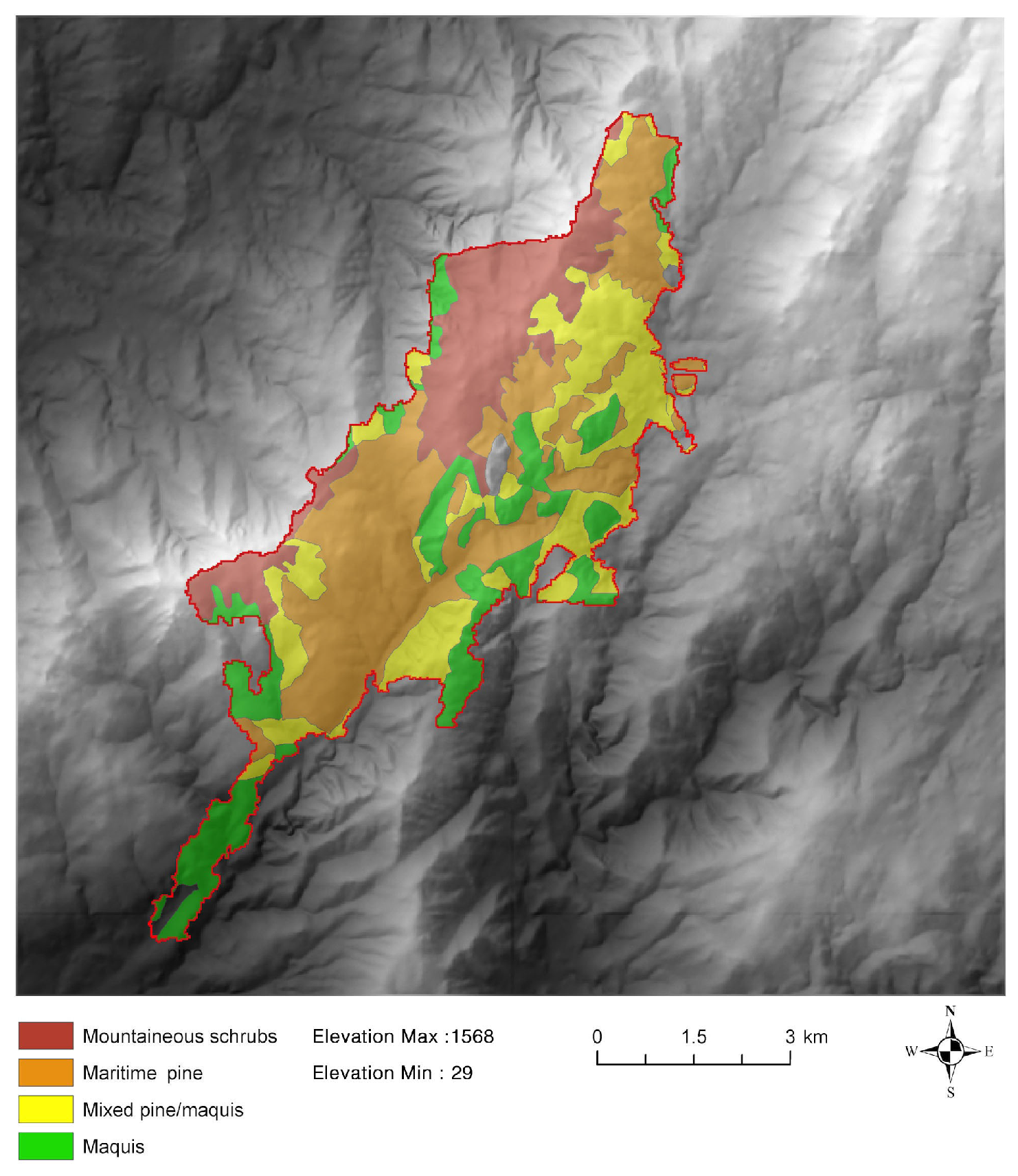
The fuel layer is derived from the National Forest Inventory and is coupled with data from the IGN BD TOPO® for road and drainage networks. The Digital Elevation Model (DEM) is extracted from IGN BD ALTI® 25-m resolution. IFN classes have been grouped according to the methodology developed in [43] and use the proposed characterization of the vegetation. Figure 4 presents the fuel distribution over the final burnt area, with four main classes, as well as small non-burnable area providing fuel breaks. Vegetation heterogeneity, orography or small unreported older fires influence the fire propagation at small scales. These heterogeneities are not accounted for in this work, and the chosen fuel types are taken as the best guesses.
Fuel parameters (mass loading , height E (m), moisture content (m) and heat of combustion ) used in the front velocity model for these four major classes are presented in Table 1. These values correspond to the dead fuel load of relatively small particles (branches with diameters less than m) that are assumed to drive the flaming fire. Pine and mixed pines’ fuel estimates are equivalent fuel types that were given by foresters in charge of the area. Except from the maquis, where estimates of similar species are available from [43], it was not possible to match with the foresters any relevant fuel characterization available in the literature. Moisture content was estimated to be very dry with values for the day reported well under 10% for shrubs. The same parameters were used for the fluxes’ models, with only the thin fuel contributing to heat injection, focusing the intense effects on the active fire area. Although the omission of larger fuel particle probably under-evaluates the contribution of the fire, it is consistent with the assumptions of the velocity model.
4. Simulation Results
4.1. Qualitative Results of the “Coupled” Simulation
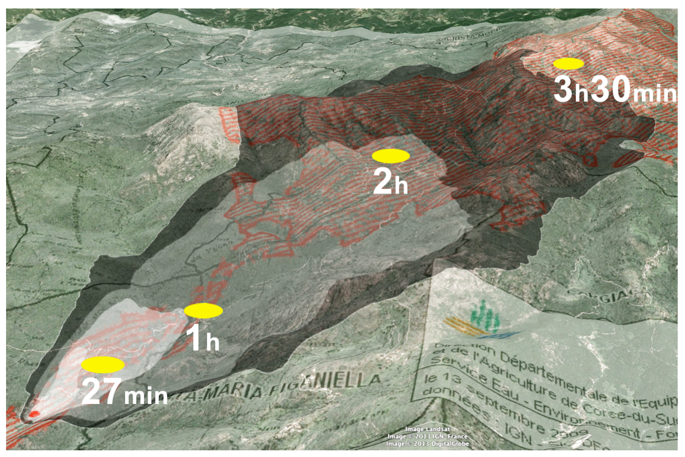
In this part, we qualitatively describe the results of the “coupled” simulation. The simulated fire behavior is difficult to assess, as fire fighters were very active (except during the first hour), influencing strongly the fire propagation (and thus the local circulation), but clear reports of fire fighting actions do not exist. The only information of the fire dynamics comes from reports of fire front passage, as shown in Figure 5. Without taking into account fire fighting actions, the “coupled” simulation obviously overestimates the global area burnt, except during the first hour, where the limited fighting actions were almost inefficient.
However, generally, the simulated front positions appear to approximate correctly the reported location of the fire head that could not be contained.
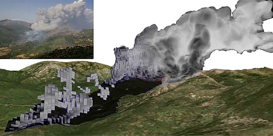
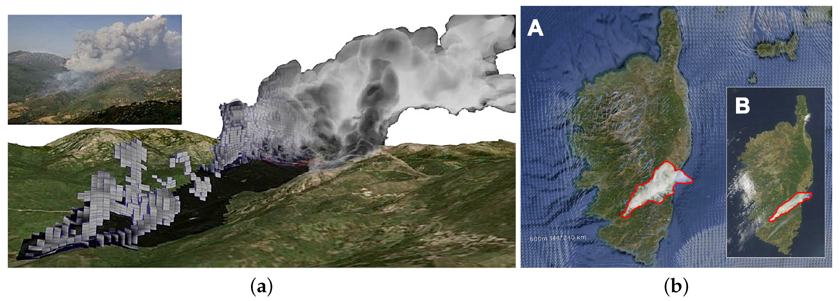
The simulated fire plume shows a good degree of realism at the local scale at 50-m resolution (Figure 6a). The simulated boundary layer, analyzed in the next section, reaches approximately 2200 m above ground level in reasonable agreement with a sounding from a nearby (30 km) Ajaccio airport launched 3 h before. Once injected in the free troposphere, the fire plume is advected and diluted by larger scale winds and turbulence. The fire plume simulated in the coarser model domain at 600-m resolution is advected northeastward, 40 km downwind of the fire ignition area (Figure 6b). This compares well with the plume direction and extension observed from MODIS.
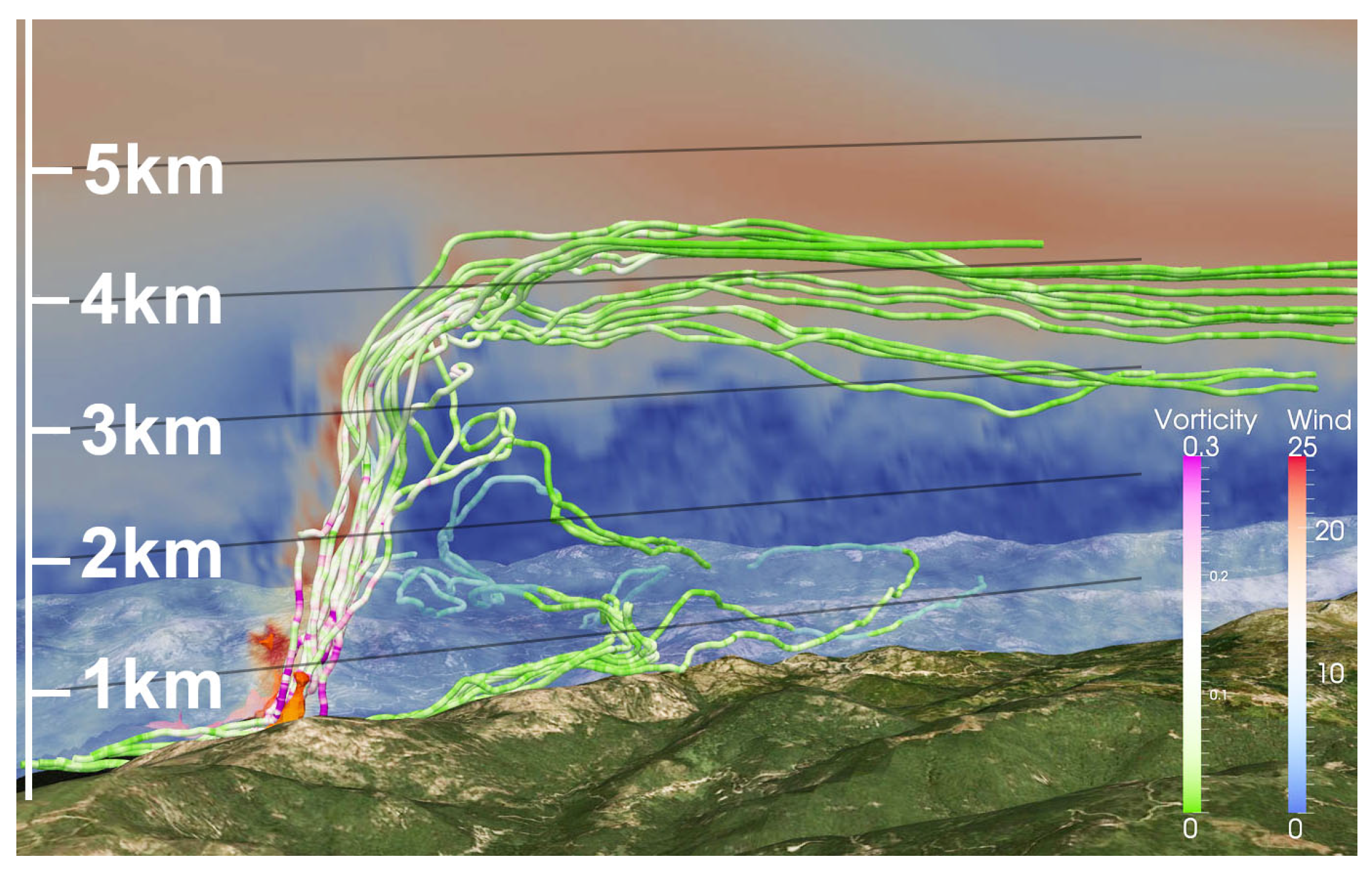
Figure 7 shows the wind acceleration near the surface and high wind speed values, which propagate along the fire-induced convective column reaching a 4500-m height. The colored streamlines reveal the vorticity magnitude in the ascending core of the fire plume. Fires are known to create vortices [44], and although it is out of scope for this study to characterize specific whirl structures at the fire front scale, fire-induced vorticity in the vicinity of the front can be resolved because of the high horizontal resolution. An animated visualization of the simulation is available as video supplementary material.
We can conclude that the “coupled” simulation shows a plausible development of the fire propagation according to available observations and can be further studied.
4.2. Dynamical Plume Structure
One of the aims of the current study is to use numerical simulations to better understand fire and atmosphere interactions. Figure 8 presents the fire front of the “uncoupled” and “coupled” simulations at 1500 UTC with the near-surface winds. The simulated fire spreads more rapidly on the north flanks of the valley, inducing convergent winds. The difference between the “coupled” and “uncoupled” simulations is analyzed to quantify the impact of the fire on the atmosphere. Perturbed surface winds occur around 3 km around the fire front (Figure 8c). Fire-induced surface winds reach more than five-times the background ambient winds throughout the fire with horizontal motion differences up to 20 . The fire not only modifies the dynamics near the surface, but creates a plume of almost 5000 m in depth (Figure 9). Instantaneous upward vertical velocities in the plume reach values of 27 , with pockets of peak values being produced above the boundary layer. Comparing simulated magnitudes to the observation of other instrumented wildfires is a little bit hazardous, as we cannot expect the values to be the same for all fires. It just allows one to control the order of magnitude of the simulated values. Only few large-scale experiments [45,46] were conducted and mainly on crown fires. In this respect, simulated updrafts appear in agreement with [45], who observed updraft values on the order of 20–30 , and [46], who reported peaks of 32–60 for crown fires occurring at the highest detectable heights (about 50 m). The largest simulated downward motion occurs in the upper plume behind the fire front (maximum of −7 ), consistent with previous observations [47] and simulations [48].
Differences in sensible heat flux at a 20-m height show maximum values of 240 (Figure 10d), which fall within the range of sensible heat fluxes as reported by [49]. They induce maxima of the 2-m temperature difference over the active fire area up to 70 K (Figure 10c). This generates a near-surface convergence zone in the active fire area (negative values of Figure 11a) and areas of near-surface divergence consecutive to downdrafts directly behind the fire front (Figure 8d) as a result of the pressure gradient caused by the convective plume and the air being drawn into the column (Figure 11b). The work in [48] suggested that downdrafts bring higher momentum near the surface and contribute to an increase in the rate of spread.
In the “uncoupled” simulation, a significant shear is present, with values of the order of 0.012 between a 1600-m and a 2600-m height (Figure 9a). The fire destroys the wind vertical gradient by inducing resolved eddies, with pockets of winds similar to the multi-cell distribution of convective cores described by [50] (Figure 9b). Unresolved eddies at 50-m resolution are also developed in the fire plume, with strong TKE values exceeding 20 , almost ten-times the background values of the planetary boundary layer (Figure 12a,b). The two main contributions of the TKE production are presented in Figure 12c,d. Near the surface, the thermal production is higher than the shear contribution due to a large increase in the sensible heat flux. However, above in the plume, the dynamics mainly controls the TKE production, probably partly due to the initial shear environment and partly due to the shear induced by the updraft itself.
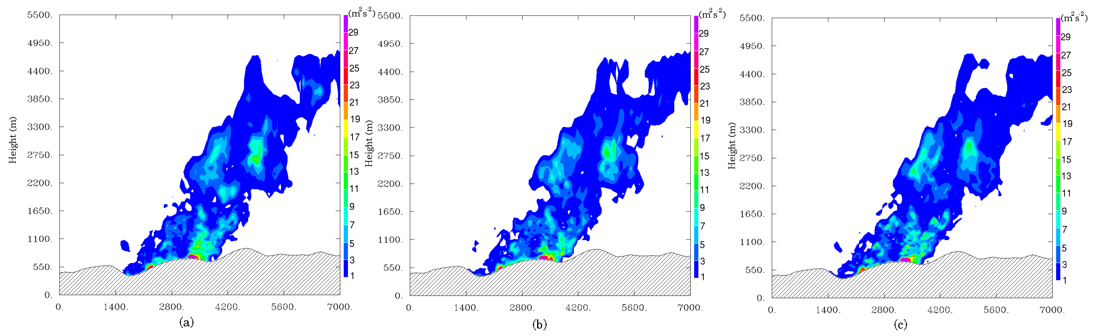
In agreement with observational studies [47,49], the simulation shows increases in both horizontal and vertical velocity variances at the fire front and above, up to a 5000-m height (Figure 13). Simulated values are in the same order of magnitude as the LiDAR observation of [49] reporting maximum variance values from 7 to 14 in a plume overshooting with comparable height. The simulated turbulence associated with the fire front is characterized by quasi-isotropic behavior with both high horizontal and vertical variances associated with fire-induced winds at the fire-front (Figure 14). The spectral analysis reveals a general increase in the vertical velocity spectral energy at all wavelengths with the fire-atmosphere coupling, velocity spectra obeying the −5/3 slope in the inertial subrange well.
When taking into account fire fighting actions in the “fire-to-atm” simulation, the fire is less active on its lateral flanks and progresses more quickly toward the northeast (Figure 15), inducing an advance of about 1 km at 1500 UTC. The structure and the magnitude of dynamical fields are similar with strong fire-induced surface winds producing a convergence zone ahead of the surface and a convective column reaching the same height with strong updrafts and unresolved eddies mainly produced by shear. This underlines the systematic structure induced by the fire-atmosphere interactions in this configuration of the Aullene fire.
4.3. Computational Time
Computations were performed on the computer Jade at CINES (Centre Informatique National de l’Enseignement Supérieur) on 900 processors (Intel XEON types). Fire simulation overhead was estimated between 10 and 15% in the “coupled” and “fire-to-atm” cases compared to the “uncoupled” one, as can be seen in Table 2.
Faster than real-time (and operational) simulations have already been performed successfully by both CAWFE [51] and WRF/SFire [16] on larger fires, but the major asset of our simulation is mainly a higher resolution mesh (50 m compared to 200 m or more) applied to an extreme fire case. This goal was reached here by running in depopulated mode (using only two cores per compute node instead of eight), still on 900 processors (but with 3600 mobilized) on Jade, as it increases the memory bandwidth available per node. In this case, it was possible to obtain a 0.76 calculation ratio, below real time. Although this ratio is too large to consider operational uses (a forecast framework will impose a computation speed at least twice as fast), it is important to note that a factor between two and four in computation time is expected in the newer version of Meso-NH: the factor of four would correspond to the use of the Weighted Essentially Non-Oscillatory (WENO) scheme for momentum transport, but with a coarser effective resolution due to its diffusive character, while the factor of two would be brought by the WENO of fifth order [52], or the fourth order centered scheme associated with a fourth order Runge–Kutta time-splitting marching instead of the LF scheme [21]. This constitutes an interesting prospect for operational wildfire prediction. The fire-to-atm cases are here the most expensive cases mainly because this makes intensive and non-optimized use of the file system to read the fire progression file.
5. Conclusions
The coupled code Meso NH/ForeFire aims to be able to simulate large wildfires, solving complex fire-induced flow while implementing a high-resolution front advection method. The fire front velocity model can be parametrized with measurable properties of the fuel and is well adapted to coupled simulation, as it uses instantaneous wind speed just over the fire front to calculate the flame angle. The non-parallel version of the code has previously been used to perform simulations of real wildfires with results that qualitatively match observation in terms of fire dynamics [9] and atmospheric chemistry [53].
The embedded parallel strategy demonstrated in this study ensures that the coupled model will behave in the same way as the atmospheric model and thus will benefit from further improvements. The system proves to be able to simulate a large wildfire, although with some arguable simplifications of important processes and relatively raw parametrization given the complex landscape. It makes it possible to simulate both the fine-scale fire-atmosphere interactions occurring at tens of meters scales around the fire front and larger regional scales with a good degree of realism. The multiscale simulation allowed exploring the dynamical structure of the surrounding atmosphere. Wildland fire induced strong surface winds generating a few thousand meter convective column with pockets of updrafts, stronger at higher levels and following a multi-cell distribution, while strong downdrafts occurred behind the plume and the fire front. At 50-m resolution, subgrid motions as well as the resolved momentum were strongly enhanced by the fire. Shear had a larger contribution than buoyancy to the turbulence within the fire plume partly due to high sheared initial winds.
It is reasonable to think that such coupled models will run faster than real time on medium-sized clusters in the near future. This type of coupled simulation could then become a decision support tool, forecasting plume size, transport dispersion and smoke concentration at the ground (information of prime importance to protect the population) and anticipating the visibility loss for the fire fighters and civil transport in general. In terms of forecasting the fire-line location, it is unlikely that such models ever reach the ability and precision of very fast codes that can be tweaked and adapted in real time to fire observations and fighting scenarios. Nevertheless, such codes still require wind, temperature and more generally changing weather pattern forecasts. Fire to atmosphere numerical coupling appears to be a reasonable way of forecasting extreme weather events that can strongly affect local meteorological conditions.
The major point was to demonstrate and build the platform that may now receive enhancement from the community, as all codes are open source.
The main plan is to improve fuel models, as well as the fire velocity and surface flux models in order to better represent the combustion phase that will refine the diagnosis of turbulent fluxes at the ground level and the combustion phase of larger fuel particles. The simulation of more systematic very large wildfires at high resolution with a complex fuel structure is the current goal for model validation, along with the development of an operational tool chain for fire and fire-weather forecasting if sufficient performance can be achieved.
Supplementary Materials
The following are available online at https://www.mdpi.com/2073-4433/9/6/218/s1.
Author Contributions
J.-B.F. redacted the main text, designed and implemented the coupled fire code, the experiment and performed the simulations and post-processing. F.B. prepared the fuel data, figure and performed some preliminary simulations. C.M. designed the surface injection model and performed the analysis of the plume. C.L. is the lead developer of the atmospheric model, designed the atmospheric grids and parameterization and provided the analysis and figures of the fire-atmosphere interactions.
Acknowledgments
This research is supported by the Agence Nationale de la Recherche, Project ANR-09-COSI- 006, ANR-16-CE04-0006 and the CINES Computing center Jade computer under grant DARIc20132b1723.
Conflicts of Interest
The authors declare no conflict of interest.
References
- Sun, R.; Krueger, S.K.; Jenkins, M.A.; Zulauf, M.A.; Charney, J.J. The importance of fire–atmosphere coupling and boundary-layer turbulence to wildfire spread. Int. J. Wildland Fire 2009, 18, 50–60. [Google Scholar] [CrossRef]
- Linn, R.; Reisner, J.; Colman, J.; Winterkamp, J. Studying wildfire behavior using FIRETEC. Int. J. Wildland Fire 2002, 11, 233–246. [Google Scholar] [CrossRef] [Green Version]
- Mell, W.; Jenkins, M.; Gould, J.; Cheney, P. A physics-based approach to modelling grassland fires. Int. J. Wildland Fire 2007, 16, 1–22. [Google Scholar] [CrossRef]
- Morvan, D. Modeling of fire spread through a forest fuel bed using a multiphase formulation. Combust. Flame 2001, 127, 1981–1994. [Google Scholar] [CrossRef]
- Morvan, D. Modeling the propagation of a wildfire through a Mediterranean shrub using a multiphase formulation. Combust. Flame 2004, 138, 199–210. [Google Scholar] [CrossRef]
- Finney, M. FARSITE: Fire Area Simulator–Model Development and Evaluation—Research Paper RMRS-RP-4 Revised; Technical Report; U.S. Department of Agriculture, Forest Service, Rocky Mountain Research Station: Ogden, UT, USA, 2004. [Google Scholar]
- Clark, T.; Jenkins, M.; Coen, J.; Packham, D. A Coupled Atmosphere Fire Model: Convective Feedback on Fire-Line Dynamics. J. Appl. Meteorol. 1996, 35, 875–901. [Google Scholar] [CrossRef]
- Mandel, J.; Beezley, J.; Kochanski, A. Coupled atmosphere-wildland fire modeling with WRF 3.3 and SFIRE 2011. Geosci. Model Dev. 2011, 4, 591–610. [Google Scholar] [CrossRef] [Green Version]
- Filippi, J.; Bosseur, F.; Pialat, X.; Santoni, P.; Strada, S.; Mari, C. Simulation of Coupled Fire/Atmosphere Interaction with the MesoNH-ForeFire Models. J. Combust. 2011, 2011, 1–13. [Google Scholar] [CrossRef] [Green Version]
- Heilman, W.; Fast, J. Simulations of Horizontal Roll Vortex Development Above Lines of Extreme Surface Heating. Int. J. Wildland Fire 1992, 2, 55–68. [Google Scholar] [CrossRef]
- Clark, T.; Jenkins, M.; Coen, J.; Packham, D. A Coupled Atmosphere-Fire Model: Role of the Convective Froude Number and Dynamic Fingering at the Fireline. Int. J. Wildland Fire 1996, 6, 177–190. [Google Scholar] [CrossRef] [Green Version]
- Rothermel, R. A Mahematical Model for Predicting Fire Spread in Wildland Fuels; Technical Report; USDA Forest Service: Washington, DC, USA, 1972. [Google Scholar]
- Clark, T.; Coen, J.; Latham, D. Description of a coupled atmosphere-fire model. Int. J. Wildland Fire 2004, 13, 49–63. [Google Scholar] [CrossRef]
- Coen, J. Modeling Wildland Fires: A Description of the Coupled Atmosphere-Wildland Fire Environment Model (CAWFE); Technical Report; UCAR/NCAR: Boulder, CO, USA, 2013. [Google Scholar]
- Skamarock, W.; Klemp, J. A time-split nonhydrostatic atmospheric model for weather research and forecasting applications. J. Comput. Phys. 2008, 227, 3465–3485. [Google Scholar] [CrossRef]
- Kochanski, A.; Jenkins, M.; Mandel, J.; Beezley, J.; Krueger, S. Real time simulation of 2007 Santa Ana fires. For. Ecol. Manag. 2013, 294, 136–149. [Google Scholar] [CrossRef]
- Coen, J.L.; Cameron, M.; Michalakes, J.; Patton, E.G.; Riggan, P.J.; Yedinak, K.M. WRF-Fire: Coupled Weather–Wildland Fire Modeling with the Weather Research and Forecasting Model. J. Appl. Meteorol. Climatol. 2013, 52, 16–38. [Google Scholar] [CrossRef] [Green Version]
- Peace, M.; Mattner, T.; Mills, G.; Kepert, J.; McCaw, L. Coupled Fire–Atmosphere Simulations of the Rocky River Fire Using WRF-SFIRE. J. Appl. Meteorol. Climatol. 2016, 55, 1151–1168. [Google Scholar] [CrossRef]
- Coen, J. Simulation of the Big Elk Fire using coupled atmosphere-fire modeling. Int. J. Wildland Fire 2005, 14, 49–59. [Google Scholar] [CrossRef]
- Lafore, J.; Stein, J.; Asencio, N.; Bougeault, P.; Ducrocq, V.; Duron, J.; Fischer, C.; Héreil, P.; Mascart, P.; Masson, V.; et al. The Meso-NH Atmospheric Simulation System. Part I: adiabatic formulation and control simulations. Ann. Geophys. 1998, 16, 90–109. [Google Scholar] [CrossRef] [Green Version]
- Lac, C.; Chaboureau, J.P.; Masson, V.; Pinty, J.P.; Tulet, P.; Escobar, J.; Leriche, M.; Barthe, C.; Aouizerats, B.; Augros, C.; et al. Overview of the Meso-NH model version 5.4 and its applications. Geosci. Model Dev. 2018, 11, 1929–1969. [Google Scholar] [CrossRef]
- Balbi, J.; Morandini, F.; Silvani, X.; Filippi, J.; Rinieri, F. A Physical Model for Wildland Fires. Combust. Flame 2009, 156, 2217–2230. [Google Scholar] [CrossRef]
- Rothermel, R. How to Predict the Spread and Intensity of Forest and Range Fire, Tech. Rep. INT-143; Technical Report; USDA Forest Research Service: Washington, DC, USA, 1983. [Google Scholar]
- Filippi, J.; Morandini, F.; Balbi, J.; Hill, D. Discrete Event Front-tracking Simulation of a Physical Fire-spread Model. Simulation 2009, 86, 629–646. [Google Scholar] [CrossRef] [Green Version]
- Filippi, J.; Bosseur, F.; Mari, C.; Lac, C.; Moigne, P.L.; Cuenot, B.; Veynante, D.; Cariolle, D.; Balbi, J. Coupled atmosphere-wildland fire modelling. J. Adv. Model. Earth Syst. 2009, 1. [Google Scholar] [CrossRef]
- Filippi, J.; Pialat, X.; Clements, C. Assessment of ForeFire/Meso-NH for wildland fire/atmosphere coupled simulation of the FireFlux experiment. Proc. Combust. Inst. 2013, 34, 2633–2640. [Google Scholar] [CrossRef]
- Colella, P.; Woodward, P. The Piecewise Parabolic Method (PPM) for gas-dynamical simulations. J. Comput. Phys. 1984, 54, 174–201. [Google Scholar] [CrossRef] [Green Version]
- Ricard, D.; Lac, C.; Riette, S.; Legrand, R.; Mary, A. Kinetic energy spectra characteristics of two convection- permitting limited-area models AROME and Meso-NH. Q. J. R. Meteorol. Soc. 2012, 139, 1327–1341. [Google Scholar] [CrossRef]
- Masson, V.; Moigne, P.L.; Martin, E.; Faroux, S.; Alias, A.; Alkama, R.; Belamari, S.; Barbu, A.; Boone, A.; Bouyssel, F.; et al. The SURFEXv7.2 land and ocean surface platform for coupled or offline simulation of earth surface variables and fluxes. Geosci. Model Dev. 2013, 6, 929–960. [Google Scholar] [CrossRef] [Green Version]
- Noilhan, J.; Planton, S. A simple parameterization of land surface processes for meteorological models. Monthly Weather Rev. 1989, 117, 536–549. [Google Scholar] [CrossRef]
- Maitre, E. Review of numerical methods for free interfaces. Ecole Thématique “Modèles de champ de phase pour l’évolution de structures complexes”. Les Houches 2006, 27, 31. [Google Scholar]
- Tryggvason, G.; Bunner, B.; Esmaeeli, A.; Juric, D.; Al-Rawahi, N.; Tauber, W.; Han, J.; Nas, S.; Jan, Y. A Front-Tracking Method for the Computations of Multiphase Flow. J. Comput. Phys. 2001, 169, 708–759. [Google Scholar] [CrossRef] [Green Version]
- Harlow, F.; Welch, J. Numerical calculation of time-dependent viscous incompressible flow of fluid with free surface. Phys. Fluids 1965, 8, 2182–2189. [Google Scholar] [CrossRef]
- Filippi, J.; Mallet, V.; Nader, B. Evaluation of forest fire models on a large observation database. Nat. Hazards Earth Syst. Sci. 2014, 14, 3077–3091. [Google Scholar] [CrossRef] [Green Version]
- Karimabadi, H.; Driscoll, J.; Omelchenko, Y.; Omidi, N. A new asynchronous methodology for modeling of physical systems: breaking the curse of courant condition. J. Comput. Phys. 2005, 205, 755–775. [Google Scholar] [CrossRef] [Green Version]
- Albini, F.; Brown, J.; Reinhardt, E.; Ottmar, R. Calibration of a Large Fuel Burnout Model. Int. J. Wildland Fire 1995, 5, 173–192. [Google Scholar] [CrossRef]
- Morvan, D. Numerical study of the effect of fuel moisture content (FMC) upon the propagation of a surface fire on a flat terrain. Fire Saf. J. 2013, 58, 121–131. [Google Scholar] [CrossRef]
- Anderson, H. Heat Transfer and Fire Spread; USDA Forest Service Research Paper INT, Intermountain Forest and Range Experiment Station, Forest Service; U.S. Department of Agriculture: Washington, DC, USA, 1969.
- Cuxart, J.; Bougeault, P.; Redelsperger, J.L. A turbulence scheme allowing for mesoscale and large-eddy simulations. Q. J. R. Meteorol. Soc. 2000, 126, 1–30. [Google Scholar] [CrossRef]
- Deardorff, J.W. Stratocumulus-capped mixed layers derived from a three-dimensional model. Bound.-Lay. Meteorol. 1980, 18, 495–527. [Google Scholar] [CrossRef]
- Bougeault, P.; Lacarrere, P. Parameterization of Orography-Induced Turbulence in a Mesobeta–Scale Model. Mon. Weather Rev. 1989, 117, 1872–1890. [Google Scholar] [CrossRef]
- Pergaud, J.; Masson, V.; Malardel, S.; Couvreux, F. A Parameterization of Dry Thermals and Shallow Cumuli for Mesoscale Numerical Weather Prediction. Bound.-Lay. Meteorol. 2009, 132, 83–106. [Google Scholar] [CrossRef]
- Santoni, P.; Filippi, J.; Balbi, J.; Bosseur, F. Wildland Fire Behaviour Case Studies and Fuel Models for Landscape-Scale Fire Modeling. J. Combust. 2011, 2011, 613424. [Google Scholar] [CrossRef]
- Forthofer, J.; Goodrick, S. Review of Vortices in Wildland Fire. J. Combust. 2011, 2011, 984363. [Google Scholar] [CrossRef]
- Clark, T.L.; Radke, L.; Coen, J.; Middleton, D. Analysis of Small-Scale Convective Dynamics in a Crown Fire Using Infrared Video Camera Imagery. J. App. Meteorol. 1999, 38, 1401–1420. [Google Scholar] [CrossRef] [Green Version]
- Coen, J.; Mahalingam, S.; Daily, J. Infrared Imagery of Crown-Fire Dynamics during FROSTFIRE. J. Appl. Meteor. 2004, 43, 1241–1259. [Google Scholar] [CrossRef] [Green Version]
- Clements, C.; Shiyuan, Z.; Xindi, B.; Warren, E.; Daewon, W. First observations of turbulence generated by grass fires. J. Geophys. Res. 2008, 113. [Google Scholar] [CrossRef] [Green Version]
- Sun, R.; Jenkins, M.A.; Krueger, S.K.; Mell, W.; Charney, J.J. An evaluation of fire-plume properties simulated with the Fire Dynamics Simulator (FDS) and the Clark coupled wildfire model. Can. J. For. Res. 2006, 36, 2894–2908. [Google Scholar] [CrossRef]
- Lareau, N.P.; Clements, C.B. The Mean and Turbulent Properties of a Wildfire Convective Plume. J. Appl. Meteorol. Climatol. 2017, 56, 2289–2299. [Google Scholar] [CrossRef]
- Kiefer, M.T.; Parker, M.D.; Charney, J.J. Regimes of dry convection above wildfires: Idealized numerical simulations and dimensional analysis. J. Atmos. Sci. 2009, 66, 806–836. [Google Scholar] [CrossRef]
- Coen, J.; Schroeder, W. Use of spatially refined satellite remote sensing fire detection data to initialize and evaluate coupled weather-wildfire growth model simulations. Geophys. Res. Lett. 2013, 40, 5536–5541. [Google Scholar] [CrossRef] [Green Version]
- Lunet, T.; Lac, C.; Auguste, F.; Visentin, F.; Masson, V.; Escobar, J. Combination of WENO and Explicit Runge-Kutta methods for wind transport in Meso-NH model. Mon. Weather Rev. 2017, 145, 3817–3838. [Google Scholar] [CrossRef]
- Strada, S.; Mari, C.; Filippi, J.; Bosseur, F. Wildfire and the atmosphere: modelling the chemical and dynamic interactions at the regional scale. Atmos. Environ. 2012, 51, 234–249. [Google Scholar] [CrossRef]
Figure 1.
Sartene weather station records on 23 July 2009 (in hours UTC): temporal evolution of 10-m wind speed (in red, in ), 2-m temperature (in blue, in deg C) and relative humidity (in black, in %).
Figure 1.
Sartene weather station records on 23 July 2009 (in hours UTC): temporal evolution of 10-m wind speed (in red, in ), 2-m temperature (in blue, in deg C) and relative humidity (in black, in %).

Figure 2.
Overview of the nested Meso-NH domains.

Figure 3.
Aullene’s fire, markers (blue) and heat fluxes above 30 at fire resolution (5 m) (A) used to force the atmospheric surface fields (resolution 50 m) (B).
Figure 3.
Aullene’s fire, markers (blue) and heat fluxes above 30 at fire resolution (5 m) (A) used to force the atmospheric surface fields (resolution 50 m) (B).

Figure 4.
Overview of the fuel distributions with the four main fuel classes over the final observed fire area over elevation in gray shades.
Figure 4.
Overview of the fuel distributions with the four main fuel classes over the final observed fire area over elevation in gray shades.

Figure 5.
View of the “coupled” fire simulation (grey scale) 27 min, 1 h, 2 h and 3 h 30 after the beginning of the fire, with corresponding observed fire passing points (yellow marks), superimposed on the real burnt area including fire fighting actions (dashed red area). The horizontal extension at the base of the figure is 5 km.

Figure 6.
Simulated smoke tracer on 23 July 2009 (a) in the 50-m resolution domain compared to the plume’s photograph (at the top left) at 14:50 UTC and (b) in the 600-m resolution domain highlighted in red (A) at 15:00 UTC compared to the MODIS image (B) of Corsica at 14:50 UTC.
Figure 6.
Simulated smoke tracer on 23 July 2009 (a) in the 50-m resolution domain compared to the plume’s photograph (at the top left) at 14:50 UTC and (b) in the 600-m resolution domain highlighted in red (A) at 15:00 UTC compared to the MODIS image (B) of Corsica at 14:50 UTC.

Figure 7.
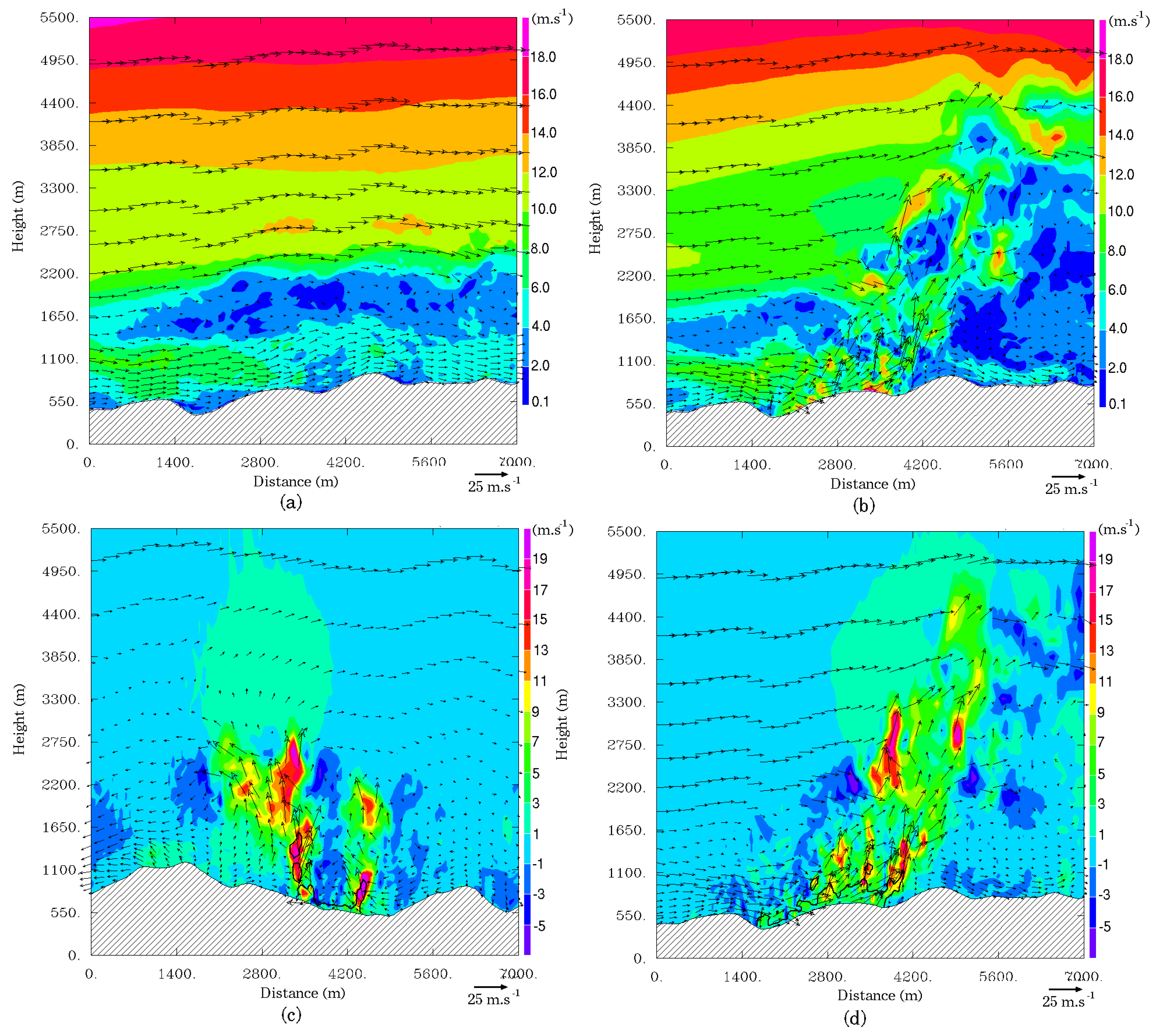
Vertical cross-section of the wind speed (in , between blue and red) and streamlines initiated at the ground and colored according to the vorticity (in , between green and pink) at 1500 UTC.
Figure 7.
Vertical cross-section of the wind speed (in , between blue and red) and streamlines initiated at the ground and colored according to the vorticity (in , between green and pink) at 1500 UTC.

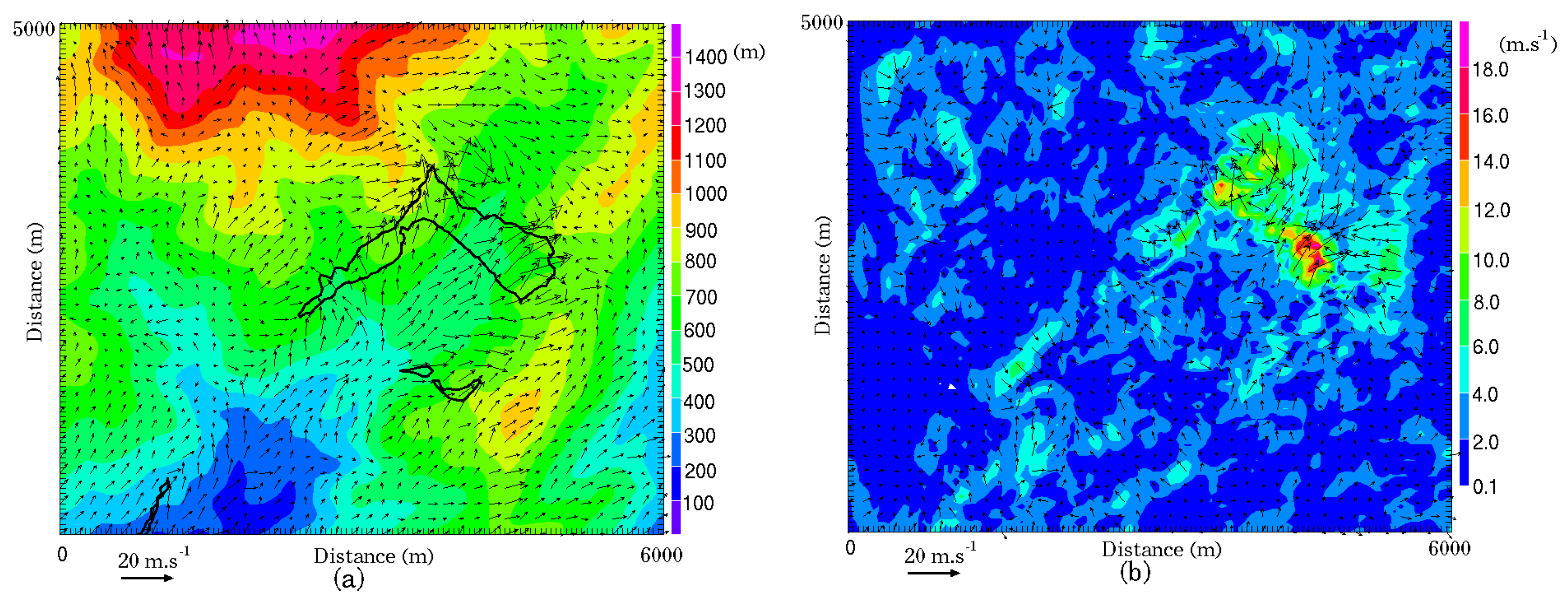
Figure 8.
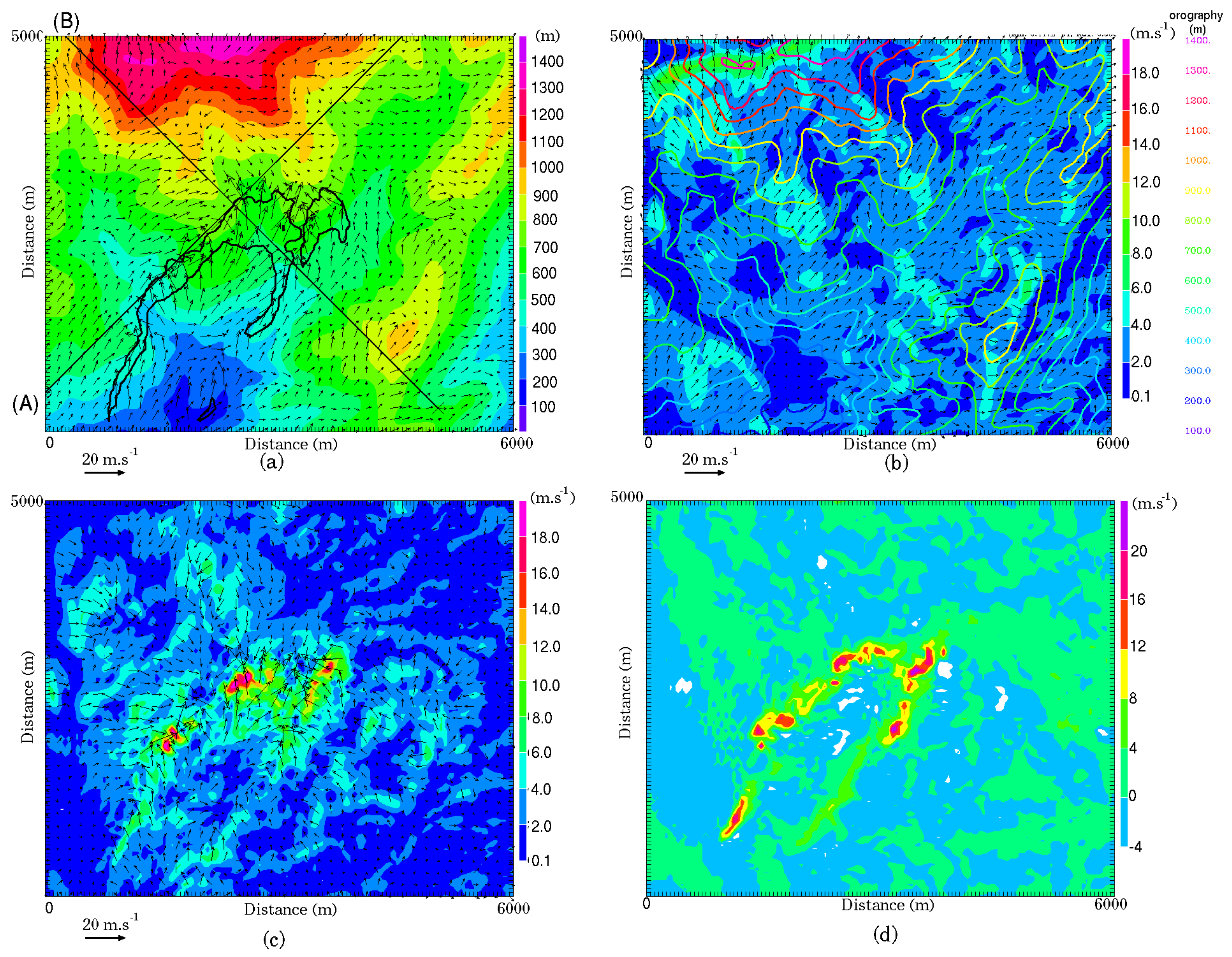
Horizontal cross-sections on 23 July 2009 at 1500 UTC: (a) envelop of the fire front (in black) at the ground superimposed on the 10-m wind vectors (arrows) of the “coupled” simulation and on the orography (color, in m) with the axis of the vertical cross-sections; (b,c) 10-m wind speed (in ) with wind vectors superimposed for the (b) “uncoupled” and (c) difference “coupled minus uncoupled” simulations; (d) Vertical velocity at a 300-m height (in ) for the difference “coupled minus uncoupled” simulations. Orography isocontours are superimposed in (b).
Figure 8.
Horizontal cross-sections on 23 July 2009 at 1500 UTC: (a) envelop of the fire front (in black) at the ground superimposed on the 10-m wind vectors (arrows) of the “coupled” simulation and on the orography (color, in m) with the axis of the vertical cross-sections; (b,c) 10-m wind speed (in ) with wind vectors superimposed for the (b) “uncoupled” and (c) difference “coupled minus uncoupled” simulations; (d) Vertical velocity at a 300-m height (in ) for the difference “coupled minus uncoupled” simulations. Orography isocontours are superimposed in (b).

Figure 9.
Vertical cross-sections on 23 July 2009 at 1500 UTC: (a,b) horizontal wind (in ) with wind vectors superimposed for (a) the “uncoupled” simulation and (b) the “coupled” one along the direction of propagation (axis (A) in Figure 8a); (c,d) vertical velocity difference between “coupled” and “uncoupled” simulations (in ) with the wind vectors (arrows) (c) across the fire front (axis (B)) and (d) along the direction of propagation (axis (A)).

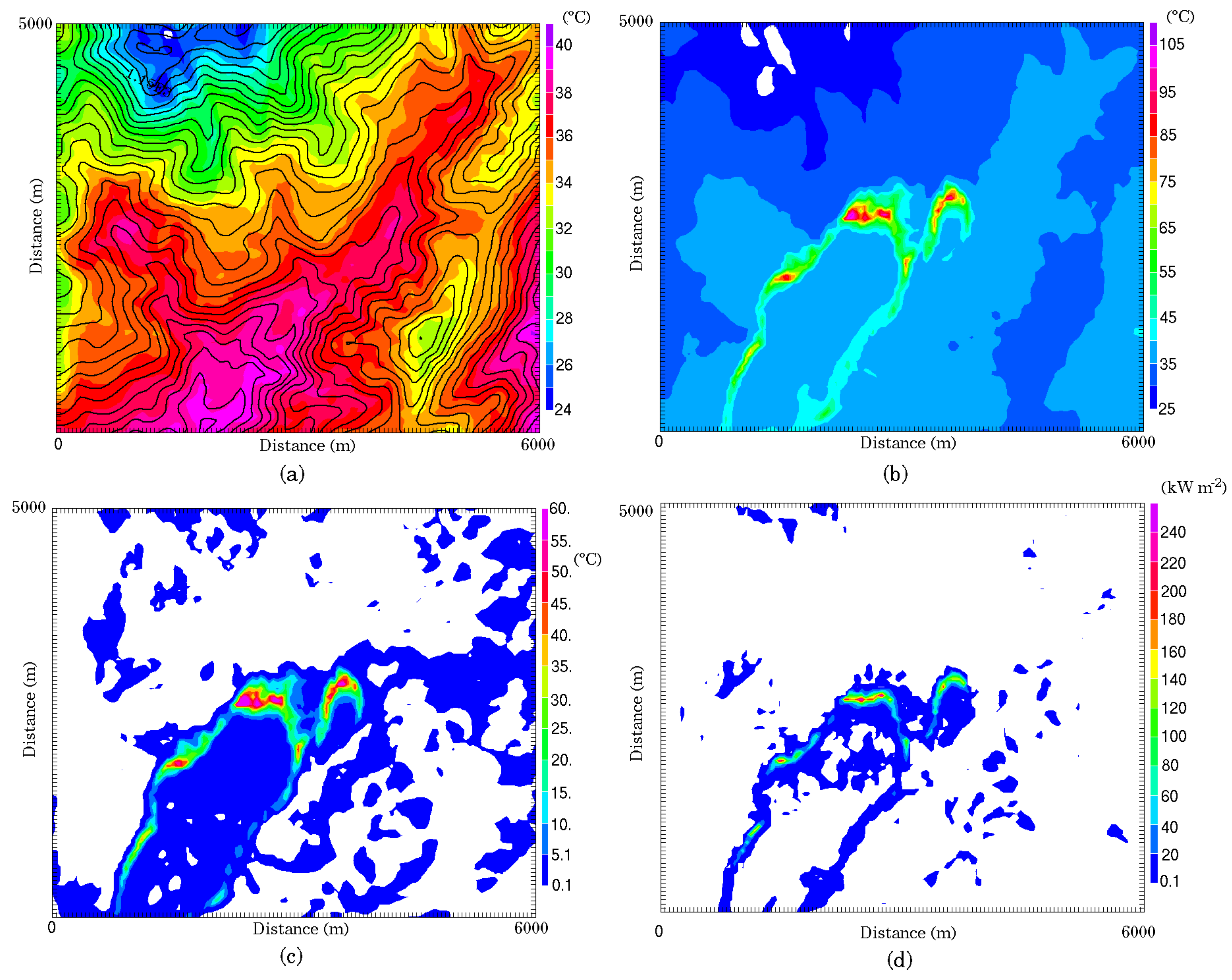
Figure 10.
Horizontal cross-sections on 23 July 2009 at 1500 UTC: 2-m temperature (in deg Celsius) for the (a) “uncoupled”; (b) “coupled” and (c) the difference “coupled minus uncoupled”; (d) Sensible heat flux at a 20-m height for the difference “coupled minus uncoupled” (in ). Isolines of orography are superimposed in (a).

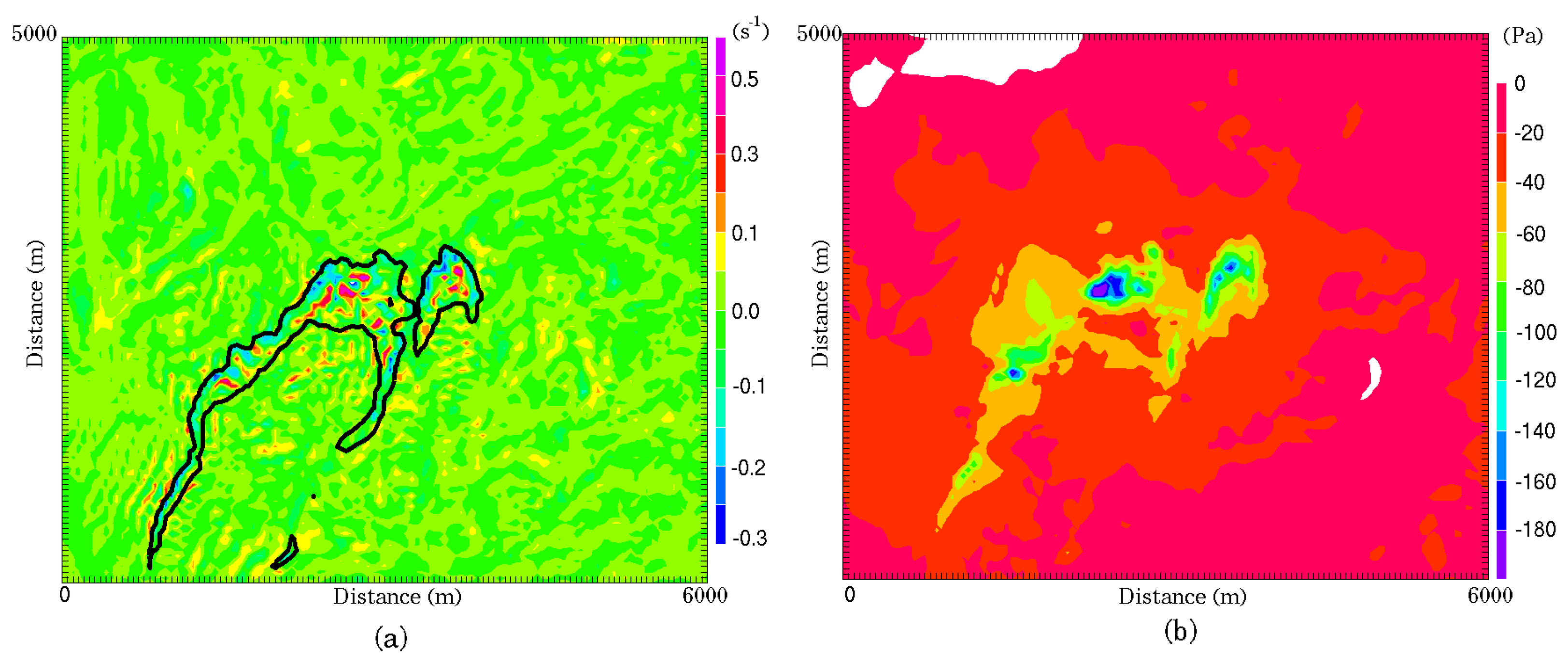
Figure 11.
Difference between “coupled” and “uncoupled” simulations on 23 July 2009 at 1500 UTC: Horizontal cross-sections of (a) 10-m horizontal divergence (in ) with the fire tracer superimposed (in black); (b) 10-m pressure (in Pa).
Figure 11.
Difference between “coupled” and “uncoupled” simulations on 23 July 2009 at 1500 UTC: Horizontal cross-sections of (a) 10-m horizontal divergence (in ) with the fire tracer superimposed (in black); (b) 10-m pressure (in Pa).

Figure 12.
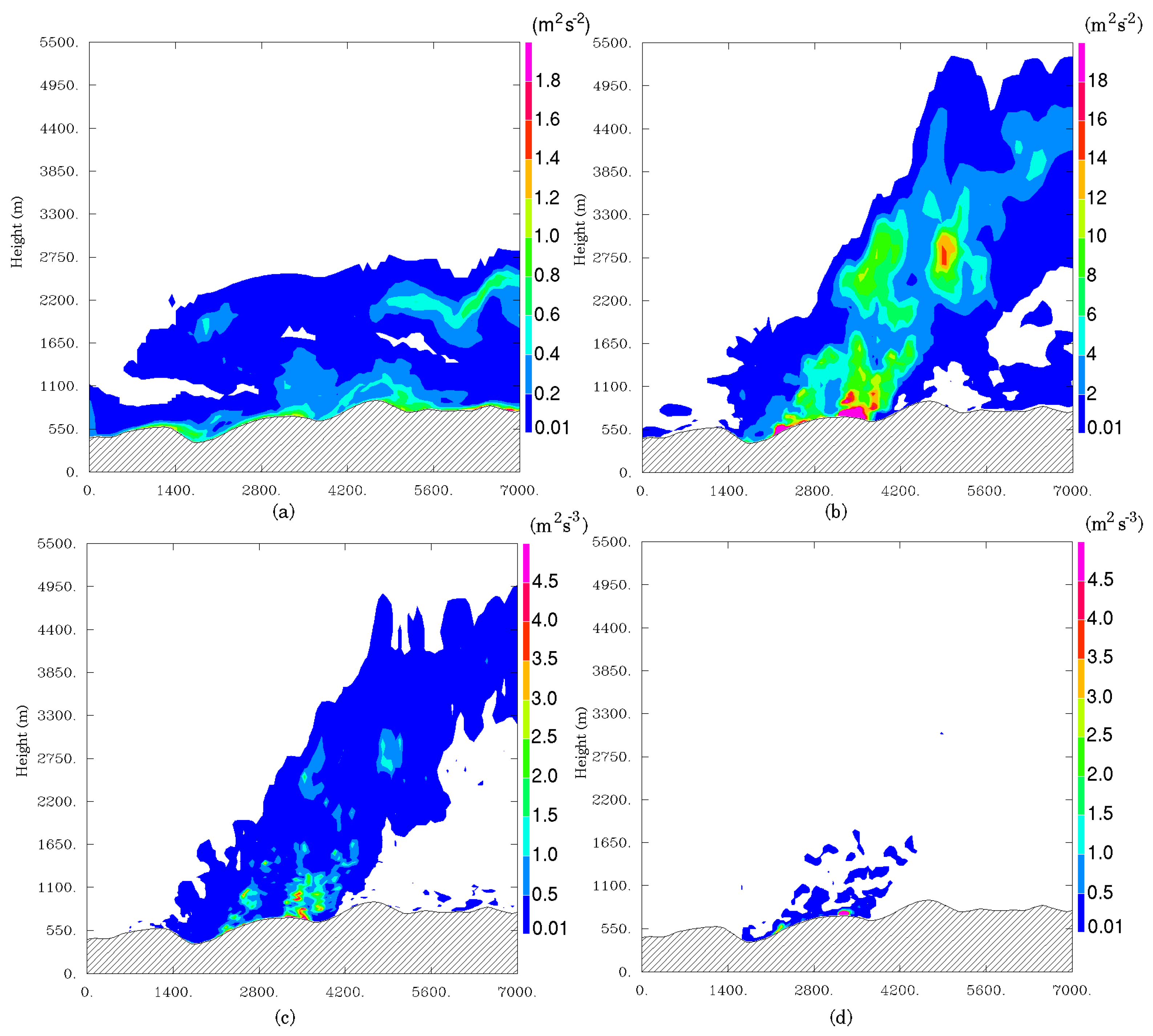
Vertical cross-sections along the direction of propagation (axis(A) in Figure 8a) on 23 July 2009 at 1500 UTC of Turbulent Kinetic Energy (TKE) (in ) for the (a) “uncoupled” and (b) the difference “coupled minus uncoupled” (with a ratio of 10 between isocontours); (c) dynamical production of TKE (in ) and (d) thermal production of TKE (in ) for the difference “coupled minus uncoupled”.
Figure 12.
Vertical cross-sections along the direction of propagation (axis(A) in Figure 8a) on 23 July 2009 at 1500 UTC of Turbulent Kinetic Energy (TKE) (in ) for the (a) “uncoupled” and (b) the difference “coupled minus uncoupled” (with a ratio of 10 between isocontours); (c) dynamical production of TKE (in ) and (d) thermal production of TKE (in ) for the difference “coupled minus uncoupled”.

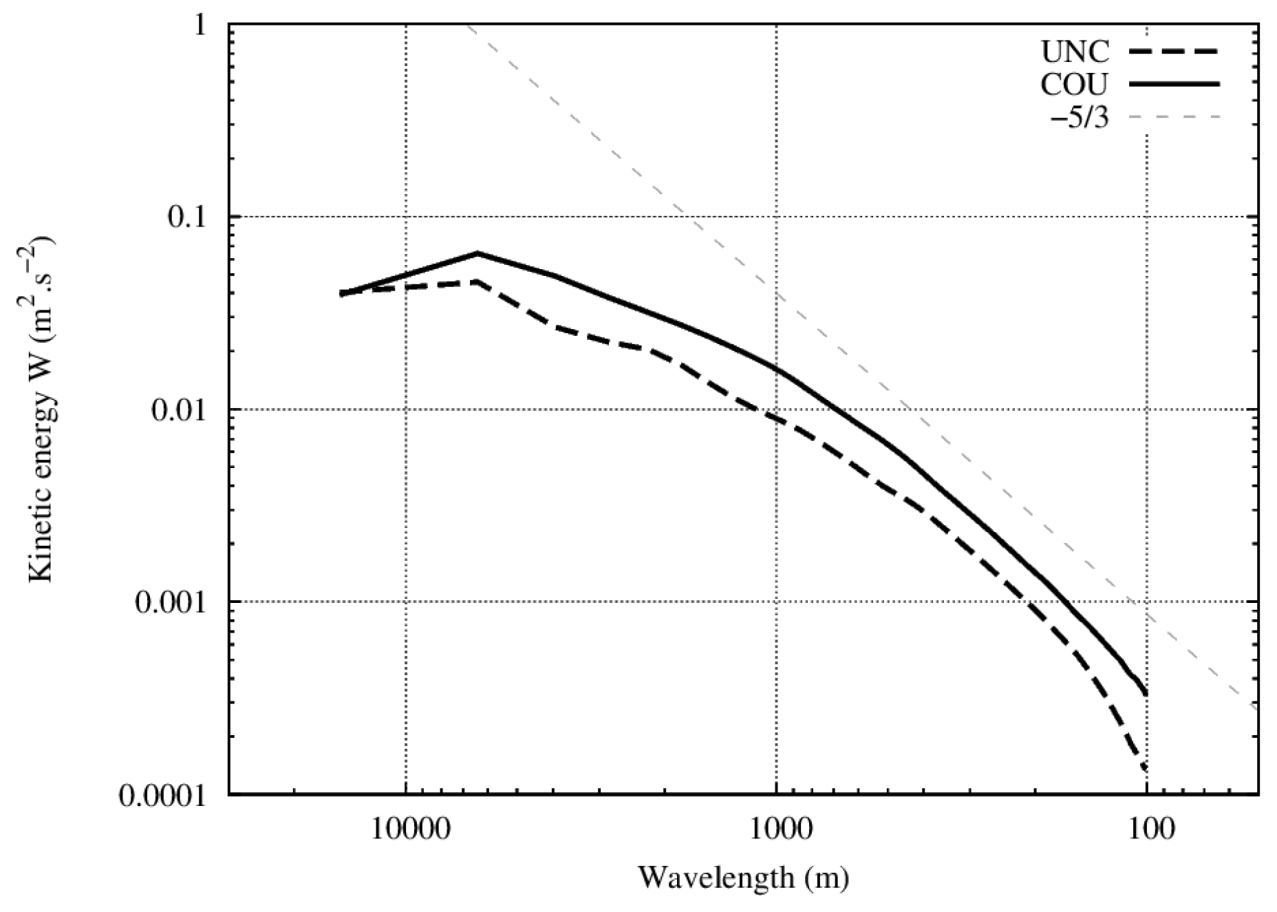
Figure 13.
Mean kinetic energy spectra for vertical wind on 23 July 2009 at 1500 UTC for the “Coupled” (continuous line) and “Uncoupled” (dashed line) simulations according to the wavelength (in m). The dashed line indicates the power law with an exponent of (the Kolmogorov spectrum).
Figure 13.
Mean kinetic energy spectra for vertical wind on 23 July 2009 at 1500 UTC for the “Coupled” (continuous line) and “Uncoupled” (dashed line) simulations according to the wavelength (in m). The dashed line indicates the power law with an exponent of (the Kolmogorov spectrum).

Figure 14.
“Coupled” simulation on 23 July 2009 at 1500 UTC: vertical cross-sections along the direction of propagation (axis in Figure 8a) of (a) zonal wind variance , (b) meridional wind variance and (c) vertical wind variance (in ).
Figure 14.
“Coupled” simulation on 23 July 2009 at 1500 UTC: vertical cross-sections along the direction of propagation (axis in Figure 8a) of (a) zonal wind variance , (b) meridional wind variance and (c) vertical wind variance (in ).

Figure 15.
“Fire-to-atm” simulation on 23 July 2009 at 1500 UTC: horizontal cross-sections of (a) the fire front (in black) at the ground superimposed on the wind vectors (arrows) and on the orography (color, in m); (b) the difference between “fire-to-atm” and “uncoupled” simulations of 10-m wind intensity with wind vectors superimposed (in ).


Table 1.
Main fuel types’ parameter values.
| Shrubs | Pine | Mixed | Maquis | |
|---|---|---|---|---|
| (kg·m) | 0.6 | 2 | 1.5 | 0.8 |
| E (m) | 0.5 | 3 | 2.5 | 2 |
| m (%) | 8 | 15 | 10 | 8 |
| (MJ·kg) | 18.6 | 16 | 17 | 18.6 |
Table 2.
Computation time for the different configurations.
| Exec. Time | Ratio | Overhead | |
|---|---|---|---|
| (for 6000 s) | (/Real Time) | (%) | |
| Uncoupled | 7550 | 1.26 | 0.00 |
| Fire-to-atm | 8700 | 1.45 | 15.23 |
| Coupled | 8240 | 1.37 | 9.14 |
| Coupled | 4580 | 0.76 | 9.14 |
| (depopulated) |
© 2018 by the authors. Licensee MDPI, Basel, Switzerland. This article is an open access article distributed under the terms and conditions of the Creative Commons Attribution (CC BY) license (http://creativecommons.org/licenses/by/4.0/).
Share and Cite
MDPI and ACS Style
Filippi, J.-B.; Bosseur, F.; Mari, C.; Lac, C. Simulation of a Large Wildfire in a Coupled Fire-Atmosphere Model. Atmosphere 2018, 9, 218. https://doi.org/10.3390/atmos9060218
AMA Style
Filippi J-B, Bosseur F, Mari C, Lac C. Simulation of a Large Wildfire in a Coupled Fire-Atmosphere Model. Atmosphere. 2018; 9(6):218. https://doi.org/10.3390/atmos9060218
Chicago/Turabian StyleFilippi, Jean-Baptiste, Frédéric Bosseur, Céline Mari, and Christine Lac. 2018. "Simulation of a Large Wildfire in a Coupled Fire-Atmosphere Model" Atmosphere 9, no. 6: 218. https://doi.org/10.3390/atmos9060218
Note that from the first issue of 2016, this journal uses article numbers instead of page numbers. See further details here.