Copula-Based Hazard Risk Assessment of Winter Extreme Cold Events in Beijing

Abstract

Extreme cold events (ECEs) have occurred more frequently over the last few winters in China, associated with large losses of human life and increasing costs. Here, copulas are used to establish a bivariate copula distribution model for ECE variables of duration and intensity, based on observed daily surface air temperatures in winter from 1978 to 2015 at 20 meteorological stations in Beijing. We demonstrate that durations of ECEs follow Weibull distributions, while their intensities fit a generalized extreme value distribution at most stations. The Gumbel–Hougaard copula best described the relationship between duration and intensity of ECEs at most stations. The joint and conditional return periods based on the bivariate copula described both ECE frequency and the corresponding hazard risk. A high risk was calculated for northern and western areas of Beijing, while a lower risk was calculated for urban and southeastern areas. Although the risk of a low temperature event of greater than 3 days with intensity in the range from −12 °C to −15 °C decreased, the risk of extreme low temperature events with durations greater than 2 days and intensity lower than −15 °C increased over the last 18 years. These probabilistic properties provide useful information for both climate change and hazard risk assessments.

1. Introduction

Arctic amplification (the greater warming of the Arctic compared with lower latitudes) is increasing the likelihood of the type of weather patterns that lead to mid-latitude cold extremes [1,2,3,4]. Cold extremes, which are becoming more likely under global warming, are associated with large losses of human life and exponentially increasing costs [5,6,7,8]. Thus, occurrences, characteristics, and risk evaluation of cold extremes have received increasing attention in recent decades [1,5,9,10].

Many previous studies have investigated the typical features and formation mechanisms of extreme cold events (ECEs) [7,11,12]. For example, Choi, et al. [11] examined the spatial and temporal patterns of changes in extreme events of temperature over the Asia-Pacific Network countries. Cholaw, et al. [12] discussed large-scale circulation features of ECEs. Zuo, et al. [5] and Sun, et al. [10] investigated the characteristics of ECEs in China. Honda, et al. [13] and Screen, et al. [1] discussed the determinants of the future risk of cold extremes. Although previous studies have paid much attention to cold extremes, there are few studies dealing with their probabilistic behavior or risk assessments.

Identifying the probabilistic behavior and risk of an ECE is crucial to an in-depth understanding of climatic mechanisms responding to climate changes, as well as providing evidence for forecasting of future climate-induced risks. Risk assessment of extreme events is typically carried out using the peaks over threshold (POT) extreme value analysis [14], a generalized extreme value (GEV) [15] distribution, or a percentile threshold method [16]. All these methods are probabilistic and based on univariate information, but can only be used for univariate statistical analysis of extreme temperature events. They cannot be used to analyze the multivariate characteristics of such events. An ECE is a multivariate phenomenon characterized by a temperature threshold, duration, and interval. It is difficult to make a comprehensive evaluation of the risk and probability of such cold extremes using only univariate information. The copula technique makes it possible to model dependence among multivariate data, independent of their marginal probability distributions. Thus, it allows multivariate random events to be described using different types of marginal distributions [17]. The copula function was initially introduced to explore abnormally high risks associated with insurance and finance, but has been widely used in studies of extreme events, such as drought [18], rainfall [19], and floods [20]. Previous studies have shown that the copula function can provide better multivariate joint distributions and an analysis of the frequency of related incidents. The corresponding return periods is a common criterion employed in the risk assessment of extreme events. The return period provides a very simple, yet efficient means for conducting risk analysis because it is able to concentrate a large amount of information into a single number [17]. Few studies have applied copula functions and the return periods to study ECEs.

Beijing, the capital of China, is an international metropolis; it will host the 2022 winter Olympics. Concurrent with the rapid expansion of the city and the rapid increase in population, the intensity and frequency of ECEs have increased. Anomalous cold winters are important ECEs that have adverse effects on industrial and agricultural production, people’s livelihoods, and social security. For instance, in 2004, a low temperature event occurred in Beijing in winter, which caused a severe heating energy shortage. The persistent extreme low temperature events in Beijing in November 2009 led to severe impacts on human life and the economy [21]. Clearly, there is a strong need to identify characteristics of cold extremes and a risk assessment through comprehensive analysis. Here, we attempt to study ECEs in Beijing using copulas. The principal aim of this study was to evaluate the risk of ECEs in Beijing using copula functions and provide useful information for both climate change and risk assessments. The remainder of this paper is organized as follows. Section 2 describes the study area and the data used. The method used to establish a bivariate copula distribution model for ECE variables is presented in Section 2. The results of the copula and risk analysis for ECEs are given in Section 3. Finally, our conclusions are stated in Section 4.

2. Materials and Methods

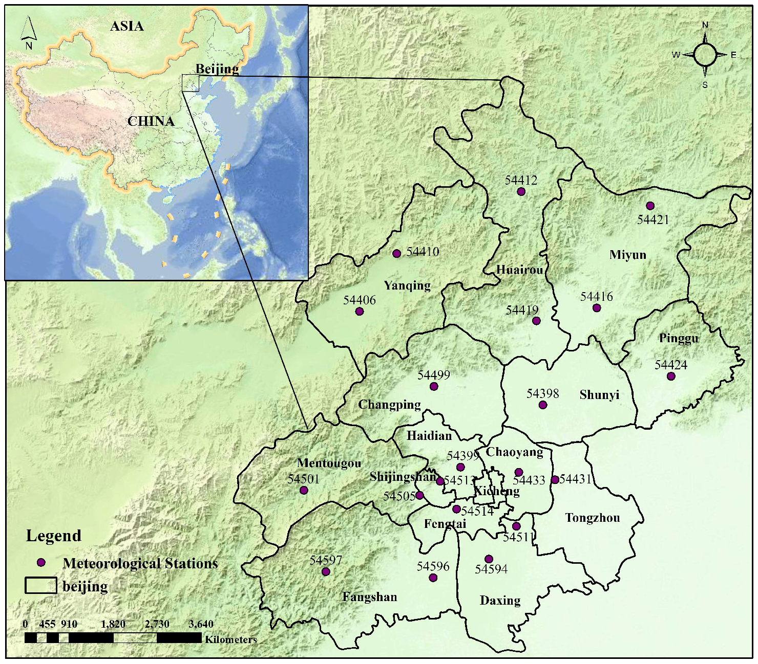
2.1. Descriptions of Study Area and Meteorological Data

Beijing was selected as the study area. The city borders the North China Plain and the Inner Mongolia Plateau; it is surrounded by the Taihang Mountains on the west and the Yanshan Mountains to the north (Figure 1). Beijing is influenced by the Siberian anticyclone, which brings colder, windier, and drier winters. The minimum absolute temperature can be lower than −20 °C in bitterly cold winters.

The observational daily mean 2-m temperature (T2m) data from 20 meteorological stations in Beijing were used in this study (

Table 1. Information on stations and their locations used in the study.

Station Identity (ID)	Name	Longitude (°)	Latitude (°)	Elevation (m)
54398	Shunyi	116.37	40.8	28.6
54399	Haidian	116.17	39.59	45.8
54406	Yanqing	115.58	40.27	487.9
54410	Foyeding	116.08	40.36	1224.7
54412	Tanghekou	116.38	40.44	331.6
54416	Miyun	116.52	40.23	71.8
54419	Huairou	116.38	40.22	75.7
54421	Shangdianzi	117.07	40.39	293.3
54424	Pinggu	117.07	40.10	32.1
54431	Tongzhou	116.38	39.55	43.3
54433	Chaoyang	116.30	39.57	35.3
54499	Changping	116.13	40.13	76.2
54501	Zhaitang	115.41	39.58	440.3
54505	Mentougou	116.07	39.55	92.7
54511	Beijing	116.28	39.48	31.3
54513	Shijingshan	116.12	39.57	65.6
54514	Fengtai	116.15	39.52	55.2
54594	Daxing	116.21	39.43	37.6
54596	Fangshan	116.08	39.41	39.2
54597	Xiayunling	115.44	39.44	407.7

, Figure 1). The meteorological data are provided by the Chinese Meteorological Administration, which carries out data quality checks. The data for December, January, and February for the period 1978–2015 were used. There were a few missing values in the daily temperature data sets, although missing values comprised less than 0.01% of the total values. These missing values were filled using the average values of neighboring days. This gap filling method has no influence on long-term temporal trends. Locations and elevations of meteorological stations are given in Table 1. These stations are sparsely distributed in mountainous areas, but are densely distributed on the plain, especially within urban areas.

2.2. Selection of Extreme Cold Events

Exposure to −15 °C can result in frostbite, while long outdoor exposure to −10 °C can result in freezing of superficial tissues. In this study, ECEs were divided into low temperature events and extreme low temperature events. A low temperature event occurs when the daily mean temperature falls below −10 °C but is above −15 °C, while an extreme low temperature event occurs when the daily mean temperature falls below −15 °C. In previous studies, cold extremes were described by few parameters: frequency, duration or length, severity, and/or intensity [22,23,24]. The principal aim of this study was the risk assessment of ECEs that can provide useful information to help the 2022 Winter Olympics. Therefore, the ECEs with long lasting times and extreme low temperatures should be paid more attention. In this study, for each ECE, we assigned a duration and an intensity. Duration refers to the number of days the event lasted, while intensity is computed as the mean temperature over the entire event.

Subsequently, over the period from 1978 to 2015, we computed the frequency of occurrence, maximum duration, and average intensity of ECEs at each station. The maximum duration refers to the maximum time these events lasted, while all averaged quantities refer to the average value computed for events occurring over an entire year.

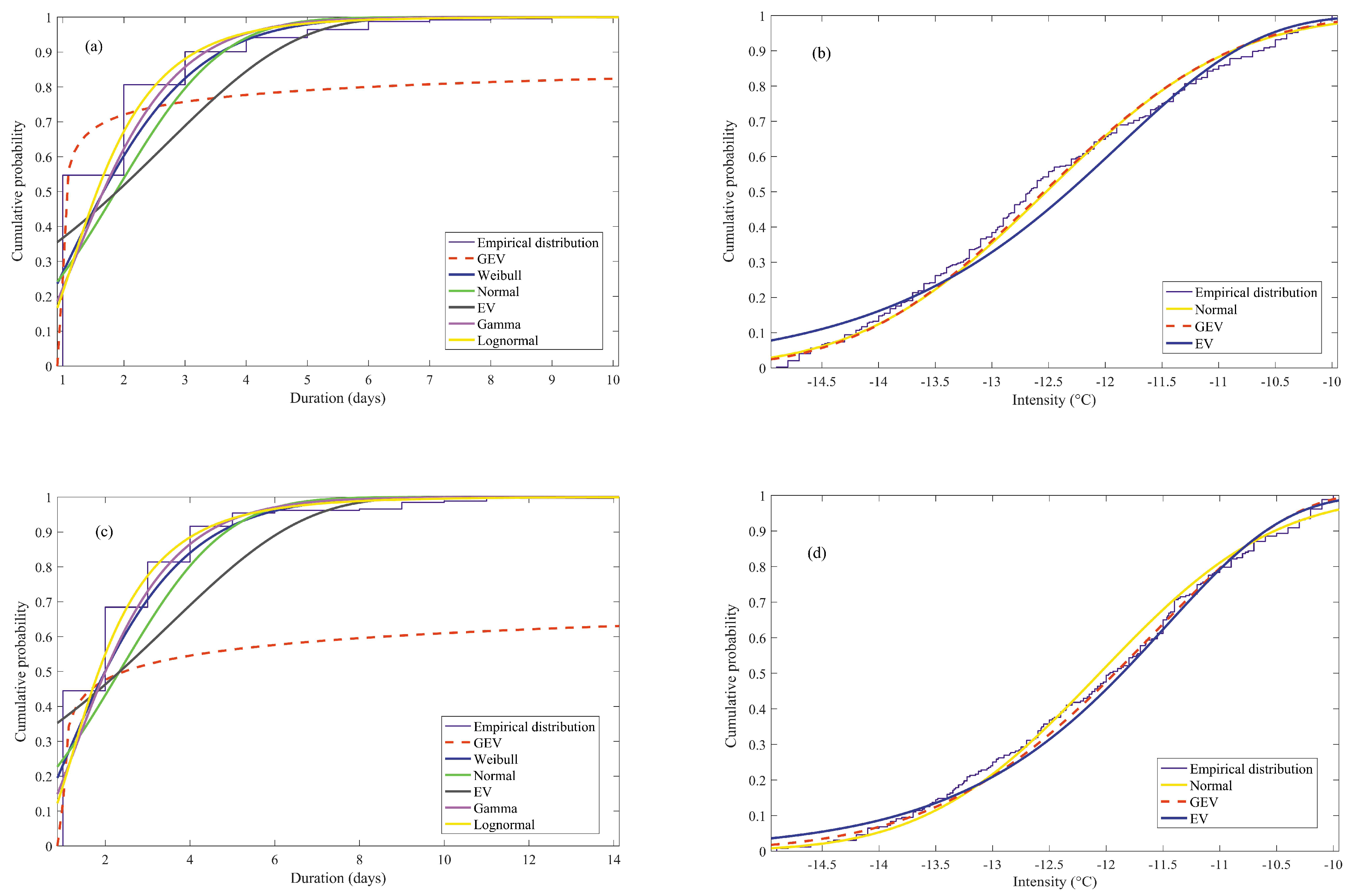
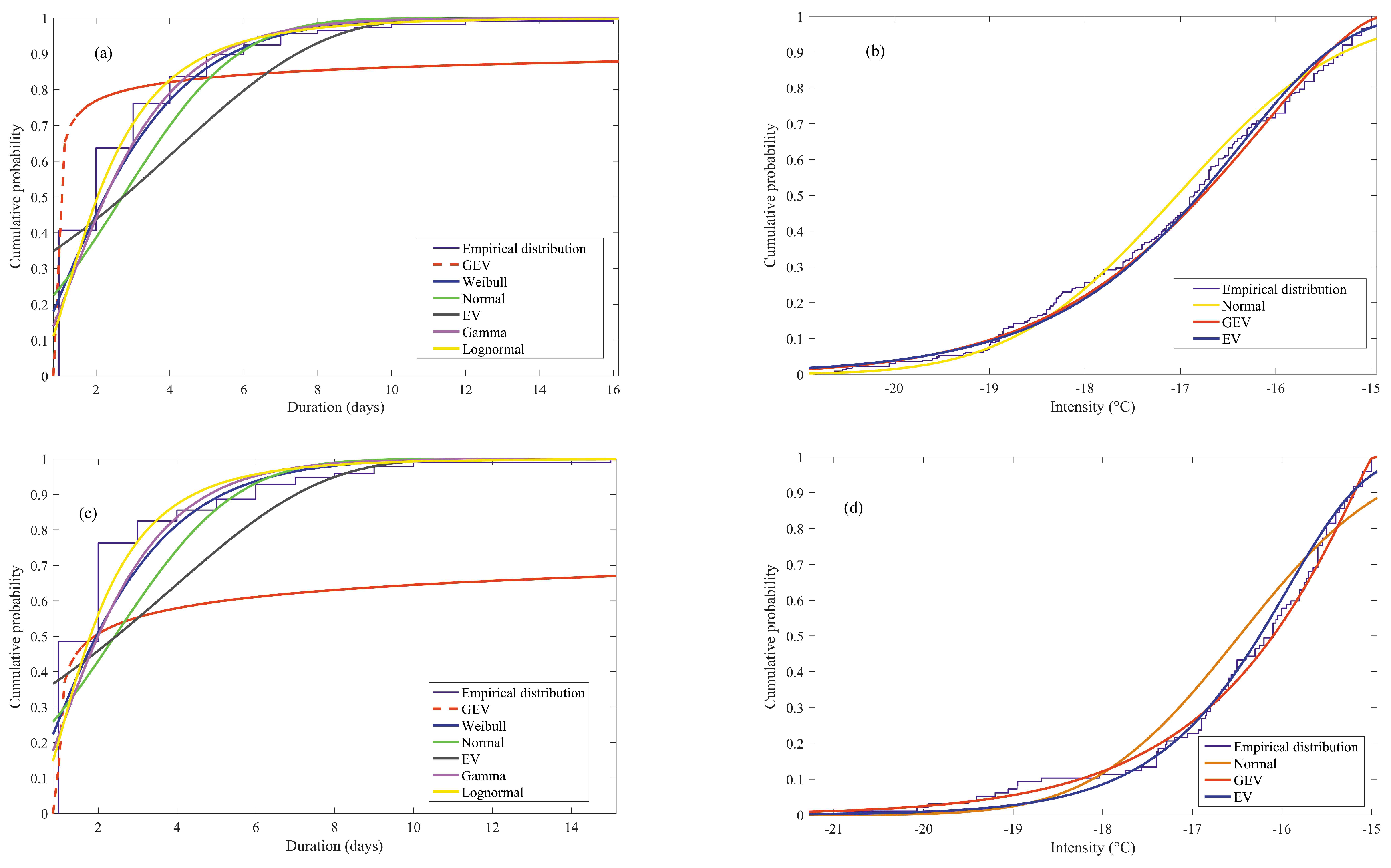
2.3. Estimation of Marginal Probability Distributions

Marginal distributions of ECE duration and intensity were analyzed using a conventional univariate approach for each station. Six distributions were employed, including normal, gamma, generalized extreme value (GEV), extreme value (EV), three-parameter lognormal, and Weibull distributions. Parameters for these distribution functions were estimated using maximum likelihood estimation. The goodness-of-fit of the probability function was evaluated using the Kolmogorov–Smirnov (K–S) test [25] at a >90% confidence level. The probability distribution function having the best goodness-of-fit with observational data was selected for each station.

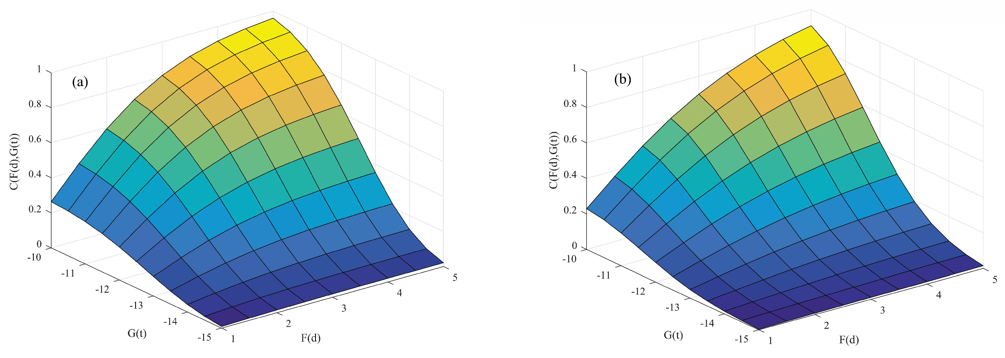
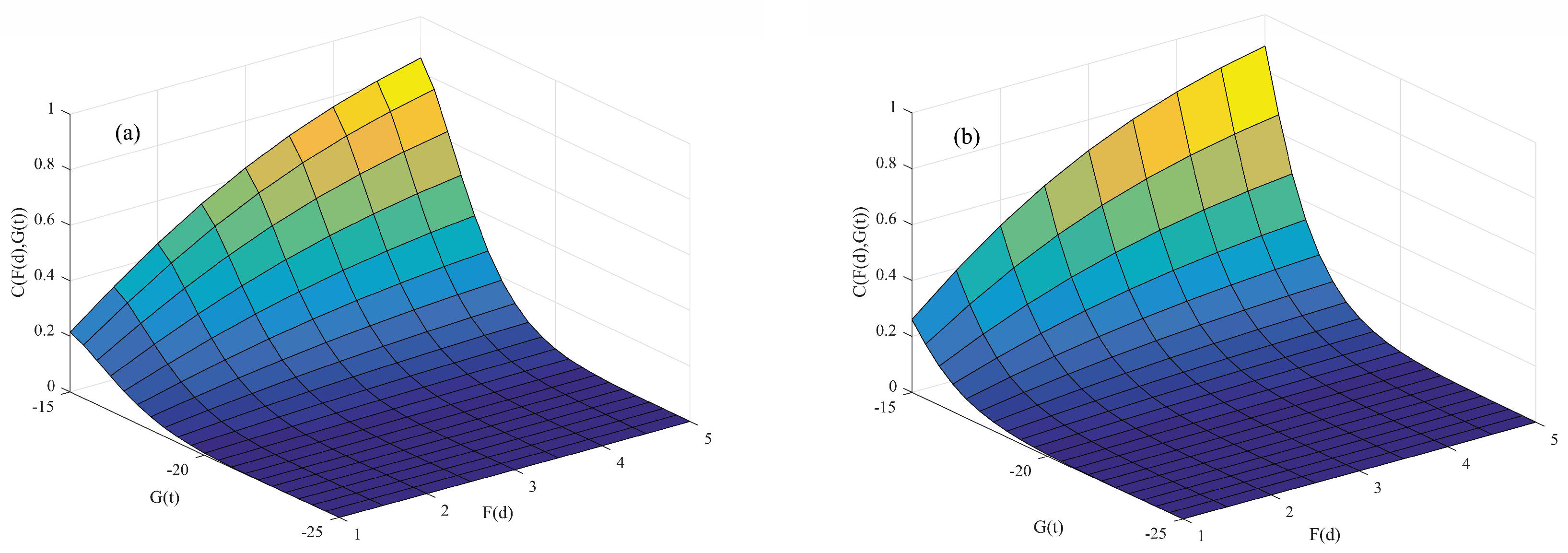
2.4. Copula Functions

Sklar [26] showed that if two random variables x and y follow arbitrary marginal distribution functions $F_X(x)$ and $F_Y(y)$, then there exists a copula C to combine these two marginal distribution functions, as follows:

$$F_{X,Y}(x,y)=C(F_X(x),F_Y(y))$$

(1)

where the function $F_{X,Y}(x,y)$ is a two-dimensional distribution function with marginal distributions $F_X(x)$ and $F_Y(y)$. If the marginal distribution $F_X(x)$ and $F_Y(y)$ are continuous, then the copula function C is unique, and the joint probability density function can be written as follows:

$$f_{X,Y}(x,y)=c(F_X(x),F_Y(y))f_X(x)f_Y(y)$$

(2)

where $f_X(x)$ and $f_Y(y)$ denote the density functions corresponding to $F_X(x)$ and $F_Y(y)$, respectively. In this case, c is the density function of C, expressed as follows:

$$c(u,v)=\frac{{\partial }^{2}C(u,v)}{\partial u\partial v}$$

(3)

where u and v denote the cumulative distribution functions, that is, $F_X(x)$ and $F_Y(y)$, in Equations (1) and (2), the values of which range from zero to one.

Copulas provide a convenient way to separately fit each variable to a marginal distribution and then join them together. Multivariate normality is only one option in a wide range of copula-based models that can capture the principal features of variable data, such as non-symmetry, nonlinear dependence, or heavy-tail behavior. There are numerous different copulas to choose from, with various correlation properties such as symmetry, tail dependence, and range of dependence [27].

2.4.1. Bivariate Archimedean Copulas

In this study, the Archimedean copulas (

Table 2. Formulas of various copulas and their parameter estimation. GH—Gumbel–Hougaard.

Copula Type	Function
Clayton	$C(u,v)={(u^{-\theta }+v^{-\theta }-1)}^{-1/\theta }$
GH	$C(u,v)=\exp \{-{[{(-\ln u)}^{\theta }+{(-\ln v)}^{\theta }]}^{1/\theta }\}$
Frank	$C(u,v)=-\frac{1}{\theta }\ln [1+\frac{(e^{-\theta u}-1)(e^{-\theta v}-1)}{e^{-\theta }-1}]$

), including Clayton, Gumbel–Hougaard (GH), and Frank copulas, were selected to analyze the joint probability of ECEs because of their simplicity and wide representation [28,29]. The copula parameter $\theta$ is used to measure the degree of association between u and v. The inference functions for the marginal distribution method (IFM) proposed by Joe (1997) [30] employed for fitting copulas involves estimating the parameters of the copula. The IFM is a fully parametric method, so the misspecification of the marginal distributions may affect the performance of this estimator. Thus, the joint distribution is estimated expeditiously by the marginal distributions and the parameters in the copula function are estimated using these maximum likelihood values individually. As noted by Joe (2005) [31], use of the technique can prevent computational difficulty for high dimensional models in the maximum likelihood estimation where the marginal distribution parameters and the copula parameters are estimated simultaneously.

2.4.2. Goodness-of-Fit Tests for Copula Functions

Copula functions were evaluated using an empirical copula function [28]. This empirical copula was defined as follows:

$$C_e(u,v)=\frac{1}{n}{\displaystyle \sum _{i=1}^n{I}_{[F_n(x_i\le u]}{I}_{[H_n(y_i\le v)]}},\begin{array}{cc}& \end{array}u,v\in [0,1]$$

(4)

where $x_i$, $y_i$ (i=1, 2,…, n) are samples from a two-dimensional distribution; n is the sample size; and (X, Y), $F_n(x)$, and $H_n(y)$ are the empirical distribution functions of X and Y, respectively. Here, $I_{[•]}$ is the indicator function; when $F_n(x_i)\le u$, $I_{[F_n(x_i)\le u]}=1$, otherwise $I_{[F_n(x_i)\le u]}=0$. The root-mean-square error (RMSE) was used to estimate the degree-of-fit between the empirical copula and the theoretical copula [32]. The RMSE can be written as follows:

$$RMSE=\sqrt{\frac{1}{n}{\displaystyle \sum _{i=1}^n{[C_p(i)-C_e(i)]}^2}}$$

(5)

where n is the sample size, $C_p$ denotes the computed values of the theoretical copula, and $C_e$ denotes the observed values of the probability obtained from the empirical copula. The copula function with the lowest RMSE value was selected at each station.

2.5. Return Periods

The return period and related probability distributions were derived for risk assessment. In this study, the return periods for a bivariate distribution can be defined in two ways. The first method defines the joint return periods using one random variable equaling or exceeding a certain magnitude and/or another random variable equaling or exceeding another given magnitude. The second method defines the conditional return periods for one random variable given that another random variable equals or exceeds a specific value [33].

The two variables describing both types of ECEs are duration and intensity. Low temperature/extreme low temperature events with long durations and low temperatures may have a considerable influence on human society. In this case, the joint events considered in this study are the following:

$$\{D>d\}\wedge \{T<t\}$$

(6)

Let D denote the duration and T the intensity, then joint return periods related to these two events can be computed using the following:

$$R_{\{D>d\wedge T<t\}}=\frac{\mu }{P(D>d\wedge T<t)}=\frac{\mu }{G(t)-C(F(d),G(t))}$$

(7)

where $\wedge$ denotes “and”, and $R_{\{D>d\wedge T<t\}}$ denotes the joint return period when D exceeds the specific threshold and T is less than the specific threshold; $P(D>d\wedge T<t)$ denotes the probability of this event; and G(t) and F(d) are the marginal distribution functions of intensity and duration, respectively. In this case, $\mu$ denotes the mean time interval between two successive events, with the unit of $\mu$ defined as a year in this study [17].

The conditional probability of ECEs describes the possibility of certain extreme cold episodes. The conditional return period of ECEs, when the given duration exceeds a certain threshold, is given by the following:

$$R_{\{T<t|D>d\}}=\frac{\mu }{P(T<t|D>d)}=\frac{\mu }{\frac{G(t)-C(F(d),G(t))}{1-F(d)}}$$

(8)

and the conditional return period of ECEs with a given intensity threshold is expressed as follows:

$$R_{\{D>d|T<t\}}=\frac{\mu }{P(D>d|T<t)}=\frac{\mu }{1-\frac{C(F(d),G(t))}{G(t)}}$$

(9)

Return periods were interpolated to cover the whole area of Beijing using inverse distance weighted (IDW) interpolation [34]. The risks of low temperature and extreme low temperature events, respectively, were evaluated in this study. To analyze the changes in risk characteristics for these two types of ECEs, data from 1978 to 2015 of each event were divided into two periods, covering from 1978 to 1998 and from 1999 to 2015.

3. Results

3.1. Low Temperature Events

3.1.1. Statistics of Low Temperature Events

The frequency, maximum duration, and mean intensity of low temperature events for each station are presented in

Table 3. Statistics of low temperature events for 20 meteorological stations in Beijing.

Stations		Frequency		The Maximum Duration (Days)		Mean Intensity (°C)
ID	Name	1978–1998	1999–2015	1978–1998	1999–2015	1978–1998	1999–2015
54398	Shunyi	148	97	13	12	−11.53	−11.43
54399	Haidian	170	105	7	6	−11.35	−11.31
54406	Yanqing	393	263	10	14	−12.52	−12.06
54410	Foyeding	323	255	9	8	−12.45	−12.32
54412	Tanghekou	354	288	10	10	−12.60	−12.68
54416	Miyun	311	239	14	9	−11.97	−11.87
54419	Huairou	180	196	8	13	−11.56	−11.92
54421	Shangdianzi	310	266	10	12	−12.09	−12.06
54424	Pinggu	319	208	10	15	−11.97	−11.74
54431	Tongzhou	196	51	10	9	−11.66	−11.17
54433	Chaoyang	187	103	10	8	−11.48	−11.28
54499	Changping	211	96	11	8	−11.48	−11.41
54501	Zhaitang	379	288	9	10	−12.14	−12.13
54505	Mentougou	184	102	10	9	−11.49	−11.51
54511	Beijing	138	74	6	8	−11.36	−11.31
54513	Shijingshan	159	70	14	8	−11.57	−11.14
54514	Fengtai	194	105	11	8	−11.35	−11.43
54594	Daxing	198	104	9	8	−11.66	−11.41
54596	Fangshan	223	135	9	6	−11.81	−11.71
54597	Xiayunling	176	125	13	13	−11.37	−11.64

. Clearly, there are regional difference in frequency. Zhaitang station, with 666 ECE occurrences, had the highest frequency. Generally, low temperature events occurred more often during the period 1978–1998 than during the period 1999–2015. For example, at Yanqing station, 393 events occurred before 1998, while 263 events occurred after 1998.

The maximum duration of ECEs at each station in Beijing averaged 10 d. The longest events were recorded at Miyun station, with a low temperature event lasting 14 days in 1978–1998, and at Pinggu station, with a low temperature event lasting 14 days in 1999–2015. There was little difference in the mean intensity of ECEs among stations. For example, the mean intensity of 148 events at Shunyi station from 1978 to 1998 was −11.53 °C, while the mean intensity of 170 events at Haidian station from 1978 to 1998 was −11.35 °C. For all stations, the mean intensity of events for the period 1999–2015 was lower than for the period 1978–1998. Both frequency and mean intensity were higher from 1978 to 1998 than from 1999 to 2015, which suggests that frequency and intensity of winter low temperature events are in decline.

3.1.2. Joint Distribution of Winter Low Temperature Based on the Copula Function

Yanqing station (ID 54506) was selected as a case study, with the aim to verify computations using the copula function in this study. Yanqing was selected for illustration because some new venues planned for the 2022 Winter Olympic will be built here and the ECEs are important for the Olympic Games. The goodness-of-fit of the marginal distributions for duration and intensity of low temperature events at Yanqing station were evaluated (Figure 2). Using the K–S test, the optimal probability distributions for duration and intensity for 20 stations in Beijing were determined. These distributions are listed in

Table 4. The goodness-of-fit based on the Kolmogorov–Smirnov (K–S) D statistic for marginal distributions of duration and intensity for low temperature events at 20 meteorological stations in Beijing. EV—extreme value; GEV—generalized EV.

Stations		The Period 1978–1998				The Period 1999–2015
		Duration		Intensity		Duration		Intensity
ID	Name	K–S D	Distributions	K–S D	Distributions	K–S D	Distributions	K–S D	Distributions
54398	Shunyi	0.1318	Weibull	0.0796	GEV	0.1246	Weibull	0.0799	GEV
54399	Haidian	0.1228	Weibull	0.0706	EV	0.1255	EV	0.1080	EV
54406	Yanqing	0.0789	Weibull	0.0544	GEV	0.1001	Weibull	0.0463	GEV
54410	Foyeding	0.0905	Weibull	0.0406	GEV	0.1019	Normal	0.0511	Normal
54412	Tanghekou	0.0872	Normal	0.0402	Normal	0.0954	Weibull	0.0394	GEV
54416	Miyun	0.0928	Normal	0.0522	GEV	0.1043	Normal	0.0451	GEV
54419	Huairou	0.1210	Weibull	0.0697	EV	0.1118	Weibull	0.0581	GEV
54421	Shangdianzi	0.0924	Weibull	0.0413	GEV	0.0950	Weibull	0.0371	GEV
54424	Pinggu	0.0909	Normal	0.0422	GEV	0.1112	Weibull	0.0668	GEV
54431	Tongzhou	0.1061	Weibull	0.0852	GEV	0.1005	Weibull	0.1388	Normal
54433	Chaoyang	0.1155	Weibull	0.0647	GEV	0.1532	Weibull	0.0944	GEV
54499	Changping	0.1107	Weibull	0.0742	Normal	0.1601	Weibull	0.0708	GEV
54501	Zhaitang	0.0836	Weibull	0.062	GEV	0.0907	Weibull	0.0467	GEV
54505	Mentougou	0.1134	Weibull	0.0682	GEV	0.1602	Weibull	0.0890	GEV
54511	Beijing	0.1373	Weibull	0.0683	GEV	0.1447	Weibull	0.0764	EV
54513	Shijingshan	0.1229	Weibull	0.0614	GEV	0.1696	Weibull	0.0873	EV
54514	Fengtai	0.1128	Weibull	0.0675	GEV	0.1104	Weibull	0.0844	Normal
54594	Daxing	0.1159	Normal	0.0635	GEV	0.1580	Normal	0.0681	GEV
54596	Fangshan	0.1084	Weibull	0.0494	GEV	0.1360	Weibull	0.0948	GEV
54597	Xiayunling	0.1224	Gamma	0.0736	GEV	0.1340	Weibull	0.0710	Normal

.

There were 393 and 263 low temperature events recorded at Yanqing station during the periods 1978–1998 and 1999–2015, respectively. At a 90% confidence level, the K–S test yielded D values of 0.0822 and 0.1005, respectively [25]. To model the intensity of these events, all probability distributions performed well, although the GEV distribution best fitted the observed data. However, duration of these events was only modeled by the Weibull distribution, based on the K–S test (Figure 2).

Similar results were found for the other 19 stations in Beijing (Table 4). Typically, for event duration, only one or two distributions passed the K–S test, with marginal distributions of duration best fitted by the Weibull distributions at the majority of stations. At a few stations, such as Miyun and Daxing, only the normal distribution passed the K–S test; while at Xiayunling station, only the gamma distribution passed the K–S test for the period 1978–1998. In the case of intensity, the GEV distribution performed well for most stations. At the Haidian station, an EV distribution performed better than other distributions in both study periods. In general, the marginal distributions of duration and intensity of low temperature events were best fitted by the Weibull and GEV distributions, respectively.

After selecting the best-fit marginal distribution functions, the parameters of each copula function were computed. The copula families were determined based on RMSE values. The copula that produced the least error (lowest RMSE) was selected (

Table 5. Parameter estimation and root-mean-square error (RMSE) for selected copula distributions for 20 meteorological stations in Beijing.

Stations		1978–1998			1999–2015
ID	Name	$\mathit{\theta }$	RMSE	Copula	$\mathit{\theta }$	RMSE	Copula
54398	Shunyi	1.0135	0.0883	GH	1.0001	0.0886	GH
54399	Haidian	1.0001	0.0122	GH	−2.2989	0.0506	Frank
54406	Yanqing	0.1197	0.0154	Clayton	1.0000	0.0807	GH
54410	Foyeding	0.3651	0.0107	Clayton	0.1610	0.0150	Clayton
54412	Tanghekou	0.2985	0.0144	Clayton	0.3024	0.1158	Clayton
54416	Miyun	1.0000	0.1048	GH	1.0000	0.0150	GH
54419	Huairou	1.0136	0.0871	GH	1.0001	0.1030	GH
54421	Shangdianzi	0.0118	0.0921	Clayton	0.0310	0.1156	Clayton
54424	Pinggu	1.0000	0.1062	GH	1.0000	0.0855	GH
54431	Tongzhou	1.0001	0.0775	GH	1.0000	0.0174	GH
54433	Chaoyang	1.0013	0.0166	GH	1.0013	0.0168	GH
54499	Changping	1.4500	0.1061	GH	1.0001	0.0218	GH
54501	Zhaitang	−0.9643	0.0979	Frank	−1.3006	0.0997	Frank
54505	Mentougou	1.0001	0.1091	GH	1.0000	0.1090	GH
54511	Beijing	1.0017	0.1114	GH	1.0000	0.1084	GH
54513	Shijingshan	1.0000	0.0849	GH	1.0000	0.0130	GH
54514	Fengtai	1.0001	0.1046	GH	−2.3676	0.0247	Frank
54594	Daxing	−2.0774	0.1111	Frank	1.0000	0.1094	GH
54596	Fangshan	1.0000	0.0933	GH	−1.8516	0.0190	Frank
54597	Xiayunling	−2.6704	0.0870	Frank	1.0001	0.0616	GH

). According to Table 5, the GH copula provided the best-fit joint distribution for duration and intensity at most stations. The Frank copula was the best-fit for only three stations during the period 1978–1998, but four stations during the period 1999–2015. The Clayton copula distribution was selected for few stations, including Foyeding and Tanghekou stations, suggesting that the distributions of low temperature events may be regionally specific.

For the marginal distributions of the intensity and duration of low temperature events, the joint cumulative distribution function for the Yanqing station is shown in Figure 3. In the next section, these joint distributions are used to predict the return periods of winter low temperature events.

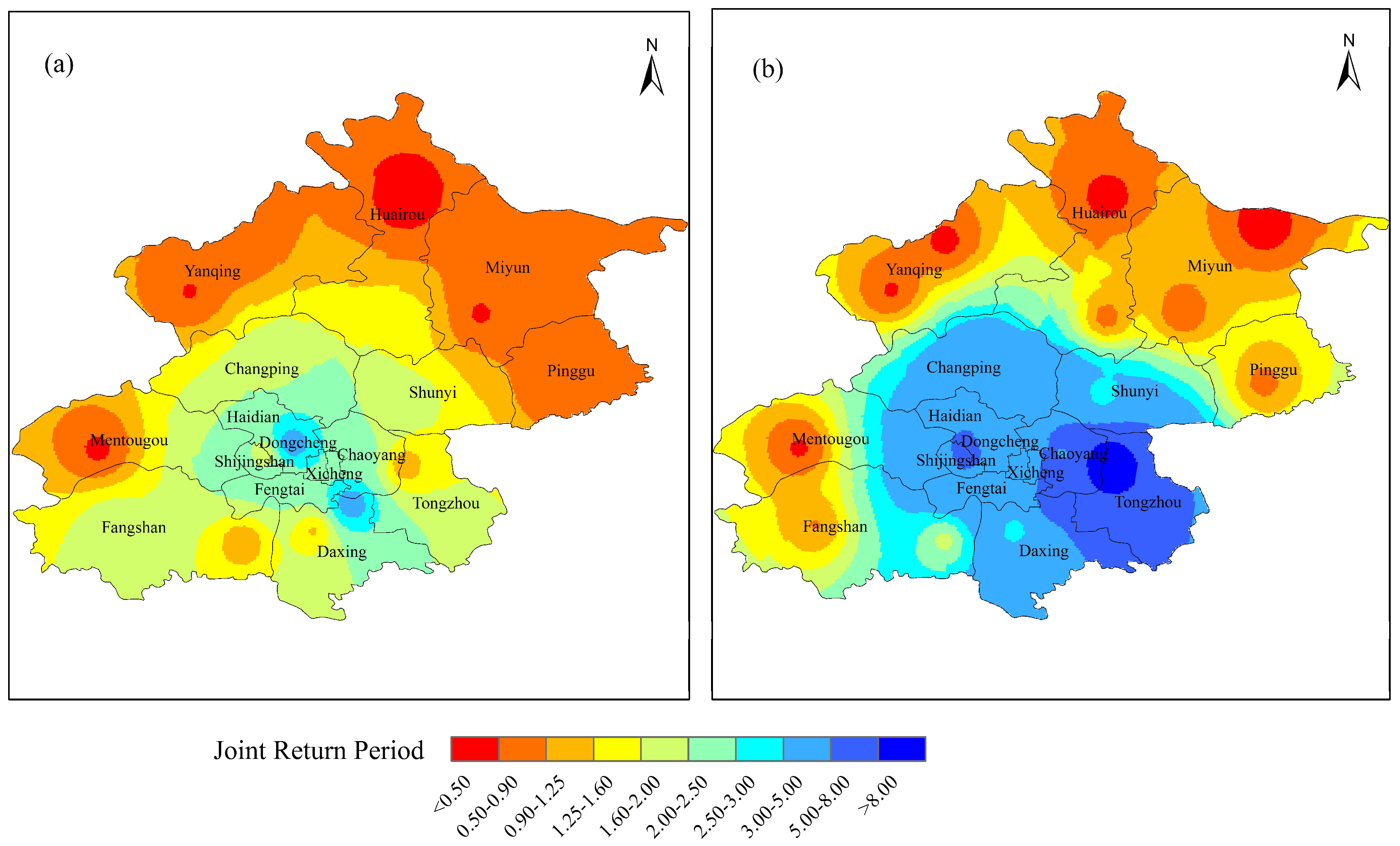
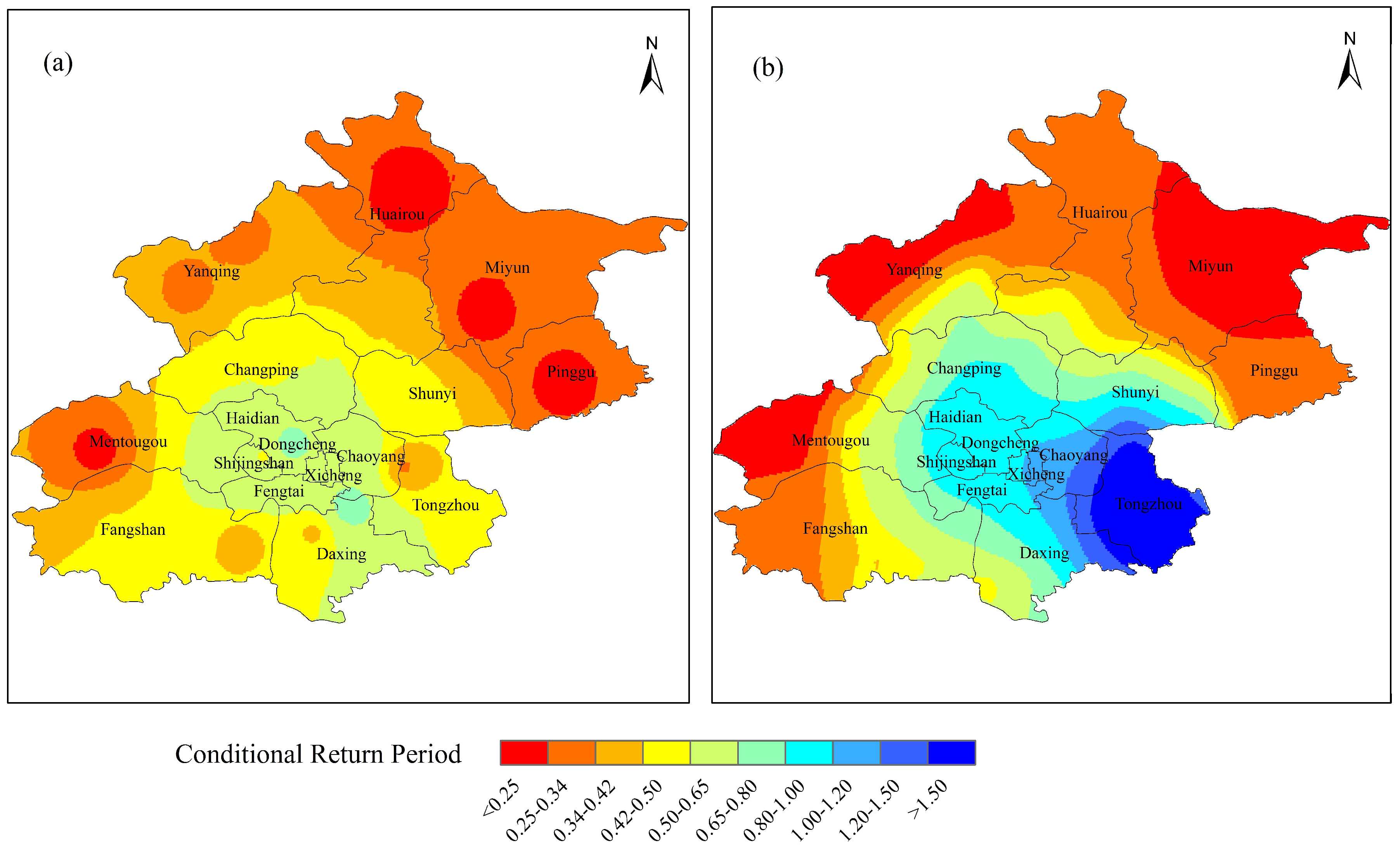
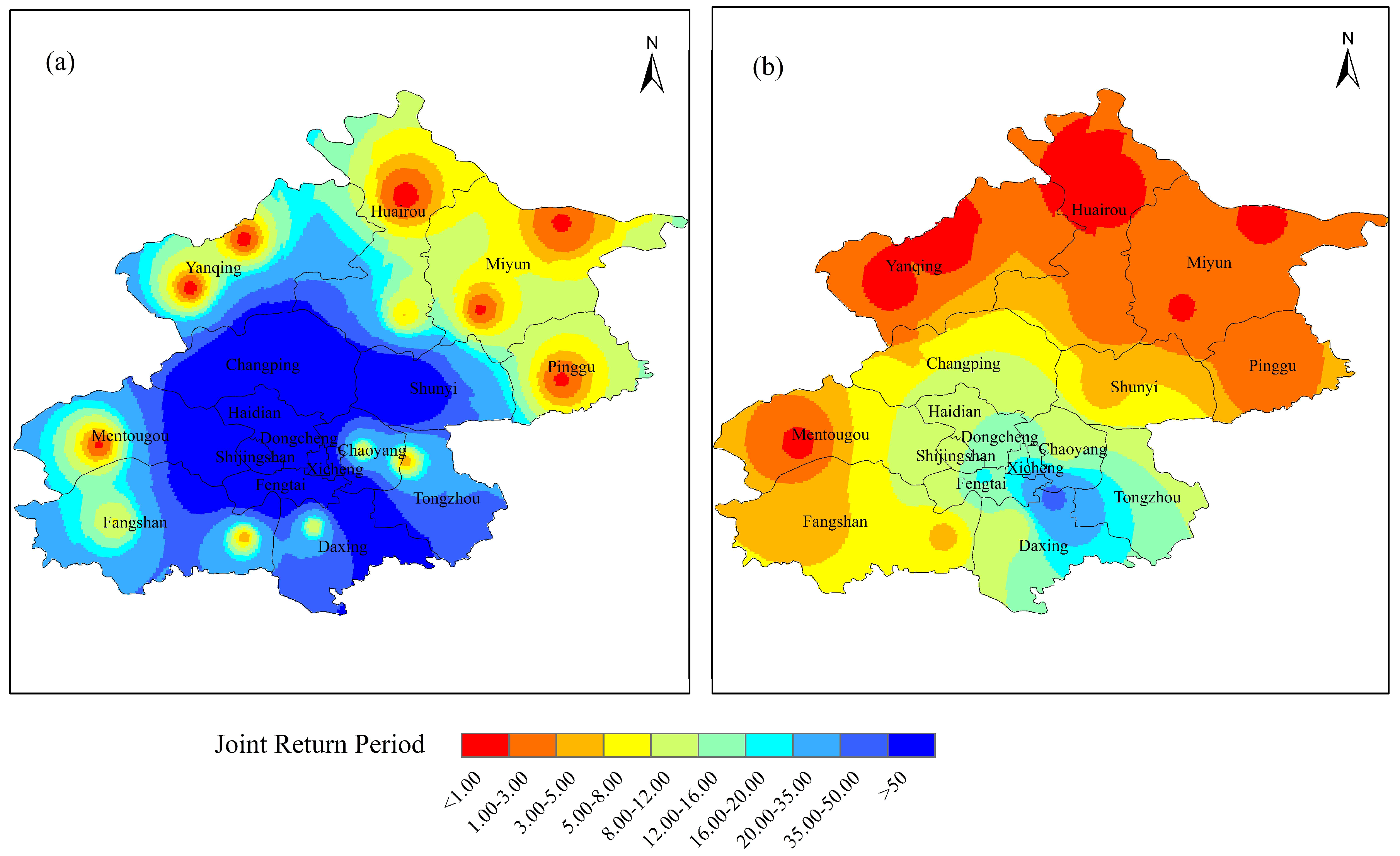
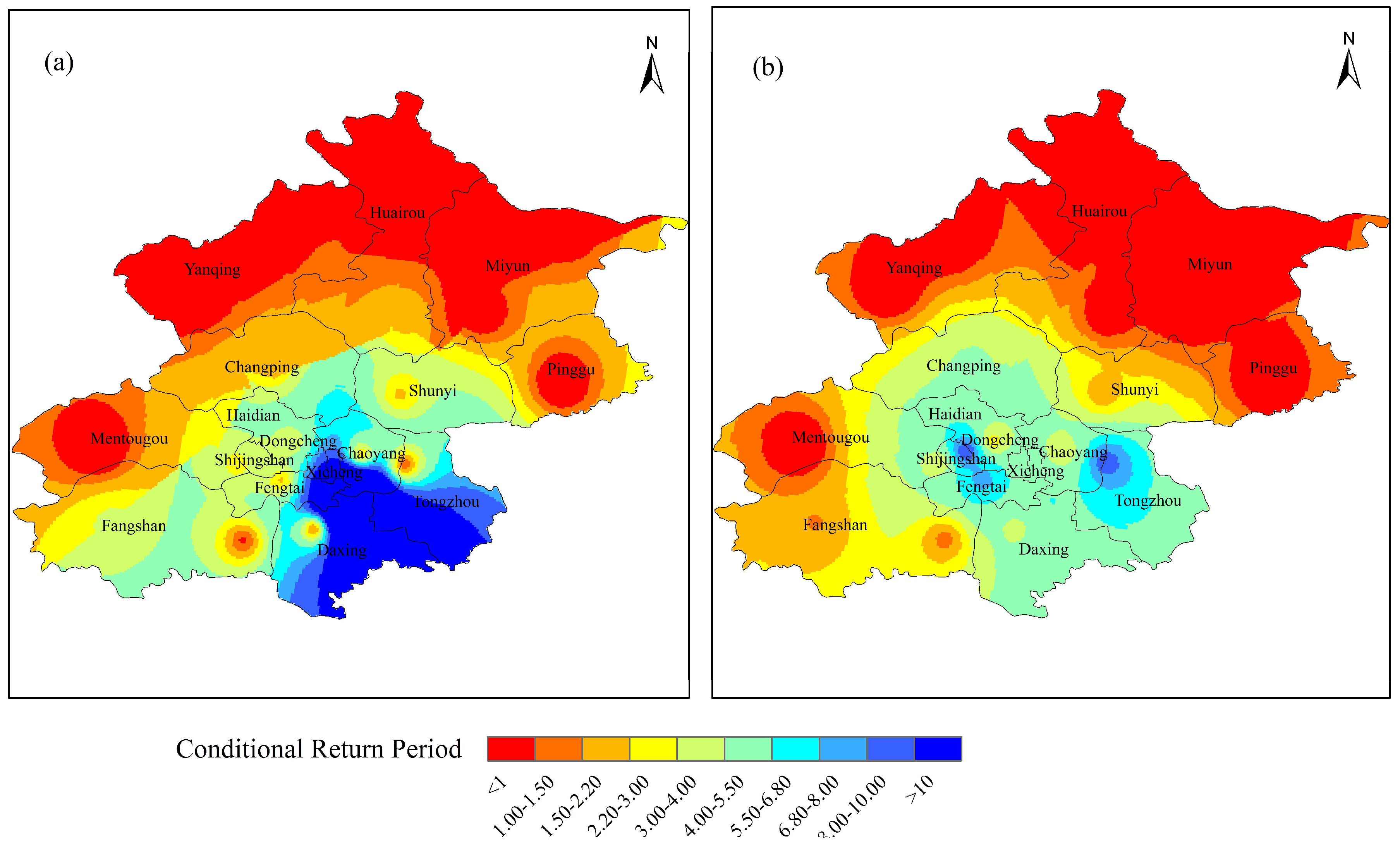
3.1.3. Return Period and Risk Analysis

Here, we consider only one scenario in our analysis of joint return periods, that is, the duration of events greater than 3 days duration with an intensity below −12 °C but above −15 °C. The results of the joint return period (Figure 4) suggest there is spatiotemporal variation to the risk of low temperature events within the study area.

Larger joint return periods imply a smaller probability that low temperature events will occur, and vice versa. Figure 4a,b show similar spatial patterns to return periods for both study periods. The highest low temperature risk was calculated for areas north and west of Beijing. Return periods exhibited a northeast–southwest trend, consistent with the topography of the Beijing region (Figure 1). This indicates that under the influence of topography, low temperature events occur more frequently in the northern and western mountainous areas of Beijing and less frequently on the plain.

Comparison of Figure 4a,b shows a general decrease in the risk of low temperature events after 1999, particularly in the central area of Beijing. Low temperature events were more prevalent during the period 1978–1998, with frequencies that were twice as high as during the period 1999–2015. Although there was still a high risk of low temperature events in Huairou, Miyun, and Pinggu from 1999 to 2015, the area of high risk has shrunk.

The spatial patterns for conditional return periods are shown in Figure 5 and Figure 6. Two scenarios were considered in our analysis of conditional return periods, that is, (1) with an intensity below −12 °C but above −15 °C, and given duration exceeding 3 days (Figure 5); and (2) a duration greater than 3 days with a given intensity threshold below −12 °C but above −15 °C (Figure 6).

The main concentration of low values for the conditional return period $R_{\{T<-12|D>3\}}$ was over Huairou, Yanqing, and Mentougou stations (Figure 5), which means that events with an intensity in the range from −12 °C to −15 °C with a duration exceeding 3 days occurred frequently in these regions. The northern parts of Beijing experienced a shorter conditional return period compared with southeastern parts. The conditional return periods of $R_{\{T<-12|D>3\}}$ during the period 1999–2015 were larger than those during the period 1978–1998. The largest differential between study periods occurred at Tongzhou station, with $R_{\{T<-12|D>3\}}$ values ranging from 0.35 to 1.77 years.

The spatial distributions for $R_{\{T<-12|D>3\}}$(Figure 5) and $R_{\{D>3|T<-12\}}$(Figure 6) are relatively consistent, implying there was a high probability of concurrence of low temperature events in winter with longer duration and lower temperatures. The results for $R_{\{D>3|T<-12\}}$ showed that the southern areas of Beijing had an extended conditional return period, compared with northern areas. Hence, the northern areas of Beijing experienced recurrent events more frequently, compared with southern areas. Comparing Figure 6a,b, a general increase in conditional return period of $R_{\{D>3|T<-12\}}$ after 1999 is observed, particularly at Tongzhou station. However, Miyun, Yanqing, and Mentougou stations experienced shorter return periods during the study period 1999–2015 than during the period 1978–1998, which contrasts with the conditional return period for $R_{\{T<-12|D>3\}}$. This indicates that the risk of a low temperature event lasting a long time was higher at Miyun, Yanqing, and Mentougou stations after 1998.

In addition, by comparing the spatial distributions for $R_{\{T<-12|D>3\}}$ (Figure 5) and $R_{\{D>3|T<-12\}}$ (Figure 6), it can be found that the conditional return period of $R_{\{D>3|T<-12\}}$ is smaller than that of $R_{\{T<-12|D>3\}}$. It indicates that the risk of the first scenario corresponding the conditional return period of $R_{\{T<-12|D>3\}}$ (Figure 5) happening is lower than the risk of the second scenario corresponding to the conditional return period happening.

3.2. Extreme Low Temperature Events

3.2.1. Statistics of Extreme Low Temperature Events

Descriptive statistics for extreme low temperature events are presented in

Table 6. Statistics of extreme low temperature events for 20 meteorological stations in Beijing.

Stations		Frequency		The Maximum Duration (Days)		Mean Intensity (°C)
ID	Name	1978–1998	1999–2015	1978–1998	1999–2015	1978–1998	1999–2015
54398	Shunyi	14	10	2	7	−16.20	−16.63
54399	Haidian	10	9	2	2	−15.97	−16.06
54406	Yanqing	226	97	16	15	−17.03	−16.48
54410	Foyeding	203	138	21	17	−17.65	−17.38
54412	Tanghekou	221	190	17	23	−16.69	−17.28
54416	Miyun	94	59	9	11	−16.45	−16.46
54419	Huairou	18	37	4	11	−15.93	−16.36
54421	Shangdianzi	101	85	11	11	−16.29	−16.34
54424	Pinggu	102	38	5	7	−16.32	−16.28
54431	Tongzhou	25	2	3	1	−16.14	−15.65
54433	Chaoyang	12	7	3	4	−15.94	−15.94
54499	Changping	19	6	2	3	−15.99	−16.08
54501	Zhaitang	118	98	9	11	−16.26	−16.45
54505	Mentougou	15	9	1	4	−15.94	−15.95
54511	Beijing	7	5	1	2	−15.3	−15.73
54513	Shijingshan	14	2	2	2	−15.70	−15.95
54514	Fengtai	15	5	2	6	−15.73	−15.79
54594	Daxing	24	7	3	4	−15.96	−15.77
54596	Fangshan	34	22	4	4	−16.05	−16.19
54597	Xiayunling	13	16	5	4	−15.49	−15.92

. There is a strong spatial variability in their frequency. Extreme low temperature events occurred 411 times at Tanghekou station during the period from 1978 to 2015, while only 12 extreme low temperature events occurred elsewhere in Beijing during this period. There were large differences in the maximum duration among stations. For instance, there was an extreme low temperature event lasting 10 days at Tanghekou station in the period from 1978 to 2015. However, elsewhere in Beijing, extreme low temperature events lasted for a maximum of 2 days.

For all stations, the mean intensity of events for the period 1978–2015 was about −16 °C. Although the frequency of events during the period 1978–1998 was higher than for the period 1999–2015 for all stations. In contrast, the mean intensity of events was lower for the period 1978–1998 than for 1999–2015 at 15 of the 20 stations. This suggests the occurrence of extreme low temperature events is in decline, although the intensity of these events is increasing.

3.2.2. Joint Distribution of Winter Extreme Low Temperature Based on the Copula Functions

The best-fit distribution for each extreme low temperature variate was selected using K–S test statistics (

Table 7. The goodness-of-fit based on Kolmogorov-Smirnov (K–S) D statistics for duration and intensity of extreme low temperature events at 20 meteorological stations in Beijing .

Stations		The Period 1978–1998 Duration		The Period 1978–1998 Mean Temperature		The Period 1999–2015 Duration		The Period 1999–2015 Mean Temperature
ID	Name	K–S D	Distributions	K–S D	Distributions	K–S D	Distributions	K–S D	Distributions
54398	Shunyi	0.1974	EV	0.1617	GEV	0.2020	Normal	0.1640	GEV
54399	Haidian	0.1937	EV	0.1521	GEV	0.1570	EV	0.1086	EV
54406	Yanqing	0.1064	Weibull	0.0542	GEV	0.1615	Weibull	0.0680	GEV
54410	Foyeding	0.1102	Weibull	0.0488	EV	0.1248	Gamma	0.0751	GEV
54412	Tanghekou	0.1093	Weibull	0.0668	GEV	0.1162	Gamma	0.0575	EV
54416	Miyun	0.1632	Normal	0.0613	GEV	0.1148	Normal	0.0678	GEV
54419	Huairou	0.1868	EV	0.1126	GEV	0.1700	Weibull	0.0733	GEV
54421	Shangdianzi	0.1630	Weibull	0.0626	GEV	0.1623	Weibull	0.0892	GEV
54424	Pinggu	0.1254	EV	0.1017	EV	0.1944	Weibull	0.0669	EV
54431	Tongzhou	0.1729	EV	0.0967	GEV	0.2997	Normal	0.2602	Normal
54433	Chaoyang	0.1563	EV	0.1330	EV	0.2753	EV	0.1995	EV
54499	Changping	0.1210	EV	0.0626	GEV	0.2762	Weibull	0.1811	Normal
54501	Zhaitang	0.1401	Weibull	0.0794	GEV	0.1476	Weibull	0.0759	EV
54505	Mentougou	0.2602	Normal	0.2002	GEV	0.1338	EV	0.1245	GEV
54511	Beijing	0.2595	Normal	0.1549	Normal	0.2673	Lognormal	0.1276	Normal
54513	Shijingshan	0.1974	Weibull	0.1874	GEV	0.2466	Normal	0.1602	Normal
54514	Fengtai	0.1898	Weibull	0.1237	Normal	0.2246	Weibull	0.1232	GEV
54594	Daxing	0.1764	EV	0.1102	GEV	0.2105	EV	0.1117	EV
54596	Fangshan	0.1734	EV	0.0974	GEV	0.1950	Weibull	0.1422	GEV
54597	Xiayunling	0.3980	EV	0.2614	Normal	0.2450	Weibull	0.1032	Normal

). Clearly, the best marginal distribution for duration was the Weibull distribution for all stations in mountainous areas to the north and west of Beijing. Meanwhile, the EV distribution was the best marginal distribution for the stations on the plain, although normal, gamma, and lognormal distributions were better fits for certain stations on the plain for the period 1999–2015.

The selected marginal distributions for mean intensity showed that the GEV distribution was the preferred marginal distribution for most stations for both study periods. For the period 1978–1998, only three stations had a better fit using an EV distribution, although this rose to six stations for the period 1999–2015. Likewise, more stations were best-fitted using a normal distribution in the latter study period.

The goodness-of-fit of the marginal distributions of duration and intensity for extreme low temperature events at Yanqing station were also evaluated (Figure 7). There were 226 and 97 extreme low temperature events at Yanqing station during study periods 1978–1998 and 1999–2015, respectively. At a 90% confidence level, values of the K–S D statistic for these periods were 0.1084 and 0.1655, respectively. For intensity, the GEV distribution was the best marginal distribution at Yanqing station, although other distributions also passed the K–S test. For duration, only the Weibull distribution passed the K–S test (Figure 7).

The best copula model was selected and listed for each station in

Table 8. Parameter estimation and root-mean-square error (RMSE) for selected copula distributions for 20 meteorological stations in Beijing.

Stations		1978–1998			1999–2015
ID	Name	$\mathit{\theta }$	RMSE	Copula	$\mathit{\theta }$	RMSE	Copula
54398	Shunyi	−0.8500	0.0957	Frank	0.0448	0.1815	Clayton
54399	Haidian	1.0001	0.0826	GH	1.0001	0.1319	GH
54406	Yanqing	1.0000	0.0688	GH	1.0000	0.1046	GH
54410	Foyeding	1.0015	0.0676	GH	1.0000	0.0571	GH
54412	Tanghekou	1.0000	0.0581	GH	1.0000	0.0760	GH
54416	Miyun	1.0135	0.1233	GH	1.1400	0.1520	GH
54419	Huairou	1.1157	0.0445	GH	1.0000	0.1157	GH
54421	Shangdianzi	−2.3067	0.0276	Frank	1.0013	0.1111	GH
54424	Pinggu	1.0000	0.0204	GH	−2.2779	0.1010	Frank
54431	Tongzhou	−1.7019	0.1288	Frank	0.1749	0.2002	Clayton
54433	Chaoyang	−2.9860	0.1394	Frank	1.0000	0.2104	GH
54499	Changping	−2.4250	0.1043	Frank	1.0000	0.2213	GH
54501	Zhaitang	1.0013	0.0550	GH	1.0003	0.08858	GH
54505	Mentougou	−0.5220	0.1168	Frank	−3.3670	0.1824	Frank
54511	Beijing	0.0210	0.0762	Frank	1.0000	0.2241	GH
54513	Shijingshan	−1.7901	0.1804	Frank	0.1749	0.2002	Clayton
54514	Fengtai	1.0046	0.1159	GH	1.0001	0.2008	GH
54594	Daxing	0.0972	0.0471	Clayton	1.0000	0.2031	GH
54596	Fangshan	−1.0530	0.1263	Frank	1.0001	0.1833	GH
54597	Xiayunling	1.0001	0.2294	GH	1.0001	0.1201	GH

. Generally, the GH copula was selected as the best copula to represent the relationship between extreme low temperature intensity and duration. However, the Frank copula yielded the smallest RMSE value for nine stations during the period 1978–1998 and for two stations during the period 1999–2015. The Clayton copula was the best-fit for only one station during the period 1978–1998 but three stations during the period 1999–2015.

The best-fit copula-based joint distributions of Yanqing station for both study periods are plotted in Figure 8. Clearly, the copula distribution reflects the dependence of correlated extreme low temperature variables. Comparing Figure 3 and Figure 8, it can be found that the best-fit copula-based joint distributions of Yanqing station for two types of ECEs are different. The Clayton copula and GH copula were the best-fit for winter low temperature events for two time periods, respectively. However, the GH copula was the best-fit for winter extreme low temperature events for both two time periods.

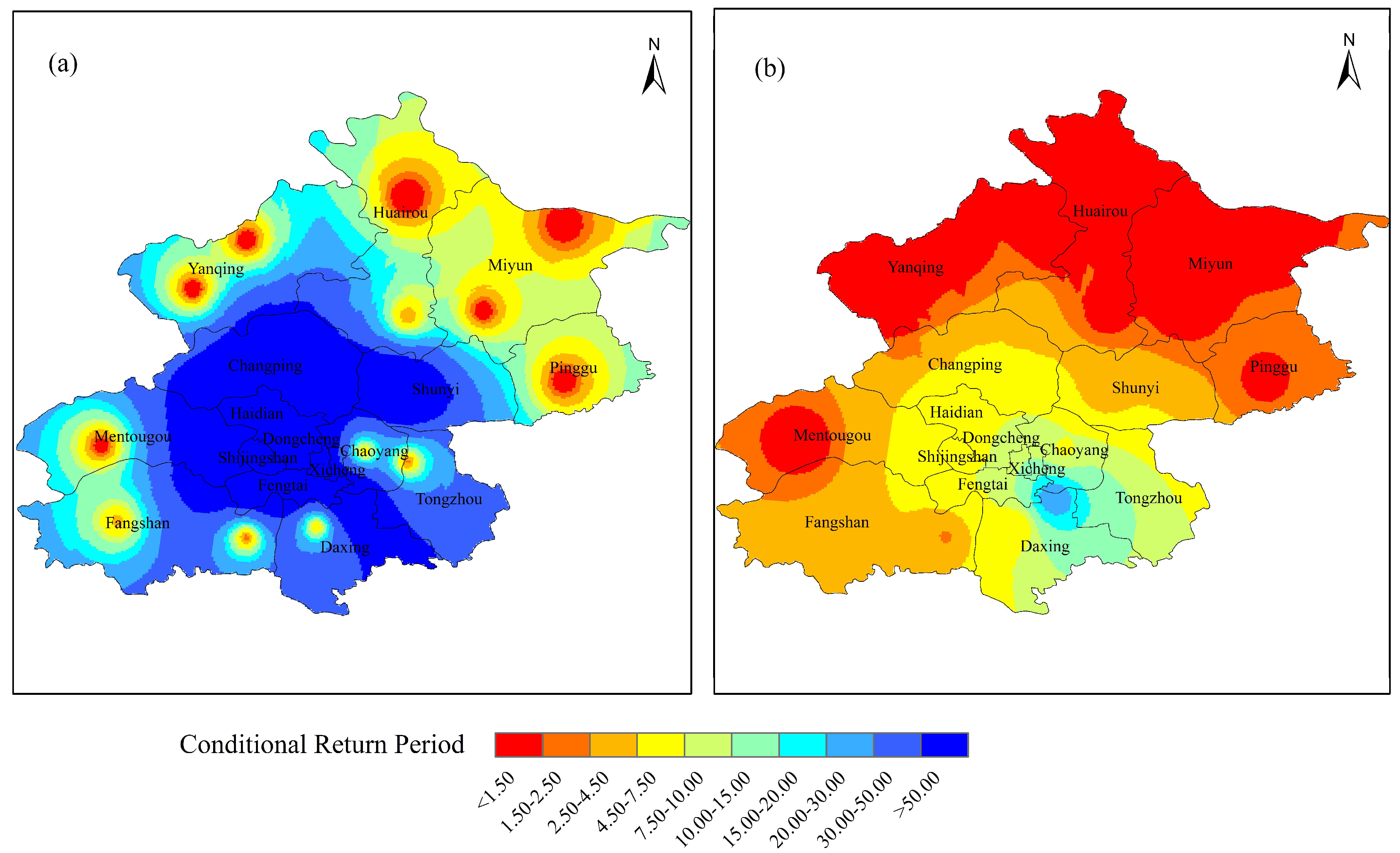
3.2.3. Return Period and Risk Analysis

The return period calculations were supported by IDW interpolation mapping, as shown in Figure 9, Figure 10 and Figure 11. Figure 9 shows the spatial patterns of joint return periods, corresponding to events of duration longer than 2 days and intensity below −15.5 °C. The spatial distributions of the return periods varied between study periods. Short return periods were mainly concentrated in northern and western areas of Beijing, especially in mountainous areas. Long return periods mainly occurred in urban centers. During the period 1978–1998, the return period varied from 0.2 year to almost never. However, during the period 1999–2015, the return period varied from 0.15 to 45 years, showing a general increase in the risk of extreme low temperature events compared with the earlier period. During the period 1978–1998, extreme low temperature events were unlikely in urban centers, while during the period 1999–2015, these centers were likely to experience such an event once every 20 years on average.

The spatial distribution of the conditional return periods corresponding to an intensity below −15.5 °C with a given duration exceeding 2 days is shown in Figure 10. From 1978 to 1998, the return period of $R_{\{T<-15.5|D>2\}}$ varied from 0.1 to 50 years. Short return periods were mainly distributed in northern areas of Beijing, with an average return period of less than 1 year. Meanwhile, southeast areas of Beijing had longer return periods of greater than 10 years. From 1999 to 2015, the return period of $R_{\{T<-15.5|D>2\}}$ varied from 0.1 to 12 years, with an average of 4 years. Short return periods were also mainly distributed in northern areas of Beijing, covering an expanded area compared with the earlier period. The return period in urban centers was less than 10 years, which is much shorter than the return period for the earlier study period. This indicates that events with an intensity below a threshold of −15.5 °C and a given duration exceeding 2 days occurred with increased frequently during the period 1999–2015.

The spatial distributions of conditional return periods of $R_{\{D>2|T<-15.5\}}$ are shown in Figure 11 for both study periods. Clearly, the spatial distribution of the return periods of $R_{\{D>2|T<-15.5\}}$ changed significantly. The return periods from 1978 to 1998 were longer than the return periods for the study period 1999–2015. From 1978 to 1998, extreme low temperature events rarely occurred in most regions of Beijing, although they occurred once every 2 years at Yanqing, Huairou, and Miyun stations. In contrast, the return period varied from 0.15 to 40 years for the study period 1999–2015. Extreme low temperature events were most likely to occur in suburbs, on average every 2 years. The risk of extreme low temperature events was relatively low in all urban areas.

By comparing Figure 10 and Figure 11, it can be found that the conditional return period of $R_{\{T<-15.5|D>2\}}$ is smaller than that of $R_{\{D>2|T<-15.5\}}$. This indicates that the risk of the first scenario corresponding to the conditional return period of $R_{\{T<-15.5|D>2\}}$ (Figure 10) happening is higher than the risk of the second scenario corresponding to the conditional return period of $R_{\{D>2|T<-15.5\}}$ happening (Figure 11), which is different from the comparison between the two conditional return periods for low temperature events.

4. Discussion and Conclusions

Quantifying natural disaster risks using multivariate indicators can lead to an assessment of major natural disasters that is more accurate, and allows preventive measures to be taken earlier to reduce losses of life and property [18,19,20]. In this study, a methodology to establish probabilities and return periods for risk analysis and disaster mitigation using copulas was presented. A risk assessment of two types of winter ECEs in Beijing, namely low temperature and extreme low temperature events, was carried out. An event was described using two variables: duration and intensity. These variables were separately modeled by different marginal distributions and joined using copula functions. Based on the return period function, the joint and conditional return periods were calculated, and their corresponding spatial distributions were discussed.

Six marginal distributions were considered. Generally, the Weibull and GEV distributions provided the best goodness-of-fit for duration and intensity, respectively (Table 4 and Table 7). Three copula functions were applied to construct the bivariate joint probability distribution. The GH copula proved to be the best model for calculating the joint distribution of low temperature event variables (Table 5 and Table 8). Both the GH and Frank copulas were suited to construct the joint distribution of extreme low temperature event variables.

The spatial distributions of different return periods highlighted significant regional differences (Figure 4, Figure 5, Figure 6, Figure 9, Figure 10 and Figure 11). Generally, both low temperature and extreme low temperature events had short joint return periods and conditional return periods in northern and western mountainous areas of Beijing. Events with low temperature and long duration were less likely to occur in urban centers and southeastern areas of Beijing. The spatial distributions of return periods for low temperature and extreme low temperature events were approximately the same, but there were differences in the frequencies of these two kinds of events over the two study periods. These temporal changes suggest that the frequency, duration, and intensity of low temperature events have generally decreased since 1998. In contrast, extreme low temperature events have become longer and more intense in Beijing over the last 18 years, especially in southeastern areas of Beijing, which generally have had a low risk of extreme low temperature events. We found that Beijing experienced fewer events driven by low temperatures, but more events driven by extremely low temperatures over the most recent study period, compared with data from prior to 1998. Such findings support a tendency toward more extreme events as global temperatures rise [35,36,37,38]. Our results provide useful modeling for authorities given that increases in extreme low temperature events will likely become more frequent, despite global warming.

The purpose of this study was to use copula functions to establish a joint probability distribution of meteorological data. Using these distributions, we calculated the joint return period and conditional return period to establish risks related to ECEs. Our results have shown that calculations of the return period based on the copula function can act as an accurate and convenient framework for disaster assessment. Although the study period of 48 years considered herein is relatively short, it demonstrates the advantages of using a joint probability distribution. We plan to extend the time series of ECEs to continue to verify the accuracy of calculated return periods using a larger data set.

References

1. Screen, J.A.; Deser, C.; Sun, L. Reduced risk of North American cold extremes due to continued Arctic sea ice loss. Bull. Am. Meteorol. Soc. 2015, 96, 1489–1503. [Google Scholar] [CrossRef]
2. Cohen, J.; Screen, J.A.; Furtado, J.C.; Barlow, M.; Whittleston, D.; Coumou, D.; Francis, J.; Dethloff, K.; Entekhabi, D.; Overland, J. Recent Arctic amplification and extreme mid-latitude weather. Nat. Geosci. 2014, 7, 627–637. [Google Scholar] [CrossRef] [Green Version]
3. Jennifer, A.; Francis, S.J.V. Evidence linking Arctic amplification to extreme weather in mid-latitudes. Geophys. Res. Lett. 2012, 39, L06801. [Google Scholar]
4. Screen, J.A. Arctic amplification decreases temperature variance in northern mid- to high-latitudes. Nat. Clim. Chang. 2014, 4, 577–582. [Google Scholar] [CrossRef] [Green Version]
5. Zuo, Z.; Zhang, R.; Huang, Y.; Xiao, D.; Guo, D. Extreme cold and warm events over China in wintertime. Int. J. Climatol. 2015, 35, 3568–3581. [Google Scholar] [CrossRef]
6. Jing-Bei, P.; Cholaw, B. The definition and classification of extensive and persistent extreme cold events in China. Atmos. Ocean. Sci. Lett. 2011, 4, 281–286. [Google Scholar] [CrossRef]
7. Wen, M.; Yang, S.; Arun, K.; Zhang, P. An analysis of the large-scale climate anomalies associated with the snowstorms affecting China in January 2008. Mon. Weather Rev. 2009, 137, 1111–1131. [Google Scholar] [CrossRef]
8. Marengo, J.A.; Jones, R.; Alves, L.M.; Valverde, M.C. Future change of temperature and precipitation extremes in South America as derived from the precis regional climate modeling system. Int. J. Climatol. 2010, 29, 2241–2255. [Google Scholar] [CrossRef]
9. Zheng, J.; Ding, L.; Hao, Z.; Ge, Q. Extreme cold winter events in southern China during AD 1650–2000. Boreas 2015, 41, 1–12. [Google Scholar] [CrossRef]
10. Sun, W.; Mu, X.; Song, X.; Wu, D.; Cheng, A.; Qiu, B. Changes in extreme temperature and precipitation events in the loess plateau (China) during 1960–2013 under global warming. Atmos. Res. 2016, 168, 33–48. [Google Scholar] [CrossRef]
11. Choi, G.; Collins, D.; Ren, G.; Trewin, B.; Baldi, M.; Fukuda, Y.; Afzaal, M.; Pianmana, T.; Gomboluudev, P.; Huong, P.T.T.; et al. Changes in means and extreme events of temperature and precipitation in the Asia-Pacific network region, 1955–2007. Int. J. Climatol. 2009, 29, 1906–1925. [Google Scholar] [CrossRef]
12. Cholaw, B.; Xian-Yue, F.U.; Xie, Z.W. Large-scale circulation features typical of wintertime extensive and persistent low temperature events in China. Atmos. Ocean. Sci. Lett. 2011, 4, 235–241. [Google Scholar] [CrossRef]
13. Honda, M.; Inoue, J.; Yamane, S. Influence of low Arctic sea-ice minima on anomalously cold Eurasian winters. Geophys. Res. Lett. 2009, 36, 262–275. [Google Scholar] [CrossRef]
14. Beguería, S. Mapping the hazard of extreme rainfall by peaks-over-threshold extreme value analysis and spatial regression techniques. J. Appl. Meteorol. Climatol. 2006, 45, 108–124. [Google Scholar] [CrossRef]
15. Hanel, M.; Buishand, T.A.; Ferro, C.A.T. A nonstationary index flood model for precipitation extremes in transient regional climate model simulations. J. Geophys. Res. Atmos. 2009, 114, D15107. [Google Scholar] [CrossRef]
16. Krishnamurthy, C.K.B.; Lall, U.; Hyunhan, K. Changing frequency and intensity of rainfall extremes over India from 1951 to 2003. J. Clim. 2009, 22, 4737–4746. [Google Scholar] [CrossRef]
17. Salvadori, G.; Michele, C.D. Frequency analysis via copulas: Theoretical aspects and applications to hydrological events. Water Resour. Res. 2004, 40, 229–244. [Google Scholar] [CrossRef]
18. Rauf, U.F.A.; Zeephongsekul, P. Copula based analysis of rainfall severity and duration: A case study. Theor. Appl. Climatol. 2014, 115, 153–166. [Google Scholar] [CrossRef]
19. Vandenberghe, S.; Verhoest, N.E.C.; Onof, C.; De Baets, B. A comparative copula-based bivariate frequency analysis of observed and simulated storm events: A case study on Bartlett-Lewis modeled rainfall. Water Resour. Res. 2011, 47, 197–203. [Google Scholar] [CrossRef]
20. Singh, V.P.; Zhang, L. Bivariate flood frequency analysis using the copula method. J. Hydrol. Eng. 2006, 11, 150–164. [Google Scholar]
21. Zhang, Y.; Meng, W.; Chen, D.; Guo, W.; Wang, J. The trend of variation for low temperature days over Beijing and its surrounding area. Chin. J. Agrometeorol. 2011, 32, 33–37. (In Chinese) [Google Scholar]
22. Frich, P.; Alexander, L.; Dellamarta, P.; Gleason, B.; Haylock, M.; Klein Tank, A.; Peterson, T. Observed coherent changes in climatic extremes during the second half of the twentieth century. Clim. Res. 2002, 19, 193–212. [Google Scholar] [CrossRef] [Green Version]
23. Kostopoulou, E.; Jones, P.D. Assessment of climate extremes in the Eastern Mediterranean. Meteorol. Atmos. Phys. 2005, 89, 69–85. [Google Scholar] [CrossRef]
24. Russo, S.; Sterl, A. Global changes in indices describing moderate temperature extremes from the daily output of a climate model. J. Geophys. Res. Atmos. 2011, 116, D03104. [Google Scholar] [CrossRef]
25. Frank, J.; Massey, J. The kolmogorov-smirnov test for goodness of fit. J. Am. Stat. Assoc. 1951, 46, 68–78. [Google Scholar]
26. Sklar, M. Fonctions de Répartition À n Dimensions et Leurs Marges; Publications de l’Institut de Statistique de l’Université de Paris: Paris, France, 1959; Volume 8, pp. 229–231. [Google Scholar]
27. Nelsen, R.B. An Introduction to Copulas (Springer Series in Statistics); Springer: New York, NY, USA, 2006; p. 315. [Google Scholar]
28. Zhang, D.D.; Yan, D.H.; Lu, F.; Wang, Y.C.; Feng, J. Copula-based risk assessment of drought in Yunnan province, China. Nat. Hazards 2015, 75, 2199–2220. [Google Scholar] [CrossRef]
29. Kao, S.-C.; Govindaraju, R.S. A bivariate frequency analysis of extreme rainfall with implications for design. J. Geophys. Res. Atmos. 2007, 112, D13119. [Google Scholar] [CrossRef]
30. Joe, H. Multivariate Models and Multivariate Dependence Concepts; Chapman and Hall/CRC: New York, NY, USA, 1997. [Google Scholar]
31. Joe, H. Asymptotic efficiency of the two-stage estimation method for copula-based models. J. Multivar. Anal. 2005, 94, 401–419. [Google Scholar] [CrossRef]
32. Willmott, C.J.; Ackleson, S.G.; Davis, R.E.; Feddema, J.J.; Klink, K.M.; Legates, D.R.; O'Donnell, J.; Rowe, C.M. Statistics for the evaluation and comparison of models. J. Geophys. Res. Oceans 1985, 90, 8995–9005. [Google Scholar] [CrossRef]
33. Shiau, J.T. Return period of bivariate distributed extreme hydrological events. Stoch. Environ. Res. Risk Assess. 2003, 17, 42–57. [Google Scholar] [CrossRef]
34. Watson, D.F. A refinement of inverse distance weighted interpolation. Geo-Processing 1985, 2, 315–327. [Google Scholar]
35. IPCC. Climate Change 2014: Impacts, Adaptation, and Vulnerability. Summaries, Frequently Asked Questions, and Cross-Chapter Boxes. A Contribution of Working Group II to the Fifth Assessment Report of the Intergovernmental Panel on Climate Change; World Meteorological Organization: Geneva, Switzerland, 2014; pp. 81–111. [Google Scholar]
36. Sun, Y.; Zhang, X.; Zwiers, F.W.; Song, L.; Wan, H.; Hu, T.; Yin, H.; Ren, G. Rapid increase in the risk of extreme summer heat in Eastern China. Nat. Clim. Chang. 2014, 4, 1082–1085. [Google Scholar] [CrossRef]
37. Spinoni, J.; Lakatos, M.; Szentimrey, T.; Bihari, Z.; Szalai, S.; Vogt, J.; Antofie, T. Heat and cold waves trends in the carpathian region from 1961 to 2010. Int. J. Climatol. 2015, 35, 4197–4209. [Google Scholar] [CrossRef]
38. Seneviratne, S.I.; Nicholls, N.; Easterling, D.; Goodess, C.M.; Kanae, S.; Kossin, J.; Luo, Y.; Marengo, J.; McInnes, K.; Rahimi, M.; et al. 2012: Changes in climate extremes and their impacts on the natural physical environment. In Managing the Risks of Extreme Events and Disasters to Advance Climate Change Adaptation; Cambridge University Press: Cambridge, UK, 2012; pp. 109–230. [Google Scholar]
Figure 1. The Beijing study area showing the location of the 20 meteorological stations used herein.
Atmosphere 09 00263 g001
Figure 2. Marginal distributions for low temperature event duration (a,c) and intensity (b,d) for Yanqing station for the study periods 1978–1998 (a,b); and 1999–2015 (c,d). EV—extreme value; GEV—generalized EV.
Atmosphere 09 00263 g002
Figure 3. Joint cumulative distributions of intensity and duration for winter low temperature events at Yanqing station for the study periods: (a) 1978–1998, and (b) 1999–2015.
Atmosphere 09 00263 g003
Figure 4. Spatial distributions of joint return periods for low temperature events during study periods: (a) 1978–1998; (b) 1999–2015 (unit: year).
Atmosphere 09 00263 g004
Figure 5. Spatial distributions for the conditional return periods for low temperature events with a duration exceeding 3 days for study periods: (a) 1978–1998; (b) 1999–2015 (unit: year).
Atmosphere 09 00263 g005
Figure 6. Spatial distributions of conditional return periods for low temperature events with a given intensity threshold of below −12 °C and above −15 °C for study periods: (a) 1978–1998; (b) 1999–2015 (unit: year).
Atmosphere 09 00263 g006
Figure 7. Marginal distributions of extreme low temperature event duration (a,c) and intensity (b,d) at Yanqing station for study periods: 1978–1998 (a,b) and 1999–2015 (c,d).
Atmosphere 09 00263 g007
Figure 8. Joint cumulative distributions of intensity and duration of winter extreme low temperature events at Yanqing station for study periods: (a) 1978–1998, (b) 1999–2015.
Atmosphere 09 00263 g008
Figure 9. Spatial distributions of joint return periods for extreme low temperature events the study periods: (a) 1978–1998; (b) 1999–2015 (unit: year).
Atmosphere 09 00263 g009
Figure 10. Spatial distributions of conditional return periods for extreme low temperature events of a given duration exceeding 2 days for study periods: (a) 1978–1998; (b) 1999–2015 (unit: year).
Atmosphere 09 00263 g010
Figure 11. Spatial distributions of conditional return periods for extreme low temperature events with a given intensity threshold of below −15.5 °C for the study periods: (a) 1978–1998; (b) 1999–2015 (unit: year).
Atmosphere 09 00263 g011