Using the Weather Research and Forecasting (WRF) Model for Precipitation Forecasting in an Andean Region with Complex Topography

 ,
,  ,
,
Abstract
:1. Introduction
2. Data and Methods
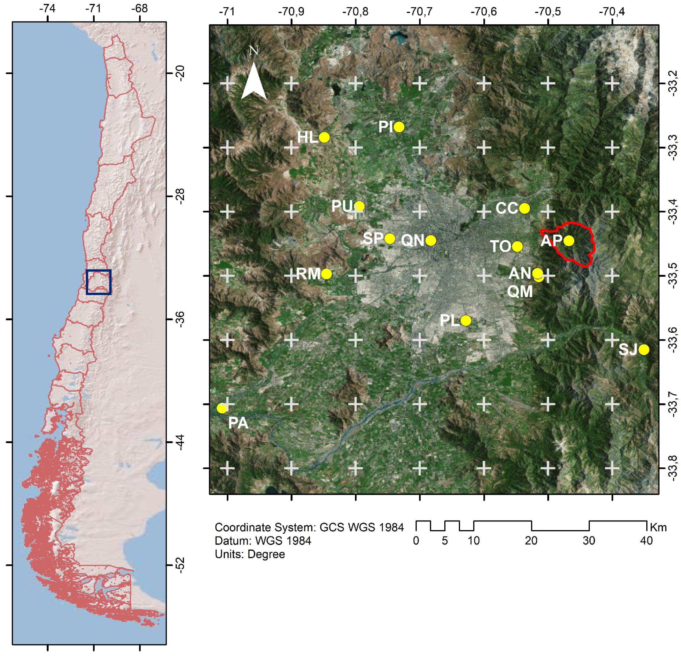
2.1. Field Data
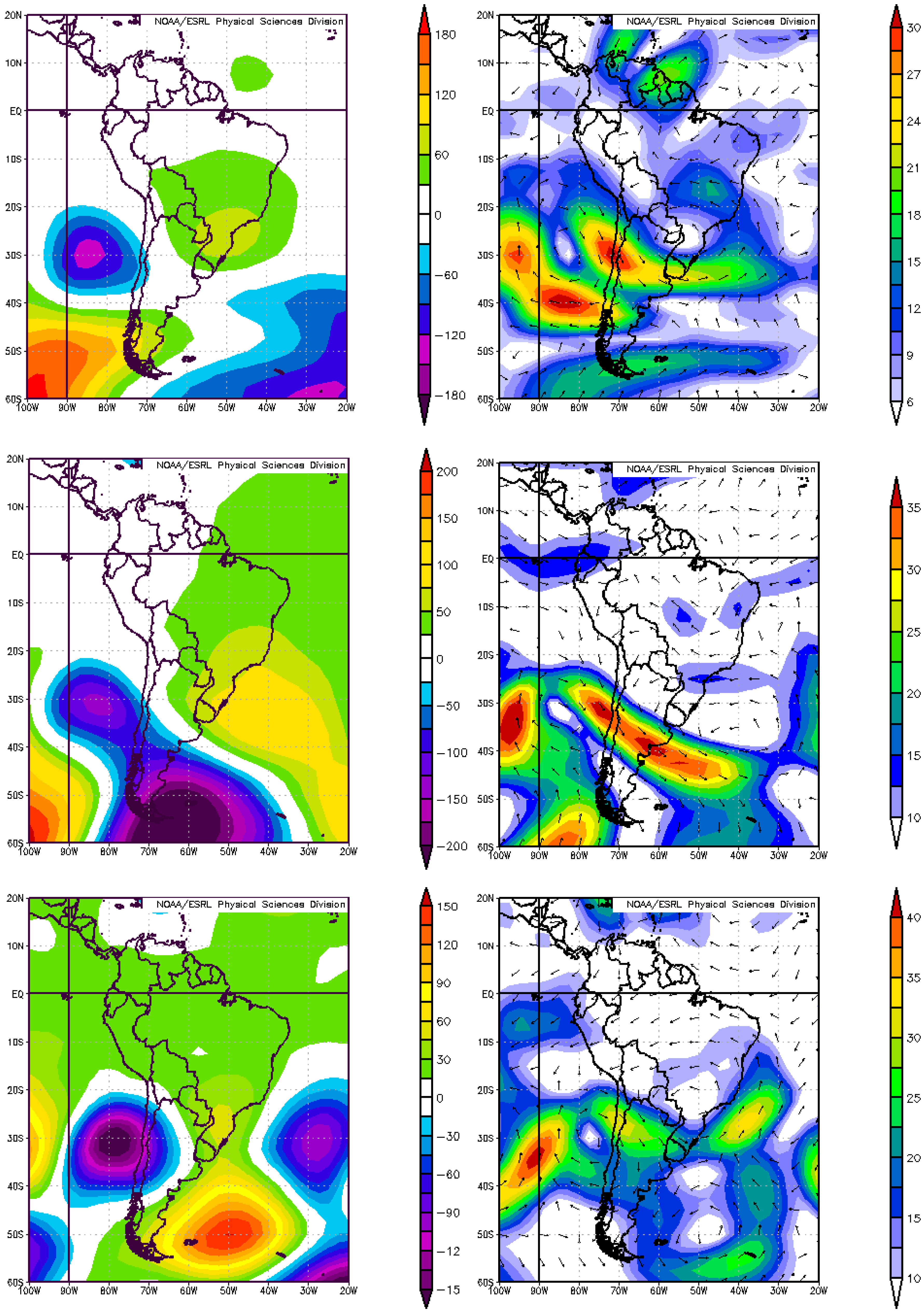
2.2. Meteorological Characterization of Rainfall Events
2.2.1. 19 October 2015 Rainfall Event (OCT15)
2.2.2. 17 April 2016 Rainfall Event (APR16)
2.2.3. 11 May 2017 Rainfall Event (MAY17)
2.3. Meteorological Forcing Data
2.4. WRF Model and Physics Schemes
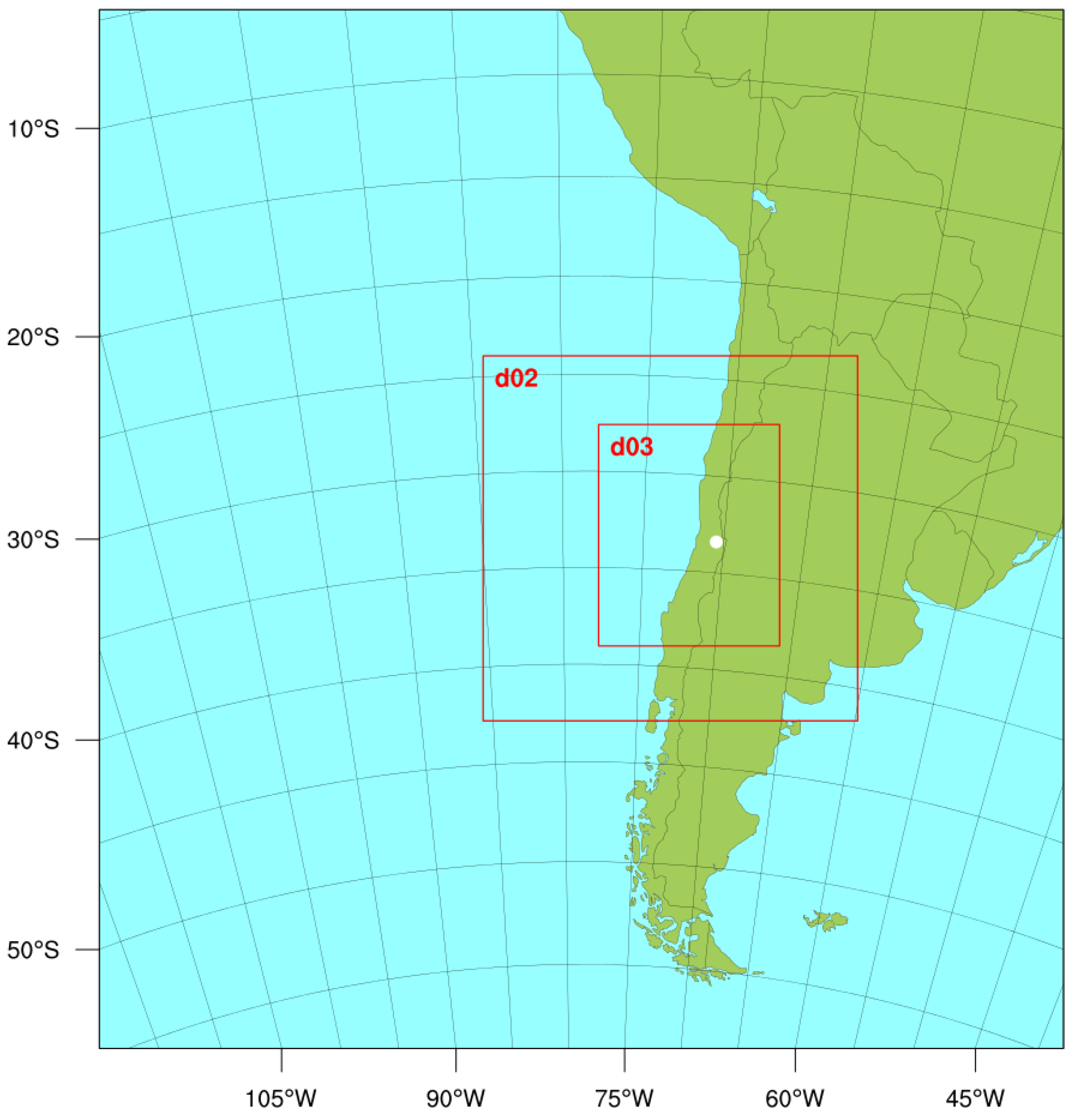
2.4.1. Simulation Domains and Topography Complexity
2.4.2. Physics Schemes and Land Use
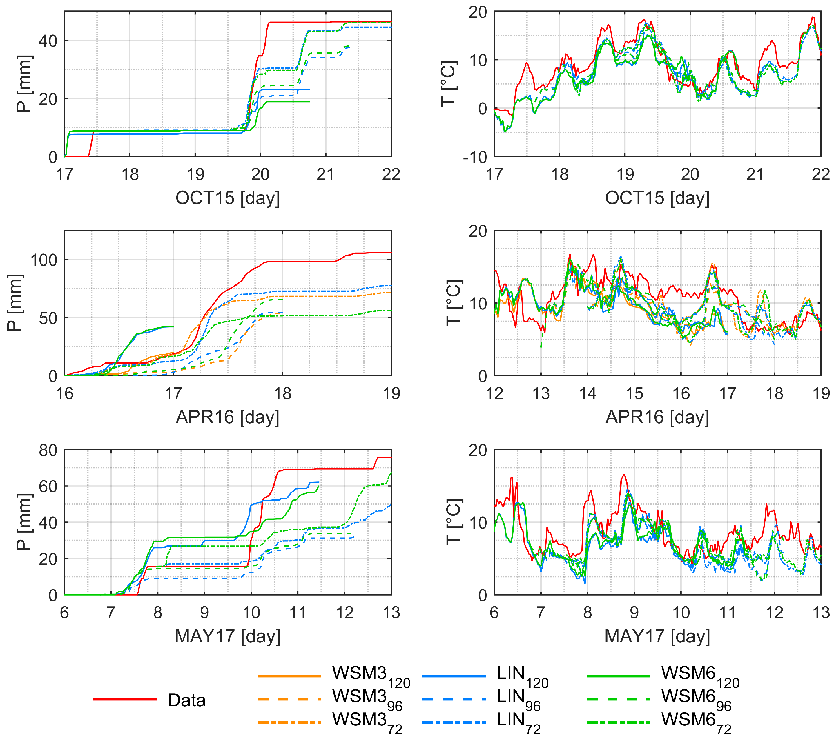
2.4.3. Microphysics
2.4.4. Lead Time
2.5. Model Validation
3. Results
3.1. Local Conditions
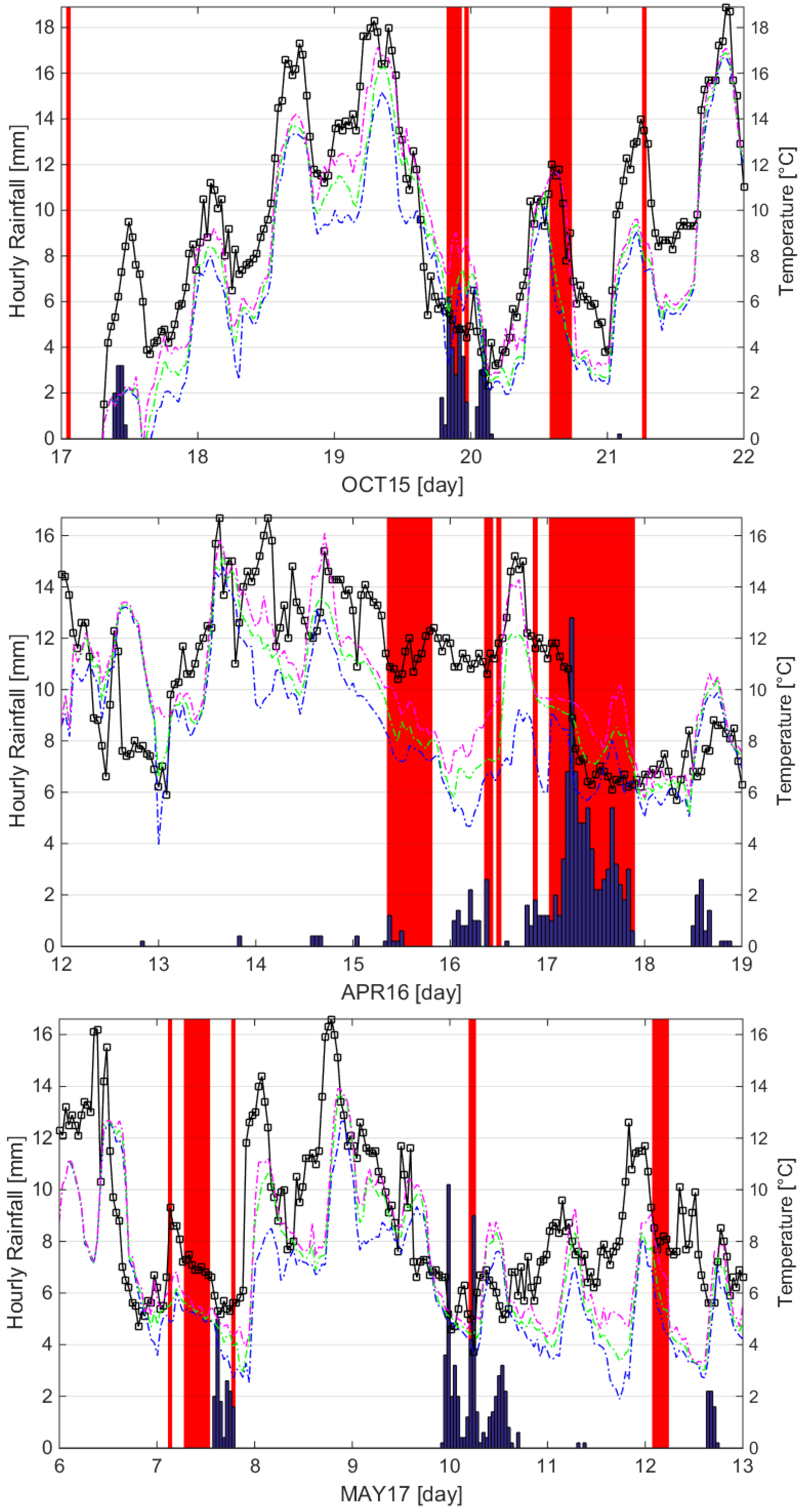
3.2. Rainfall and Temperature Simulation
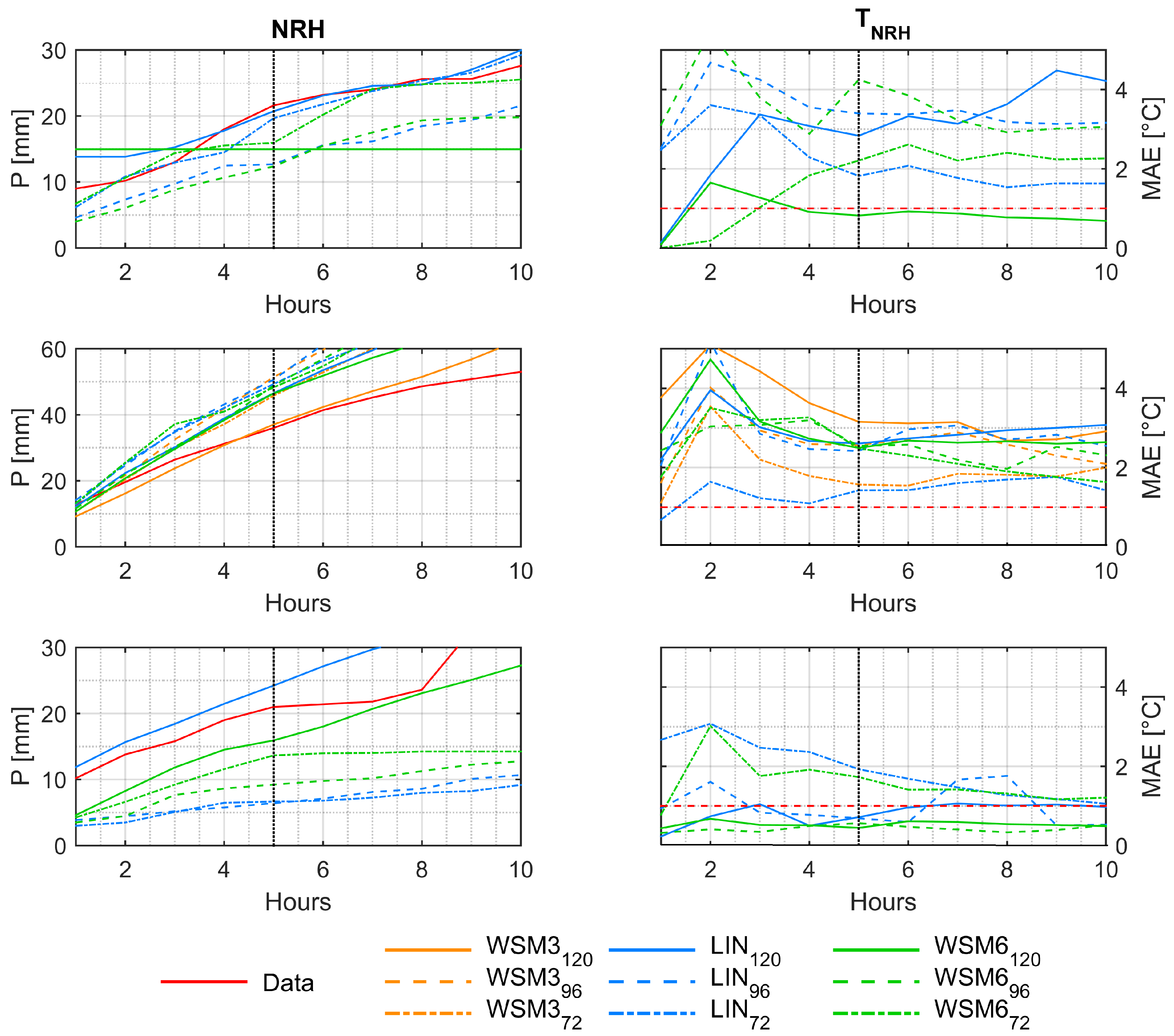
3.3. Rainfall Forecast Performance
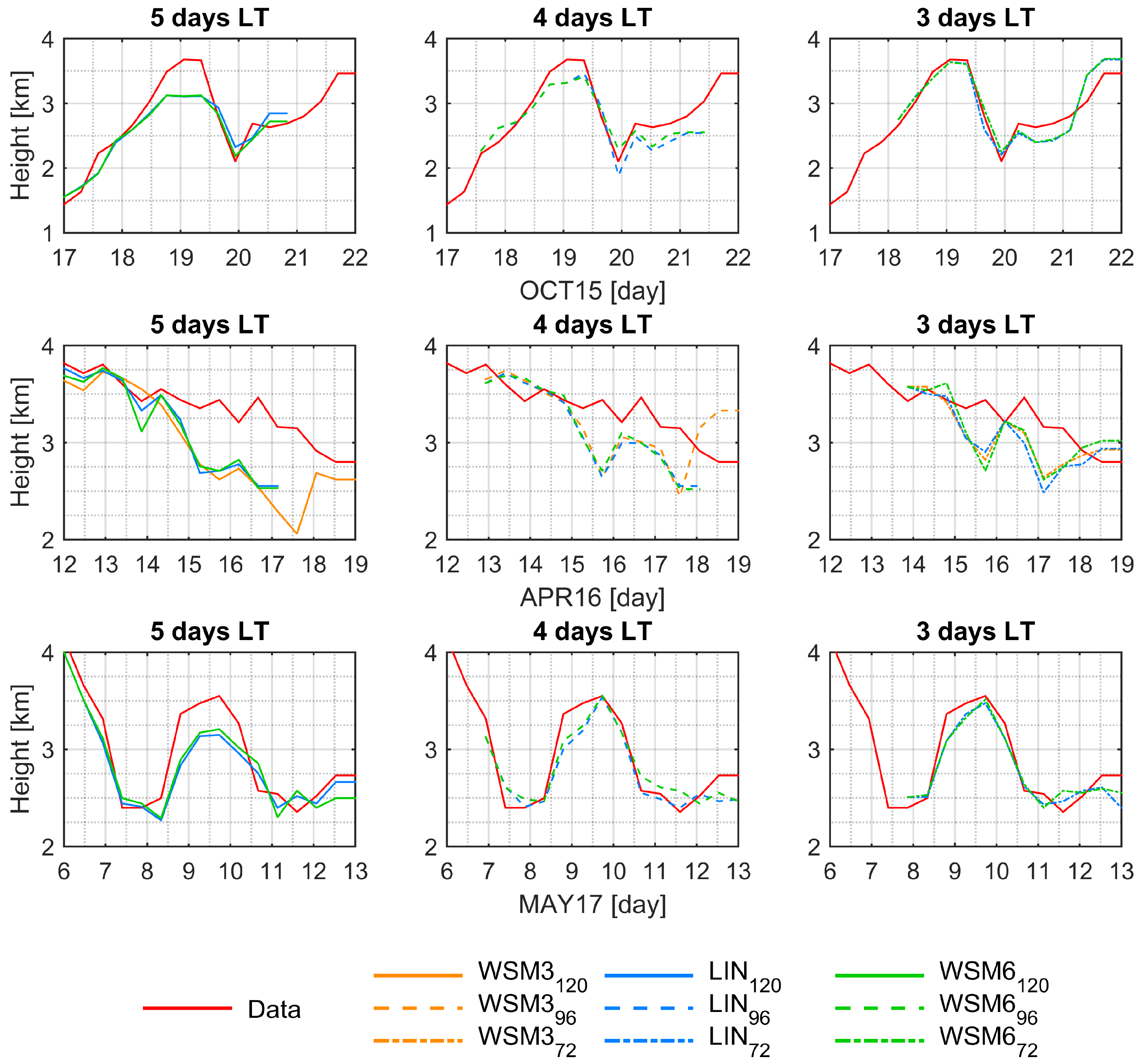
3.4. Freezing Level Height
3.5. Ensemble Performance
4. Conclusions
Author Contributions
Funding
Acknowledgments
Conflicts of Interest
Abbreviations
| ARW | Advanced Research WRF |
| DMC | Chilean Weather Agency |
| FNL | Final Operational Global Analysis data |
| GFS | Global Florecast System |
| LSM | Land Surface Model |
| MODIS | Moderate Resolution Imaging Spectroradiometer |
| MP | Microphysics |
| NCAR | National Center for Atmospheric Research |
| NCEP | National Centers for Environmental Prediction |
| NRH | N-rainiest consecutive hours |
| NWP | Numerical Weather Prediction |
| PBL | Planet Boundary Layer |
| RRTM | Rapid Radiative Transfer Model |
| WRF | Weather Research and Forecasting |
References
- EM-DAT. The International Disaster Database; Technical Report; Centre for Research on the Epidemiology of Disasters (CRED), School of Public Health, Université Catolique de Louvain: Louvain, Bélgica, 2016. [Google Scholar]
- Alfieri, L.; Bisselink, B.; Dottori, F.; Naumann, G.; Roo, A.; Salamon, P.; Wyser, K.; Feyen, L. Global projections of river flood risk in a warmer world. Earth’s Future 2016, 5, 171–182. [Google Scholar] [CrossRef]
- Kundzewicz, Z.W.; Kanae, S.; Seneviratne, S.I.; Handmer, J.; Nicholls, N.; Peduzzi, P.; Mechler, R.; Bouwer, L.M.; Arnell, N.; Mach, K.; et al. Flood risk and climate change: Global and regional perspectives. Hydrol. Sci. J. 2014, 59, 1–28. [Google Scholar] [CrossRef]
- Bozkurt, D.; Rondanelli, R.; Garreaud, R.; Arriagada, A. Impact of warmer Eastern Tropical Pacific SST on the March 2015 Atacama Floods. Mon. Weather Rev. 2016, 144, 4441–4460. [Google Scholar] [CrossRef]
- Wilcox, A.C.; Escauriaza, C.; Agredano, R.; Mignot, E.; Zuazo, V.; Otárola, S.; Castro, L.; Gironás, J.; Cienfuegos, R.; Mao, L. An integrated analysis of the March 2015 Atacama floods. Geophys. Res. Lett. 2016, 43, 8035–8043. [Google Scholar] [CrossRef]
- Directors Guild of America. Caracterización de Suelos y Generación de Información Meteorológica Para Prevención de Riesgos Hidrometeorológicos Cuencas Salado y Copiapó; Technical Report; Dirección General de Aguas—Modelación Ambiental SPA; Directors Guild of America: Sunset Boulevard, CA, USA, 2016. [Google Scholar]
- Otarola, S.; Dimitrova, R.; Leo, L.; Alcafuz, R.; Escauriaza, C.; Arroyo, R.; nez Morroni, G.Y.; Fernando, H.J. On the role of the Andes on weather patterns and related environmental hazards in Chile. In Proceedings of the 19th Joint Conference on the Applications of Air Pollution Meteorology with the AWMA, New Orleans, LA, USA, 10–11 January 2016. [Google Scholar]
- Arnold, D.; Morton, D.; Schicker, I.; Seibert, P.; Rotach, M.W.; Horvarth, K.; Dudhia, J.; Satomura, T.; Muller, M.; Zangl, G.; Takemi, T.; Serafin, S.; Schmidli, J.; Schneider, S. Issues in high-resolution atmospheric modeling in complex topography - The HiRCoT workshop. Croat. Meteorol. J. 2012, 47, 3–11. [Google Scholar]
- Goger, B.; Rotach, M.W.; Gohm, A.; Stiperski, I.; Fuhrer, O. Current challenges for numerical weather prediction in complex terrain: Topography representation and parameterizations. In Proceedings of the 2016 International Conference on High Performance Computing & Simulation (HPCS), Innsbruck, Austria, 18–22 July 2016; pp. 890–894. [Google Scholar] [CrossRef]
- Bongioannini Cerlini, P.; Emanuel, K.A.; Todini, E. Orographic effects on convective precipitation and space-time rainfall variability: Preliminary results. Hydrol. Earth Syst. Sci. 2005, 9, 285–299. [Google Scholar] [CrossRef]
- Houze, R.A. Orographic effects on precipitating clouds. Rev. Geophys. 2012, 50. [Google Scholar] [CrossRef] [Green Version]
- Jiménez, P.A.; Dudhia, J. Improving the representation of resolved and unresolved topographic effects on surface wind in the WRF model. J. Appl. Meteorol. Climatol. 2012, 51, 300–316. [Google Scholar] [CrossRef]
- Lorente-Plazas, R.; Jiménez, P.A.; Dudhia, J.; Montávez, J.P. Evaluating and improving the impact of the atmospheric stability and orography on surface winds in the WRF mode. Mon. Weather Rev. 2016, 144, 2685–2693. [Google Scholar] [CrossRef]
- Madala, S.; Satyanarayana, A.N.V.; Srinivas, C.V.; Boadh, R. Sensitivity of PBL Schemes of WRF-ARW Model in Simulating Mesoscale Atmospheric Flow-Field Parameters Over a Complex Terrain; AGU Fall Meeting Abstracts; American Geophysical Union: Washington, DC, USA, 2014; pp. A43A–3242. [Google Scholar]
- Dimitrova, R.; Silver, Z.; Zsedrovits, T.; Hocut, C.M.; Leo, L.S.; Sabatino, S.D.; Fernando, H.J. Assessment of planetary boundary-layer schemes in the Weather Research and Forecasting mesoscale model using MATERHORN field data. Bound.-Layer Meteorol. 2016, 159, 589–609. [Google Scholar] [CrossRef]
- Siuta, D.; West, G.; Stull, R. WRF hub-height wind forecast sensitivity to PBL scheme, grid length, and initial condition choice in complex terrain. Weather Forecast. 2017, 32, 493–509. [Google Scholar] [CrossRef]
- Pontoppidan, M.; Reuder, J.; Mayer, S.; Kolstad, E.W. Downscaling an intense precipitation event in complex terrain: The importance of high grid resolution. Tellus A Dyn. Meteorol. Oceanogr. 2017, 69, 1271561. [Google Scholar] [CrossRef]
- Mass, C.F.; Ovens, D.; Westrick, K.; Colle, B.A. Does increasing horizontal resolution produce more skillful forecasts? Bull. Am. Meteorol. Soc. 2002, 83, 407–430. [Google Scholar] [CrossRef]
- Gneiting, T.; Raftery, A.E. Weather forecasting with ensemble methods. Science 2005, 310, 248–249. [Google Scholar] [CrossRef] [PubMed]
- Zhang, H.; Pu, Z. Beating the uncertainties: Ensemble forecasting and ensemble-based data assimilation in modern Numerical Weather Prediction. Adv. Meteorol. 2010, 2010, 432160. [Google Scholar] [CrossRef]
- Lee, J.A.; Kolczynski, W.C.; McCandless, T.C.; Haupt, S.E. An objective methodology for configuring and down-selecting an NWP ensemble for low-level wind prediction. Mon. Weather Rev. 2012, 140, 2270–2286. [Google Scholar] [CrossRef]
- Bauer, P.; Thorpe, A.; Brunet, G. The quiet revolution of numerical weather prediction. Nature 2015, 525, 47–55. [Google Scholar] [CrossRef] [PubMed]
- Ruiz, J.J.; Saulo, C.; Nogués-Paegle, J. WRF Model sensitivity to choice of parameterization over South America: Validation against surface variables. Mon. Weather Rev. 2010, 138, 3342–3355. [Google Scholar] [CrossRef]
- Evans, J.P.; Ekström, M.; Ji, F. Evaluating the performance of a WRF physics ensemble over South-East Australia. Clim. Dyn. 2012, 39, 1241–1258. [Google Scholar] [CrossRef]
- Kim, J.H.; Shin, D.B.; Kummerow, C. Impacts of a priori databases using six WRF microphysics schemes on passive microwave rainfall retrievals. J. Atmos. Ocean. Technol. 2013, 30, 2367–2381. [Google Scholar] [CrossRef]
- Katragkou, E.; García-Díez, M.; Vautard, R.; Sobolowski, S.; Zanis, P.; Alexandri, G.; Cardoso, R.M.; Colette, A.; Fernandez, J.; Gobiet, A.; et al. Regional climate hindcast simulations within EURO-CORDEX: Evaluation of a WRF multi-physics ensemble. Geosci. Model Dev. 2015, 8, 603–618. [Google Scholar] [CrossRef] [Green Version]
- Ekström, M. Metrics to identify meaningful downscaling skill in WRF simulations of intense rainfall events. Environ. Model. Softw. 2016, 79, 267–284. [Google Scholar] [CrossRef]
- Hirabayashi, S.; Kroll, C.N.; Nowak, D.J. Component-based development and sensitivity analyses of an air pollutant dry deposition model. Environ. Model. Softw. 2011, 26, 804–816. [Google Scholar] [CrossRef]
- Siddique, R.; Mejia, A.; Brown, J.; Reed, S.; Ahnert, P. Verification of precipitation forecasts from two numerical weather prediction models in the middle Atlantic region of the USA: A precursory analysis to hydrologic forecasting. J. Hydrol. 2015, 529, 1390–1406. [Google Scholar] [CrossRef]
- Buizza, R.; Leutbecher, M. The forecast skill horizon. Q. J. R. Meteorol. Soc. 2015, 141, 3366–3382. [Google Scholar] [CrossRef]
- Skamarock, W.C.; Klemp, J.B.; Dudhia, J.; Gill, D.O.; Barkerand, D.M.; Duda, M.G.; Huang, X.; Wang, W.; Powers, J.G. A Description of the Advanced Research WRF Version 3; NCAR Technical Note; NCAR: Boulder, CO, USA, 2008. [Google Scholar]
- Jiménez, P.A.; González-Rouco, J.F.; García-Bustamante, E.; Navarro, J.; Montávez, J.P.; de Arellano, J.V.G.; Dudhia, J.; Muñoz-Roldan, A. Surface wind regionalization over complex terrain: Evaluation and analysis of a high-resolution WRF simulation. J. Appl. Meteorol. Climatol. 2010, 49, 268–287. [Google Scholar] [CrossRef]
- Zhang, H.; Pu, Z.; Zhang, X. Examination of errors in near-surface temperature and wind from WRF numerical simulations in regions of complex terrain. Weather Forecast. 2013, 28, 893–914. [Google Scholar] [CrossRef]
- Karki, R.; ul Hasson, S.; Gerlitz, L.; Schickhoff, U.; Scholten, T.; Böhner, J. Quantifying the added value of convection-permitting climate simulations in complex terrain: A systematic evaluation of WRF over the Himalayas. Earth Syst. Dyn. 2017, 8, 507–528. [Google Scholar] [CrossRef]
- Soltanzadeh, I.; Bonnardot, V.; Sturman, A.; Quénol, H.; Zawar-Reza, P. Assessment of the ARW-WRF model over complex terrain: The case of the Stellenbosch Wine of Origin district of South Africa. Theor. Appl. Climatol. 2017, 129, 1407–1427. [Google Scholar] [CrossRef]
- Jiménez-Esteve, B.; Udina, M.; Soler, M.; Pepin, N.; Miró, J. Land use and topography influence in a complex terrain area: A high resolution mesoscale modelling study over the Eastern Pyrenees using the WRF model. Atmos. Res. 2018, 202, 49–62. [Google Scholar] [CrossRef]
- Garreaud, R.; Falvey, M.; Montecinos, A. Orographic precipitation in coastal southern Chile: Mean distribution, temporal variability, and linear contribution. J. Hydrometeorol. 2016, 17, 1185–1202. [Google Scholar] [CrossRef]
- Puliafito, S.; Allende, D.; Mulena, C.; Cremades, P.; Lakkis, S. Evaluation of the WRF model configuration for Zonda wind events in a complex terrain. Atmos. Environ. 2015, 166, 24–32. [Google Scholar] [CrossRef]
- Saide, P.E.; Carmichael, G.R.; Spak, S.N.; Gallardo, L.; Osses, A.E.; Mena-Carrasco, M.A.; Pagowski, M. Forecasting urban PM10 and PM2.5 pollution episodes in very stable nocturnal conditions and complex terrain using WRF-Chem CO tracer model. Atmos. Environ. 2011, 45, 2769–2780. [Google Scholar] [CrossRef]
- Catalán, M. Acodicionamiento de un Modelo Hidrológico Geomorfológico Urbano de Onda Cinemática para su Aplicación en Cuencas Naturales. Ph.D. Thesis, Pontificia Universidad Católica de Chile, Santiago, Chile, 2013. [Google Scholar]
- Garreaud, R.; Rutllant, J. Precipitación estival en los Andes de Chile central: Aspectos climatológicos. Atmósfera 1997, 10, 191–211. [Google Scholar]
- Vargas, X. Corrientes de detritos en la Quebrada de Macul, Chile. Estudio de caudales máximos. Ingeniería del Agua 1999, 6, 341–344. [Google Scholar] [CrossRef]
- Dirección General de Aeronáutica Civil (DGAC). Dirección Meteorológica de Chile (DMC). Available online: http://www.meteochile.cl (accessed on 22 March 2018).
- Mann, H.B. Nonparametric tests against trend. Econometrica 1945, 13, 245–259. [Google Scholar] [CrossRef]
- Kendall, M.G. Rank Correlation Methods, 4th ed.; Griffin, Charles: London, UK, 1975; p. 272. [Google Scholar]
- Garreaud, R.D.; Alvarez-Garreton, C.; Barichivich, J.; Boisier, J.P.; Christie, D.; Galleguillos, M.; LeQuesne, C.; McPhee, J.; Zambrano-Bigiarini, M. The 2010–2015 megadrought in central Chile: Impacts on regional hydroclimate and vegetation. Hydrol. Earth Syst. Sci. 2017, 21, 6307–6327. [Google Scholar] [CrossRef]
- University of Wyoming. College of Engineering. Soundings. Available online: http://weather.uwyo.edu/upperair/sounding.html (accessed on 22 March 2018).
- Roney, J.A. Statistical wind analysis for near-space applications. J. Atmos. Sol.-Terr. Phys. 2007, 69, 1485–1501. [Google Scholar] [CrossRef]
- Fuenzalida, H.; Sanchez, R.; Garreaud, R. A climatology of cutoff lows in the Southern Hemisphere. J. Geophys. Res. Atmos. 2005, 110. [Google Scholar] [CrossRef] [Green Version]
- Garreaud, R.; Fuenzalida, H. The Influence of the Andes on Cutoff Lows: A Modeling Study. Mon. Weather Rev. 2007, 135, 1596–1613. [Google Scholar] [CrossRef]
- Aguilar, X. Análisis de Eventos Extremos de Precipitación en División Los Bronces, Cordillera Central de Chile. Ph.D. Thesis, Tesis Para Optar al Título Profesional de Meteorólogo, Departamento de Meteorología, Universidad de Valparaíso, Valparaíso, Chile, 2010. [Google Scholar]
- MOP. Manual de Drenaje Urbano: Guía para el Diseño, Construcción, Operación y Conservación de Obras de Drenaje Urbano; Technical Report; Ministerio de Obras Públicas: Santiago, Chile, 2013. [Google Scholar]
- Garreaud, R. Warm winter storms in central Chile. J. Hydrometeorol. 2013, 14, 1515–1534. [Google Scholar] [CrossRef]
- National Center for Atmospheric Research (NCAR). WRF Users Page. Available online: http://www.mmm.ucar.edu/wrf/users (accessed on 22 March 2018).
- National Oceanic and Atmospheric Administration (NOAA). National Centers for Environmental Information. ModelData. Available online: https://www.ncdc.noaa.gov/data-access/model-data/ (accessed on 22 March 2018).
- National Centers for Environmental Prediction (NCEP). NCEP FNL Operational Model Global Tropospheric Analyses, Continuing from July 1999. Available online: http://rda.ucar.edu/datasets/ds083.2/ (accessed on 22 March 2018).
- Carvalho, D.; Rocha, A.; Gomez-Gesteira, M.; Santos, C. A sensitivity study of the WRF model in wind simulation for an area of high wind energy. Environ. Model. Softw. 2012, 33, 23–34. [Google Scholar] [CrossRef] [Green Version]
- Aligo, E.A.; Gallus, W.A.; Segal, M. On the impact of WRF model vertical grid resolution on midwest summer rainfall forecasts. Weather Forecast. 2009, 24, 575–594. [Google Scholar] [CrossRef]
- Seaman, N.; Gaudet, B.; Zielonka, J.; Stauffer, D. Sensitivity of vertical structure in the stable boundary layer to variations of the WRF model’s Mellor Yamada Janjic turbulence scheme. In Proceedings of the 9th WRF Users Workshop, Boulder, CO, USA, 23–27 June 2008. [Google Scholar]
- Rahn, D.A.; Garreaud, R. Marine boundary layer over the subtropical southeast Pacific during VOCALS-REx. Part 1: Mean structure and diurnal cycle. Atmos. Chem. Phys. 2010, 10, 4491–4506. [Google Scholar] [CrossRef]
- Dudhia, J. Numerical study of convection observed during the winter monsoon experiment using a mesoscale two-dimensional model. J. Atmos. Sci. 1989, 46, 3077–3107. [Google Scholar] [CrossRef]
- Mlawer, E.J.; Taubman, S.J.; Brown, P.; Iacono, M.J.; Clough, S.A. Radiative transfer for inhomogeneous atmospheres: RRTM, a validated correlated-k model for the longwave. J. Geophys. Res. Atmos. 1997, 102, 16663–16682. [Google Scholar] [CrossRef] [Green Version]
- Grell, G.A. Prognostic evaluation of assumptions used by cumulus parameterizations. Mon. Weather Rev. 1993, 121, 746–787. [Google Scholar] [CrossRef]
- Niu, G.Y.; Yang, Z.L.; Mitchell, K.E.; Chen, F.; Ek, M.B.; Barlage, M.; Kumar, A.; Manning, K.; Niyogi, D.; Rosero, E.; et al. The community Noah land surface model with multiparameterization options (Noah-MP): 1. Model description and evaluation with local-scale measurements. J. Geophys. Res. Atmos. 2011, 116, n/a. [Google Scholar] [CrossRef]
- Nakanishi, M.; Niino, H. An improved Mellor–Yamada level-3 model: Its numerical stability and application to a regional prediction of advecting fog. Bound.-Layer Meteorol. 2006, 119, 397–407. [Google Scholar] [CrossRef]
- Liu, C.; Ikeda, K.; Thompson, G.; Rasmussen, R.; Dudhia, J. High-Resolution Simulations of Wintertime Precipitation in the Colorado Headwaters Region: Sensitivity to Physics Parameterizations. Mon. Weather Rev. 2011, 139, 3533–3553. [Google Scholar] [CrossRef]
- Lin, T.; Farley, R.D.; Orville, H.D. Bulk parameterization of the snow field in a cloud model. J. Clim. Appl. Meteorol. 1983, 22, 1065–1092. [Google Scholar] [CrossRef]
- Hong, S.Y.; Lim, J.O.J. The WRF single-moment 6-class microphysics scheme (WSM6). J. Korean Meteor. Soc. 2006, 42, 129–151. [Google Scholar]
- Caneo, M. Sensibilidad a Diferentes Esquemas De Microfísica del WRF, en Chajnator-Chile. Ph.D. Thesis, Tesis Para Optar al Título Profesional de Meteorólogo, Departamento de Meteorología, Universidad de Valparaíso, Valparaíso, Chile, 2010. [Google Scholar]
- Sikder, S.; Hossain, F. Assessment of the weather research and forecasting model generalized parameterization schemes for advancement of precipitation forecasting in monsoon-driven river basins. J. Adv. Model. Earth Syst. 2016, 8, 1210–1228. [Google Scholar] [CrossRef] [Green Version]
- Willmott, C.J.; Robeson, S.M.; Matsuura, K. A refined index of model performance. Int. J. Climatol. 2012, 32, 2088–2094. [Google Scholar] [CrossRef]
- Zegpi, M.; Fernández, B. Hydrological model for urban catchments—Analytical development using copulas and numerical solution. Hydrol. Sci. J. 2010, 55, 1123–1136. [Google Scholar] [CrossRef]
- Thompson, G.; Field, P.R.; Rasmussen, R.M.; Hall, W.D. Explicit forecasts of winter precipitation using an improved bulk microphysics scheme. Part II: Implementation of a new snow parameterization. Mon. Weather Rev. 2008, 136, 5095–5115. [Google Scholar] [CrossRef]
- Thompson, G.; Eidhammer, T. A study of aerosol impacts on clouds and precipitation development in a large winter cyclone. J. Atmos. Sci. 2014, 71, 3636–3658. [Google Scholar] [CrossRef]
- Caseri, A.; Ramos, M.; Javelle, P.; Leblois, E. A space-time geostatistical approach for ensemble rainfall nowcasting. In Proceedings of the 3rd European Conference on Flood Risk Management, Lyon, France, 17–21 October 2016. [Google Scholar] [CrossRef]
- Kumari, M.; Singh, C.K.; Bakimchandra, O.; Basistha, A. DEM-based delineation for improving geostatistical interpolation of rainfall in mountainous region of Central Himalayas, India. Theor. Appl. Climatol. 2017, 130, 51–58. [Google Scholar] [CrossRef]
- Kumari, M.; Singh, C.K.; Basistha, A. Clustering Data and Incorporating Topographical Variables for Improving Spatial Interpolation of Rainfall in Mountainous Region. Water Resour. Manag. 2017, 31, 425–442. [Google Scholar] [CrossRef]


| Name | ID | Latitude | Longitude | Elevation (m.a.s.l.) | Variables |
|---|---|---|---|---|---|
| San José Guayacán | SJ | S | W | 928 | Hourly T, P |
| Apoquindo | AP | S | W | 1625 | Hourly T, P |
| Quebrada de Macul * | QM | S | W | 950 | Daily T, P |
| Antupirén * | AN | S | W | 904 | Daily P |
| Cerro Calán * | CC | S | W | 904 | Daily T, P |
| Tobalaba * | TO | S | W | 650 | Daily T, P |
| La Platina * | PL | S | W | 630 | Hourly T, P |
| Quinta Normal * | QN | S | W | 534 | Daily T, P |
| Lo Pinto * | PI | S | W | 512 | Hourly T, P |
| San Pablo * | SP | S | W | 490 | Hourly T, P |
| Pudahuel | PU | S | W | 482 | Daily T, P |
| Rinconada de Maipú | RM | S | W | 462 | Hourly T, P |
| Hacienda Lampa | HL | S | W | 493 | Hourly T, P |
| El Paico | PA | S | W | 275 | Hourly T, P |
| Physical Scheme | Parametrization |
|---|---|
| Short-wave radiation | Dudhia |
| Long-wave radiation | RRTM |
| Cumulus | Grell 3D Ensemble |
| Planet Boundary Layer | MMYN |
| Soil Layer | MMYN |
| Land Surface Model | Noah-MP |
| Rainfall Event | MP Schemes | Simulation Beginning (00:00) | Lead Times (h) | Simulations |
|---|---|---|---|---|
| OCT15 | LIN & WSM6 | 15, 16 & 17 October 2015 | 72, 96 & 120 | 6 |
| APR16 | LIN, WSM3 & WSM6 | 12, 13 & 14 April 2016 | 72, 96 & 120 | 9 |
| MAY17 | LIN & WSM6 | 6, 7 & 8 May 2017 | 72, 96 & 120 | 6 |
| Meteorological Variable | Absolute Difference Tolerance Criteria |
|---|---|
| Dew temperature | 1 °C in surface, 2 °C in atmosphere |
| Temperature | 1 °C in surface, 2 °C in atmosphere |
| Wind speed | 2.57 m/s (∼5 knots) for all data |
| Wind direction | 20 in surface, 15 in pressure levels above the 850 hPa |
© 2018 by the authors. Licensee MDPI, Basel, Switzerland. This article is an open access article distributed under the terms and conditions of the Creative Commons Attribution (CC BY) license (http://creativecommons.org/licenses/by/4.0/).
Share and Cite
Yáñez-Morroni, G.; Gironás, J.; Caneo, M.; Delgado, R.; Garreaud, R. Using the Weather Research and Forecasting (WRF) Model for Precipitation Forecasting in an Andean Region with Complex Topography. Atmosphere 2018, 9, 304. https://doi.org/10.3390/atmos9080304
Yáñez-Morroni G, Gironás J, Caneo M, Delgado R, Garreaud R. Using the Weather Research and Forecasting (WRF) Model for Precipitation Forecasting in an Andean Region with Complex Topography. Atmosphere. 2018; 9(8):304. https://doi.org/10.3390/atmos9080304
Chicago/Turabian StyleYáñez-Morroni, Gonzalo, Jorge Gironás, Marta Caneo, Rodrigo Delgado, and René Garreaud. 2018. "Using the Weather Research and Forecasting (WRF) Model for Precipitation Forecasting in an Andean Region with Complex Topography" Atmosphere 9, no. 8: 304. https://doi.org/10.3390/atmos9080304