Numerical Simulation of a Heavy Precipitation Event in the Vicinity of Madrid-Barajas International Airport: Sensitivity to Initial Conditions, Domain Resolution, and Microphysics Parameterizations

Abstract

Deep convection is a threat to many human activities, with a great impact on aviation safety. On 7 July 2017, a widespread torrential precipitation event (associated with a cut-off low at mid-levels) was registered in the vicinity of Madrid, causing serious flight disruptions. During this type of episode, accurate short-term forecasts are key to minimizing risks to aviation. The aim of this research is to improve early warning systems by obtaining the best WRF model setup. In this paper, the aforementioned event was simulated. Various model configurations were produced using four different physics parameterizations, 3-km and 1-km domain resolutions, and 0.25° and 1° initial condition resolutions. Simulations were validated using data from 17 rain gauge stations. Two validation indices are proposed, accounting for the temporal behaviour of the model. Results show significant differences between microphysics parameterizations. Validation of domain resolution shows that improvement from 3 to 1 km is negligible. Interestingly, the 0.25° resolution for initial conditions produced poor results compared with 1°. This may be linked to a timing error, because precipitation was simulated further east than observed. The use of ensembles generated by combining different WRF model configurations produced reliable precipitation estimates.

1. Introduction

Heavy precipitation poses a significant risk to human activities in several parts of the world [1]. Meteorological phenomena related to deep convection cause thousands of casualties and huge economic losses worldwide every year [2]. The main risks associated with this type of atmospheric phenomena are heavy precipitation, gale-force wind gusts, hail, and lightning [3,4]. In particular, the Iberian Peninsula is a region favourable for the development of deep convection systems during the warm season [5]. Some heavy precipitation events of the Iberian Peninsula have been analysed because of their associated hazards and risks [6].

Early warning systems may decrease the damage caused by deep convection, and are mainly based on an accurate weather forecast [7]. Nevertheless, the forecasting of heavy precipitation episodes is still a challenge for numerical weather prediction models [8]. The reason is linked to the fact that these events are strongly affected by mesoscale processes (such as convection and radiation) that must be parameterized by numerical models [9]. These parameterizations are case-dependent, so it is convenient to consider the use of an ensemble composed of different physical parameterizations [10].

When evaluating model performance, precipitation is an interesting field because it is unlikely to easily achieve accurate verification [11]. Risky situations caused by heavy precipitation are not only related to large amounts of accumulated precipitation (that can be obtained by persistent precipitation over long periods) but also to strong precipitation intensities over a few hours [12]. Therefore, different validation methods must be used to evaluate both accumulated precipitation and the temporal evolution of precipitation rate. Both mean absolute error (MAE) and root mean square error (RMSE) are adequate for testing the accumulated precipitation estimated by a numerical weather prediction model, by comparing it to precipitation measured in a region during a specific period [13]. Nevertheless, these validation indices do not provide information about the accuracy of the temporal evolution of precipitation. As a result, good verification scores can be obtained in spite of modelled precipitation being forecast in a different time interval than the observed precipitation. In this regard, the Pearson’s correlation coefficient is commonly used for the evaluation of the similarity of precipitation temporal evolution between forecast and observed precipitation time series [14]. However, strong correlation can be obtained when modelled and observed precipitation maxima are acquired at the same time, despite their magnitudes (and consequently accumulated precipitation) being very distinct. Therefore, it seems most appropriate to evaluate both total accumulated precipitation and temporal evolution of the precipitation rate together, using indices that integrate both types of validation.

This paper analyses a deep convection episode at the centre of the Iberian Peninsula on 7 July 2017, causing widespread heavy precipitation. This event was linked to a cut-off low at mid-levels over the southwestern part of that peninsula. This low was originated by an extratropical cyclone in the North Atlantic that was isolated from the general circulation of the atmosphere (characterized by westerlies at those latitudes), forming a closed cyclonically circulating eddy in the middle and upper troposphere, where the air is colder than the surroundings. In addition, warm temperatures on the surface and at low levels of the troposphere caused strong instability, generating ideal conditions for the development of deep convection. As a result, dozens of flights were diverted or cancelled at the Adolfo Suárez Madrid-Barajas International Airport (LEMD hereafter, per the airport’s International Civil Aviation Organization code). In addition, there were dramatic traffic jams on the main highways of Madrid.

With the aim of improving the forecast of future heavy precipitation episodes, the aforementioned event was simulated by the weather research and forecasting (WRF) model. Several initial conditions, model resolutions, and physics parameterizations were tested to discover which setup was optimal for forecasting this type of episode in the study area. Accumulated precipitation was not only analysed, but also the temporal evolution and geographic distribution of precipitation, by comparing the precipitation rate estimated by the model and observed values from multiple weather stations within the study area. Thus, two validation indices are proposed, which take into account both accumulated precipitation and its temporal evolution.

The paper is organized as follows. The experimental design is detailed in Section 2, including a description of the study area, the model setup, and information about observational data. Section 3 explains the main results of this investigation, followed by Section 4, in which results and an integrating discussion are presented.

2. Experiment

2.1. Area of Study

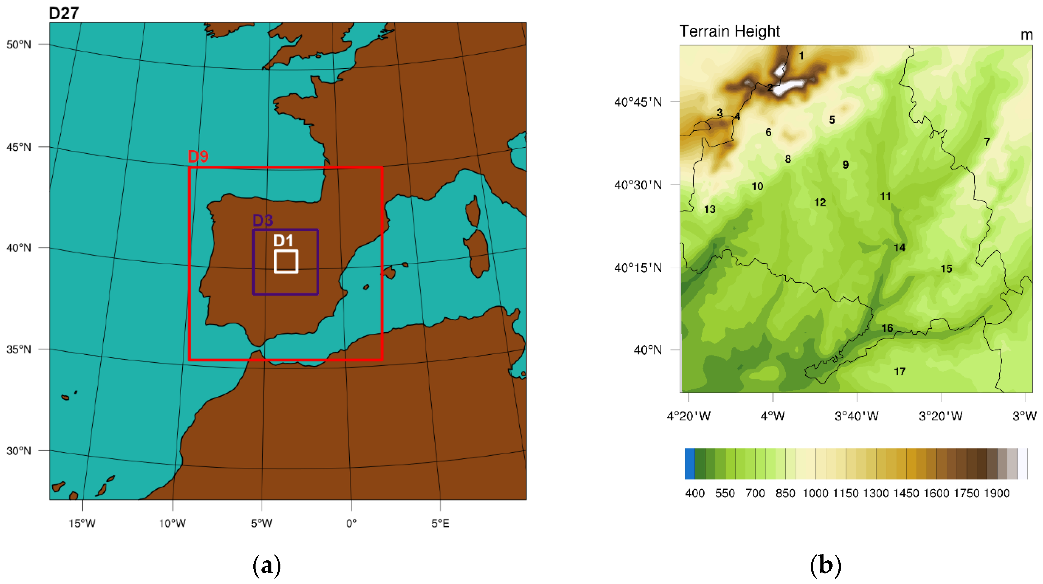
This work focused on the area close to LEMD. The airport is near the centre of the Iberian Peninsula, a few kilometres northeast of the city of Madrid at an elevation of 609 m above sea level (m.a.s.l.). The main orographic feature in the surrounding area is the Guadarrama mountain range (within the Central System), which runs in a southwest-northeast direction approximately 50 km northwest of the airport, with elevations higher than 2300 m.a.s.l. (Figure 1b). To the southeast of this range, a small plateau extends up to the Tajo Valley, which runs from east to west approximately 50 km south of the airport, with elevations lower than 500 m.a.s.l. The climatology of the airport in July is marked by two predominant wind directions, north and southwest, both with similar frequencies, but the southwesterlies are more intense [15]. Owing to the terrain configuration, orographic blocking protects the area from precipitation during northerly winds, but enhances precipitation during southerly winds. The mean maximum temperature in July is 33.5 °C, and the mean minimum is 16.8 °C. Mean monthly precipitation is 9 mm for the month [15]. On the day of the event, 44.7 mm was measured at the airport.

The LEMD is the busiest airport in Spain, with more than daily 1000 operations (take-offs and landings). It is one of the major gateways of air traffic into Europe and ranks among the 50 busiest airports in the world. With regard to aviation safety, heavy precipitation events generate reduced visibility, contaminated runways, reduced braking action, and reduced aerodynamic performance of aircraft. Sudden and strong precipitation can result in substantial disruption of airport operation, affecting arriving and departing aircraft many hours after the precipitation has disappeared.

2.2. Model Configuration

The experiment consisted of several numerical simulations of the studied event and their validation against observational data. The simulations were performed with the advanced research WRF model version 3.7.1. This is a non-hydrostatic model with several parameterization options, which has been extensively proven and validated for weather prediction and research [16]. All simulations were conducted from 00:00 to 24:00 UTC, 7 July 2017. Initial and boundary conditions were taken from the Global Forecast System (GFS) reanalysis developed by the National Centers for Environmental Prediction (NCEP). It was decided to use this database because of free access. Grid resolutions 1° × 1° and 0.25° × 0.25° were used (GFS1 and GFS025 hereafter), providing data at 6 and 3 h intervals, respectively. For GFS1, WRF was configured in 4 domains, 120 × 120 grid points each, with 27, 9, 3, and 1 km grid resolutions (D27, D9, D3, and D1 hereafter). All domains were approximately centred on LEMD (Figure 1a). Only D9, D3, and D1 were used for GFS025. This time and domain configuration was chosen to allow for spin-up time (validation began at 10:00 UTC) but minimizing lead time to the event, and to use relatively small outer domains. Both conditions have been proven to perform better statistically with long lead times and large outer domains [17].

A two-way nesting strategy was chosen. Sixty sigma levels were defined with a progressive resolution, greater in the lower levels of the troposphere. All other parameters not mentioned were identical for every simulation.

Model results were produced every hour for D3 and every 10 min for D1. For standardization and validation comparison, only hourly results were considered for D1. For grid point data, the closest grid point to the geographic location was used for D3. For D1 results, an average value was determined from data in a 3 × 3 grid from the nearest grid point. Thus, the validated areas in D1 and D3 are equivalent and the results of validation are comparable.

2.3. Physics Parameterizations

The simulated precipitation during deep convection episodes depends mainly on microphysics schemes used in the model [8,17,18]. In this experiment, we assessed the sensitivity of the model to three microphysics parameterizations:

• Thompson scheme [19]: This is a single-moment scheme but adds a double moment (mass of hydrometeors and number concentration are independently predicted) for rain and cloud ice. It determines the hydrometeor mixing ratio and the number concentration for rain and cloud ice. Snow size was controlled by ice water content and temperature. Snow shape was non-spherical and density varied inversely with diameter. It considered six types of hydrometeors: water vapour, cloud water, rain water, cloud ice, snow, and graupel.
• Milbrandt–Yau scheme [20,21]: This is a double-moment scheme (although it allows up to three moments). Mixing ratio and number concentration was predicted for cloud and hydrometeors. Radar reflectivity as predicted for some hydrometeors. It considered seven types of hydrometeors: water vapour, cloud water, rain water, cloud ice, snow, graupel, and hail.
• Morrison scheme [22]: This is a double-moment scheme that includes predicted mixing ratios and number concentrations for cloud water, cloud ice, rain, and snow. It also includes a predicted rain size distribution and different rates of rain evaporation for convective and stratiform clouds. It considered six types of hydrometeors: water vapour, cloud water, rainwater, cloud ice, snow, and graupel.

For these three microphysics schemes, the same physics parameterizations are used: New Goddard as long and short wave radiation schemes [23], Unified Noah as the surface scheme [24], Eta Similarity as the clay scheme [25], and Mellor–Yamada–Janjic (MYJ) as planetary boundary layer (PBL) scheme [25]. Cumulus were explicitly computed for D3 and D1. All were chosen according to studies that already validated these parameters for similar precipitation events over Spain [8].

In addition to microphysics, precipitation can be also affected by radiation (both long and short wave), surface, and PBL parameterizations [8,25]. Therefore, in other simulations, the Thompson microphysics scheme was combined with a different set of physics parameterizations, so sensitivity to other than microphysics could be evaluated: Dudhia as long and short wave radiation schemes [26], the Rapid Update Cycle (RUC) as surface scheme [27], and Mellor-Yamada-Nakanishi-Niino (MYNN) scheme as clay and PBL schemes [28]. This combination has been validated for snowfall events over the Iberian Peninsula [29] and tested in the vicinity of LEMD [30].

Table 1. Physics combinations used for deterministic simulations.

Name	Microphysics	Radiation Long & Short Wave	Surface	Surface Clay	PBL
D	Thompson	Dudhia	RUC 1	MYNN 2	MYNN
T	Thompson	New Goddard	Unified Noah	Eta Similarity	MYJ 3
Y	Milbrandt–Yau	New Goddard	Unified Noah	Eta Similarity	MYJ 3
M	Morrison	New Goddard	Unified Noah	Eta Similarity	MYJ 3

¹ Rapid Update Cycle; ² Mellor-Yamada-Nakanishi-Niino; ³ Mellor–Yamada–Janjic.

shows the names given to every physics combination.

This made two sets (GFS1 and GFS025) of four physics simulations, composing eight deterministic simulations. Also, several ensembles were created for evaluation, i.e., two ensembles combining all microphysics schemes for each GFS resolution configuration (physics ensembles), and one ensemble combining all microphysics schemes and both GFS resolutions (initial conditions ensemble). Five additional ensembles were defined by combining both GFS resolutions and several (but not all) parameterizations. Four of these ensembles were obtained by combining three of the physics schemes but excluding one each time. The fifth ensemble was composed by the simulations that included the Milbrandt–Yau and Morrison microphysics schemes.

Table 2. Model ensemble combinations ¹.

	Physics Ensemble	Initial Conditions Ensemble	Additional Ensembles
GFS025	DTYM	DTYM	TYM	DYM	DTM	DTY	YM
GFS1	DTYM

¹ Ensemble names are given by the adding of names assigned in Table 1 to each physics combinations used in the ensemble.

shows all the physics scheme combinations. For each model configuration and ensemble (16 different ones), 3 and 1 km domains were assessed, resulting in a total of 32 datasets.

2.4. Observational Data

Each simulated dataset was evaluated against observed precipitation. The observed precipitation data were taken from 17 rain gauge stations in the region of Madrid, which are certified by the Spanish State Meteorological Agency (Agencia Estatal de Meteorología, AEMET). Only stations inside D1 were selected. Data were recorded every 10 minutes, but aggregated to hourly data for compatibility with model data. Figure 1b shows the location and number assigned to each station (numbered from north to south).

Table 3. Observed precipitation (mm) by hour and total accumulated for 7 July 2017 at stations in study area.

Station Number	Hour UTC												10:00–18:00 Accumulated
	10–11	11–12	12–13	13–14	14–15	15–16	16–17	17–18	18–19	19–20	20–21	21–22
1	0	0	0	10.6	7.2	4.2	5.2	0.4	0.2	0	0	0	27.6
2	0	2.6	2.2	13.4	20.0	0.8	0.4	0.4	0	0.2	0	0.2	39.8
3	0	1.6	13.0	11.6	5.2	0.8	0.2	0	0	0	0	0	32.4
4	0.2	1.4	6.3	17.4	12.6	0.3	0	0	0	0	0	0	38.2
5	0	0	0.3	14.0	3.7	5.7	4.8	0	0	0	0	0	28.5
6	0	1.0	1.4	15.0	18.8	3.0	0	0	0	0	0	0	39.2
7	0	0.2	0	0	2.2	0.2	7.2	12.4	1.6	0	0	0	22.2
8	0.1	1.2	1.7	11.0	5.5	0.6	0.1	0	0	0	0	0	20.2
9	0	0	0.2	21.2	7.0	8.0	2.8	0.2	0	0	0.2	0	39.4
10	0.2	4.4	7.2	8.6	1.2	0	0	0	0.2	0	0	0	21.6
11	0	0	0	16.6	9.7	13.0	5.4	0	0	0	0	0	44.7
12	0	0.2	7.2	3.0	0.6	4.4	0.2	0.2	0	0	0	0	15.8
13	0.3	16.4	10.9	1.0	0.2	0.3	0	0	0	0	0	0	29.1
14	0	0	0	5.6	14.8	10.4	4.6	0	0	0	0	0.2	35.4
15	0	0	0	0	1.0	0.2	3.8	1.0	0	0	0	0	06.0
16	0	0	0	4.7	13.8	0.6	0.2	0	0	0	0	0	19.3
17	0	0	0	7.8	7.4	0.2	0	0	0.2	0	0	0	15.4

shows the measured precipitation between 10:00 and 22:00 UTC, 7 July 2017; there was no precipitation registered outside these hours on that day. At 9 of 17 stations, more than 90% of the accumulated precipitation was registered between 12:00 and 16:00 UTC. The 17 stations recorded more than 90% of the daily precipitation during 10:00 to 18:00 UTC. Therefore, this period was selected for validation.

Also, images from the Madrid radar station (certified by AEMET) were used for spatial evaluation of the accumulated precipitation estimated by the WRF simulations. Raw images every 10 min at the lowest elevation of the radar scan (0.5° above the horizontal plane) were analysed and a composite image produced for assessment of total accumulated precipitation.

2.5. Validation Indices

Attending to the spin-up time and observed precipitation times, the event was evaluated between 10:00 and 18:00 UTC. To evaluate the performance for total accumulated precipitation for every model setup, the following validation indices were used.

$$Bias={\displaystyle \sum }_{i=1}^n\left(M_i-O_i\right)$$

(1)

$$MAE= \frac{1}{n}{\displaystyle \sum }_{i=1}^n\left|M_i-O_i\right|$$

(2)

$$RMSE=\sqrt{\frac{1}{n}{\displaystyle \sum }_{i=1}^n{\left(M_i-O_i\right)}^2}$$

(3)

where M_i is the modelled value, O_i is the observed value, and n is the number of stations used.

The MAE and RMSE are effective tools to evaluate the magnitude of the simulations’ error, because each emphasizes different aspects of the error [13]. In this paper, they were divided by the mean accumulated observed precipitation, yielding relative values (hereafter relative MAE (RMAE) and relative RMSE (RRMSE)). In particular, the RRMSE is useful to highlight simulations with large errors, because it penalizes those more than the RMAE. Bias is converted to relative values by dividing it by the total accumulated observed precipitation (hereafter relative bias (RBias)).

Nevertheless, after analysing the initial results with these indices, it was clear that some information was missing. The RBias, RMAE, and RRMSE may be suitable for assessing the total results of the model (they show a snapshot of the accumulated precipitation at the end of the validation period), but they do not provide any information about the performance over time. We believe that during a heavy precipitation event, knowing the precipitation dynamics and pattern is as valuable as its total. This is the reason that the following complementary indices are proposed.

• Pearson’s correlation coefficient (r): we used r to evaluate similarity between the temporal evolution of precipitation estimated by the simulations and observed values at each meteorological station.

  $$r=\frac{{{\displaystyle \sum }}_{i=1}^n\left(M_i-\overline{M}\right)\left(O_i-\overline{O}\right)}{\sqrt{{{\displaystyle \sum }}_{i=1}^n{\left(M_i-\overline{M}\right)}^2}\sqrt{{{\displaystyle \sum }}_{i=1}^n{\left(O_i-\overline{O}\right)}^2}}$$

  (4)
• Number of stations with r statistically significant: r values were computed at the 17 stations, but not all were statistically significant. Thus, two different model configurations may have similar r values, but the number of valid stations may vary. This had to be taken into account in the validation, as it may be a differentiating tool when very similar correlations are found. In this paper, we considered results statistically significant using a confidence level of 95% (α = 0.05).

Finally, two indices are proposed to complete the information provided by the indices defined previously. These indices are able to integrate in a single value both the evaluation of total accumulated precipitation and its temporal evolution:

• Relative area under error curve (RAEC): This index consists of the time integration of the bias as defined before. The error curve was drawn along the considered time span for validation and the resulting area was computed using numerical integration methods. The total result was divided by the mean accumulated observed precipitation, Ō, and by the time span (eight hours in this case) to get a relative value.

  $$RAEC=\frac{1}{\left(t_e-t_i\right)\overline{O}}{{\displaystyle \int }}_{t_i}^{t_e}Bias\left(t\right) dt$$

  (5)

  where t_i is the initial time of the event and t_e is the ending time.
• Relative area under absolute error curve (RAAC): This index consists of the time integration of the MAE. The method was the same as for RAEC but using the absolute error. It is also presented in relative values.

  $$RAAC=\frac{1}{\left(t_e-t_i\right)\overline{O}}{{\displaystyle \int }}_{t_i}^{t_e}MAE\left(t\right) dt$$

  (6)

Because of the calculation method, RAEC must always be smaller than or equal to RAAC. Thus, if RAAC is close to zero, it means that there is a small total error (both the error related to the accumulated precipitation and that associated with the temporal distribution of precipitation). If RAAC is considerable, then RAEC must be taken into account. Small values of RAEC are not only associated with a perfect forecast but might also be achieved when positive and negative errors compensate over time. In that case, the accumulated precipitation estimated by the model was very similar to the observed one, but its temporal distribution differed. If this compensation did not occur, RAEC would have large absolute values, closer to RAAC. In addition, RAEC values would be positive when the model overestimates the accumulated precipitation over the study period, and negative if the simulation underestimates.

It is important to understand that these indices give information about the persistence of error over time and how the error behaves during the period of the event, but do not yield information about the temporal correlation between the simulated and observed precipitation. Nevertheless, the correlation can be assessed by representing the error and absolute error curves. If they tend to be parallel to zero, the simulation will have a strong correlation with observations. If the error curves tend to converge or diverge from zero, the correlation will be weaker. However, in any case, RAEC and RAAC should be supplementary indices, and they do not replace information provided by r, Bias, MAE or any other scoring index.

The ensemble mean precipitation was chosen for validation to evaluate the performance of the distinct ensembles generated by combining different initial and boundary conditions, plus physics parameterizations of the WRF model. However, it is important to state that the rest of the information contained in the probability distribution function of the ensemble should not be rejected when using the model for warning systems during heavy rain episodes.

3. Results

Results were divided into several types of validations to evaluate various aspects of the model. Also, specific results for LEMD are shown.

3.1. Accumulated Precipitation Validation

In the evaluation of deterministic model configuration results, RBias (

Table 4. Validation for accumulated precipitation, including Relative Bias, Relative Mean Absolute Error and Relative Root Mean Square Error. All 32 model configurations are shown for domain resolution, initial conditions resolution, microphysics parameterization, and ensembles chosen. The best three performers for each index are shaded.

		Deterministic				Physics Ensemble	Initial Conditions Ensemble	Additional Ensembles
		D	T	Y	M	DTYM	DTYM	TYM	DYM	DTM	DTY	YM
RBias
D1	GFS025	−0.486	−0.621	−0.286	−0.402	−0.449	−0.261	−0.246	−0.181	−0.352	−0.266	−0.118
	GFS1	−0.117	−0.399	0.308	−0.095	−0.076
D3	GFS025	−0.491	−0.625	−0.277	−0.377	−0.442	−0.254	−0.238	−0.173	−0.346	−0.259	−0.108
	GFS1	−0.121	−0.423	0.291	−0.107	−0.090
RMAE
D1	GFS025	0.528	0.644	0.548	0.576	0.518	0.414	0.425	0.387	0.444	0.417	0.393
	GFS1	0.442	0.486	0.546	0.351	0.397
D3	GFS025	0.535	0.645	0.526	0.597	0.527	0.429	0.430	0.406	0.460	0.426	0.404
	GFS1	0.442	0.500	0.541	0.345	0.393
RRMSE
D1	GFS025	0.631	0.782	0.638	0.663	0.633	0.497	0.501	0.455	0.550	0.502	0.456
	GFS1	0.573	0.611	0.687	0.450	0.442
D3	GFS025	0.648	0.783	0.664	0.672	0.641	0.509	0.511	0.473	0.562	0.515	0.473
	GFS1	0.574	0.623	0.672	0.443	0.438

) shows that every physics scheme tended to underestimate total accumulated precipitation, except for the Y scheme. In the case of Y, precipitation was underestimated for GFS025, but overestimated when initialized with GFS1. It is notable that the T scheme yielded the worst performance for every GFS and domain combination, underestimating precipitation by as much as 62%. Best RBias results were achieved by the M scheme in the GFS1 configuration. Among the ensemble configurations, only the D1-GFS1-DTYM and D3-GFS1-DTYM physics ensembles outperformed the best deterministic configuration. Also, comparing the different physics ensembles, there was a clear difference between GFS resolutions. The RBias for GFS1 was substantially smaller than the results of GFS025. There was little difference between domains for the same GFS resolution. These findings were also true for the D, T, and M deterministic configurations. The difference between GFS resolutions became smaller when both were combined for the initial conditions ensemble and additional ensembles. Thus, these model configurations showed very little difference between domains, with D1 slightly poorer than D3.

Considering RMAE, again the M physics scheme initialized with GFS1 achieved the best results, and was not outperformed by any ensemble. The T scheme, although not always the poorest, was always outperformed by some other deterministic configuration. Once again, there was a difference between GFS resolutions, but not between domain resolutions (except for the Y scheme), with GFS1 better than GFS025. For this index, D1 performed slightly better than D3 when the initial conditions ensemble and additional ensembles were evaluated. Regarding, the best results were achieved by the D3-GFS1-DTYM physics ensemble. Moreover, RRMSE values were much larger than RMAE for the T deterministic simulations and those initialized with GFS025. This finding indicates large errors in these simulations, because RRMSE penalizes them much more than RMAE.

It is important to note how poorly the T physics scheme performed. Also, among the additional ensembles, the DYM configuration (i.e., the one excluding T) produced better results than the initial conditions ensemble for both D1 and D3 for every validation index, which is a sign that the T scheme produced the poorest results. There appeared to be a clear advantage for the M scheme, but considering the additional ensembles, the only combination that never improved on the initial condition ensemble’s results was the one excluding Y (i.e., the DTM ensemble). Since it was the only microphysical parameterization that did not underestimate the precipitation with GFS1, the ensemble noticeably underestimated the precipitation when not considering the Y parameterization.

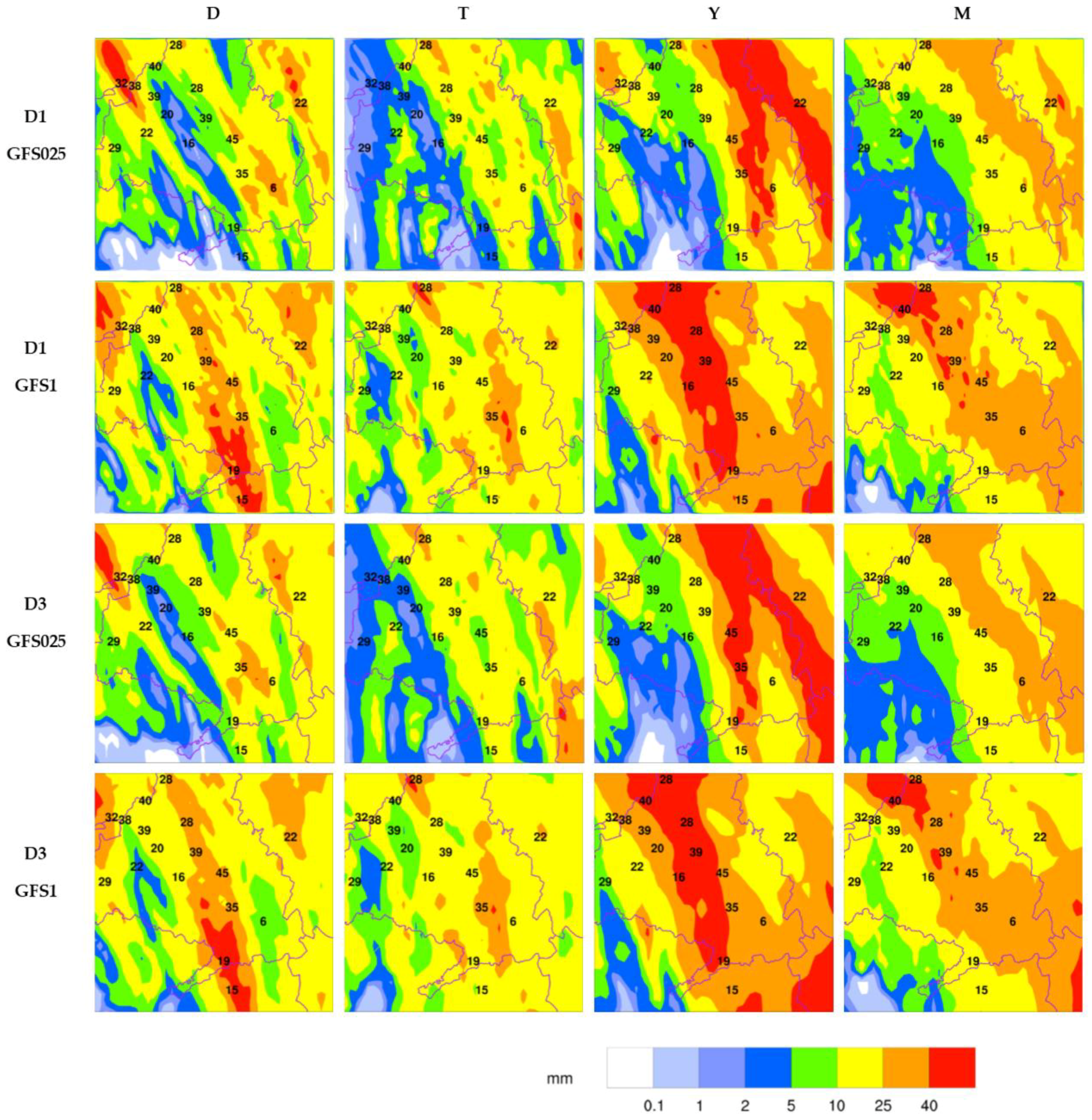
Regarding spatial precipitation distributions, total accumulated precipitation maps for deterministic model configurations (Figure 2) confirmed some of the results already mentioned. Considering the domain resolution, almost no difference was seen between D1 and D3 for the same physics scheme and GFS resolution. D3 appeared to produce slightly less precipitation than D1 (some red spots in D1 are smaller than in D3) and generated coarser rain fields, as may be expected because of grid size, but both domains were virtually the same. However, notable differences were observed for GFS resolutions. For the same domain resolution, GFS1 produced heavier precipitation than GFS025 (clearly observable in the D and M schemes). There was also a notable location/timing difference, as GFS025 produced rain fields to the east of GFS1 (clearly observable in the Y and M schemes). This displacement appears to be the main reason for the poorer results of GFS025.

When the simulated rainfall was compared to the observed accumulated precipitation values at each station (Figure 2), the results were somewhat coincidental with RBias values (Table 4). T underestimated the precipitation. T and M are the schemes that yielded fewer differences in rainfall between resolutions, and many simulations formed a bow-shaped heavy precipitation field (Figure 2). This was aligned in a north–south direction across the centre of the domain, with values dependent on the performance of the physics scheme; this is very evident from the Y scheme (red band). These figures also allow us to put in perspective the validation indices already assessed. The Y scheme always overestimated precipitation. Nevertheless, RBias for Y at the GFS025 resolution was negative (Table 4). Because of the validation indices calculated at the selected stations, the aforementioned displacement of the simulated rain fields radically altered RBias values depending on GFS resolution, with even RMAE and RRMSE very similar for all model configurations in the Y scheme.

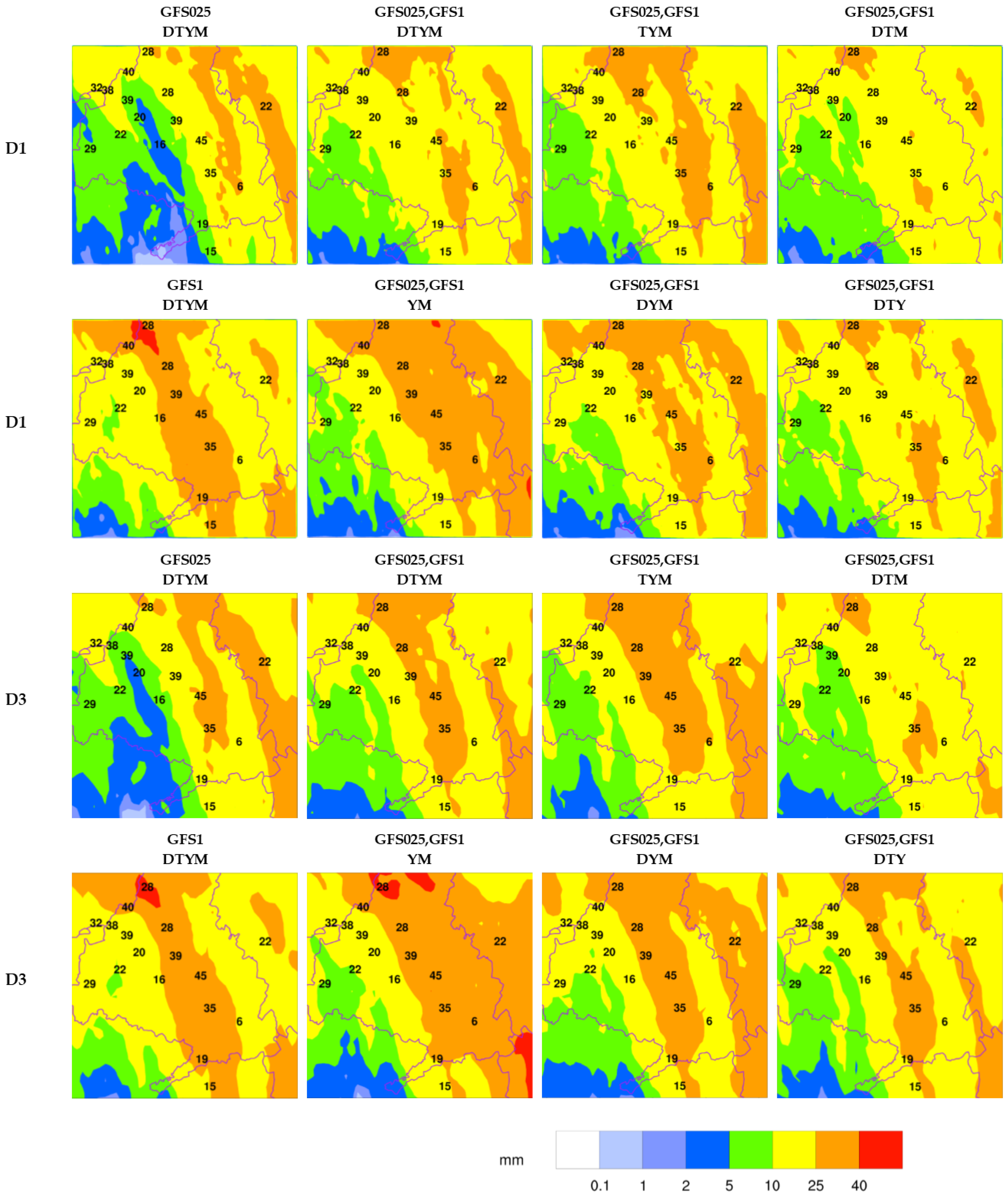
Total accumulated precipitation for ensemble model configurations (Figure 3) show similar results for the physics ensembles. For both D1 and D3, precipitation was simulated to the east and in lesser quantities for GFS025-DTYM than for GFS1-DTYM, producing a poorer validation of GFS025 configurations. No large differences were seen between domains for the same GFS resolution, but a coarser structure. When the initial conditions ensemble and additional ensembles merge the two GFS resolutions, the rain field location difference disappears, but the error in precipitation accumulation is reflected in the domains. D3 showed heavier precipitation than D1 for the same model configuration. This proves that, although negligible, there were small differences between domains, which can also be observed in the validation indices (Table 4). Because of the heavy precipitation simulated by the Y physics scheme (Figure 2), the model ensembles using it tended to reproduce a sharper bow pattern across the study area. A heavy precipitation core was consistently over the northern and central study area, whereas the southwestern corner showed little to no precipitation. The rest of the domain shows variable precipitation amounts but similar patterns, almost always displaying the bow shape seen in the deterministic configurations.

3.2. Validation of Temporal Evolution

The validation of r and number of statistically significant stations for the deterministic model configurations provided conclusive results (

Table 5. Temporal validation: r and number of statistically significant stations. All 32 model configurations are shown for domain resolution, GFS resolution, microphysics parameterizations, and various ensembles chosen. All r values are statistically significant. Best three performers for each index are shaded.

		Deterministic				Physics Ensemble	Initial Conditions Ensemble	Additional Ensembles
		D	T	Y	M	DTYM	DTYM	TYM	DYM	DTM	DTY	YM
r
D1	GFS025	0.465	0.340	0.430	0.533	0.541	0.592	0.598	0.616	0.565	0.544	0.632
	GFS1	0.269	0.386	0.501	0.645	0.554
D3	GFS025	0.444	0.328	0.299	0.498	0.462	0.554	0.541	0.581	0.552	0.500	0.570
	GFS1	0.265	0.400	0.513	0.652	0.562
Number of statistically significant stations
D1	GFS025	11	9	8	12	13	13	11	13	12	11	12
	GFS1	6	8	10	14	11
D3	GFS025	11	9	4	12	11	11	10	11	13	9	11
	GFS1	6	8	10	14	11

). The M scheme outperformed every other scheme. Even when compared with the ensemble configurations, the D3-GFS1-M and D1-GFS1-M achieved the best results for both r and number of statistically significant stations. Once again, GFS1 gave better results than GFS025 and there was little difference between D1 and D3. When initial conditions and additional ensembles were evaluated, the differences between domains were larger. Every r value was statistically significant and ensembles tended to perform better than deterministic configurations, clearly influenced by the M physics scheme. This was evident when the DTY ensemble results were compared to every other additional ensemble. Also, when the T scheme was removed (i.e., the DYM additional ensemble), results improved.

Considering the number of statistically significant stations (Table 5), similar results were obtained. Again, the M scheme produced the best results (up to 14 of the 17 stations with satisfactory results), and was not improved by any other deterministic configuration. Only some ensembles yielded better values than the GFS025-M configurations, but not better than GFS1-M configurations. The value of r index can be seen with the D1-GFS025-DTYM and D1-GFS1-DTYM physics ensembles. The produced r values were very similar, but GFS025 had 13 valid stations while GFS1 had only 11. Although the time correlation was slightly less, a model configuration with 13 valid stations was more robust and spatially consistent than one with 11 statistically significant stations out of 17. Similar results were obtained by ensembles D1-DTYM, D1-DYM, and D3-DTM, but never improving on the results of the deterministic D1-GFS1-M and D3-GFS1-M configurations.

3.3. Integrated Validation

Evaluating the integrated indices RAEC and RAAC (

Table 6. Integrated validation: RAEC and RAAC. All 32 model configurations are shown for domain resolution, GFS resolution, microphysics parameterizations, and various ensembles chosen. Best three performers for each index are shaded.

		Deterministic				Physics Ensemble	Initial Conditions Ensemble	Additional Ensembles
		D	T	Y	M	DTYM	DTYM	TYM	DYM	DTM	DTY	YM
RAEC
D1	GFS025	−0.220	−0.307	−0.140	−0.208	−0.219	−0.113	−0.121	−0.073	−0.150	−0.108	−0.065
	GFS1	0.053	−0.169	0.136	−0.042	−0.006
D3	GFS025	−0.229	−0.313	−0.154	−0.195	−0.233	−0.114	−0.122	−0.074	−0.150	−0.111	−0.065
	GFS1	0.050	−0.183	0.129	−0.050	−0.013
RAAC
D1	GFS025	0.279	0.354	0.345	0.325	0.298	0.254	0.259	0.242	0.260	0.261	0.243
	GFS1	0.310	0.299	0.319	0.208	0.252
D3	GFS025	0.287	0.355	0.293	0.337	0.302	0.260	0.263	0.250	0.270	0.264	0.247
	GFS1	0.310	0.305	0.317	0.210	0.249

), results were in accordance with the previous indices. The RAEC correlates well with RBias results (Table 4), and almost all RBias conclusions can be assumed. Best deterministic results were achieved by the D1-GFS1-M configuration, only outperformed by the physics ensemble initialized with GFS1. There was no significant difference between domain resolutions, but when initial conditions were evaluated, GFS1 performed better than GFS025. Nevertheless, some considerations must be made. It is remarkable that the D physics scheme overestimated precipitation when initialized with GFS1. This is contradictory to the RBias results for the same model configuration (Table 4), but it is the outcome of RAEC accounting for the entire validation period and not only for the results at its end. Also, when initial conditions and additional ensembles were considered, differences became smaller than those shown by RBias (Table 4).

The RAAC correlated well with RMAE results (Table 4), and once again almost all RMAE conclusions can be assumed as valid, with the M scheme initialized by GFS1 the best performer. The only remarkable difference with RMAE results was found for the D scheme. This physics scheme achieved better RMAE results with GFS1 initial conditions (Table 4), but RAAC gave a better outcome for GFS025. As was stated for RAEC, this was the product of evaluating the complete period of the simulation.

Overall, the best results were generated by the D1-GFS1-M deterministic configuration, which had the smallest error (RAAC) and was very well compensated (RAEC very close to 0). Although some ensemble configurations can improve RAEC, their RAACs were larger than the best deterministic configuration.

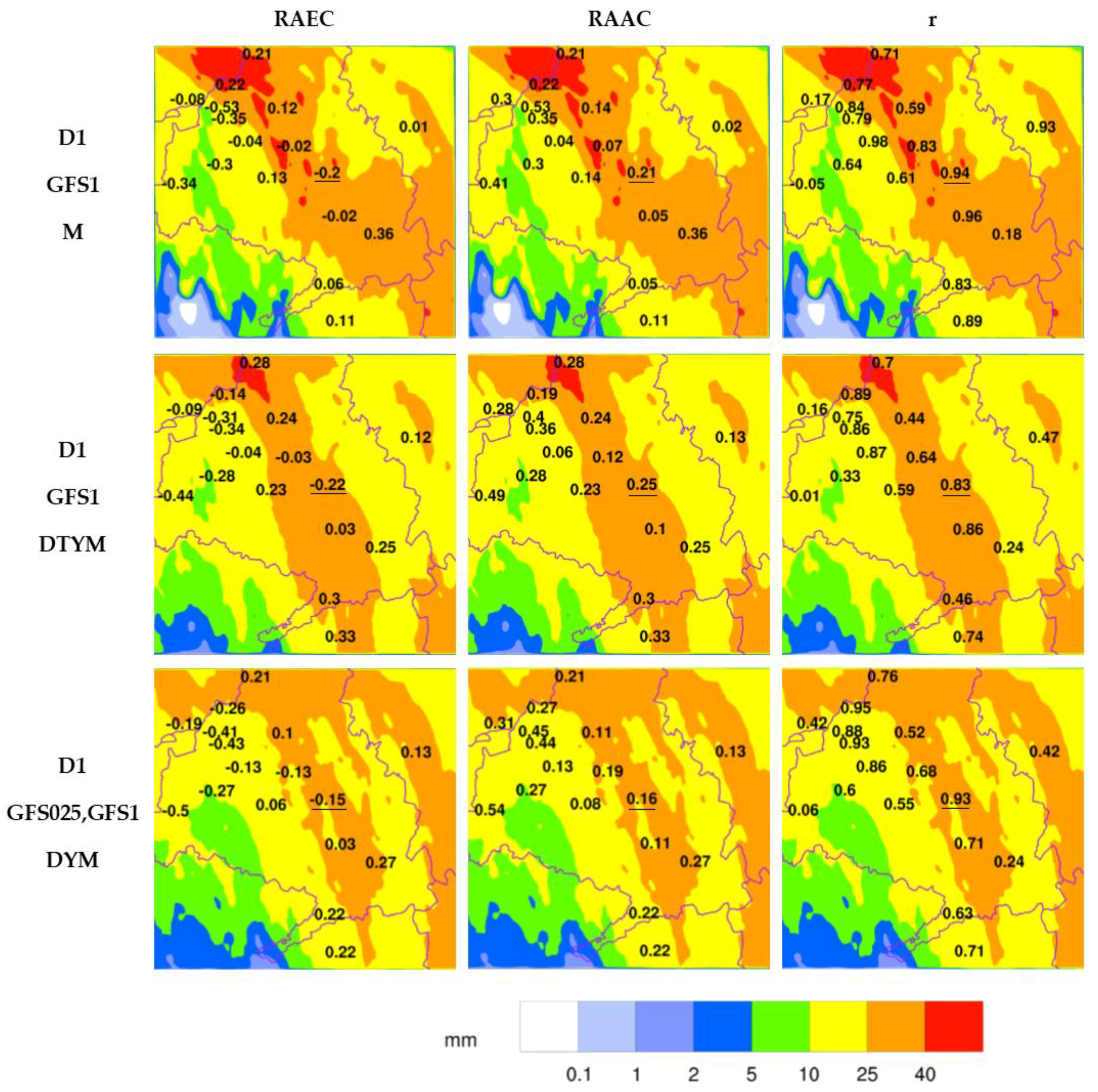
3.4. Spatial Assessment of Validation

For the spatial assessment of precipitation, three model configurations were selected, considering the overall best performers per the indices already presented. These are the deterministic D1-GFS1-M, physics ensemble D1-GFS1-DTYM, and additional ensemble D1-DYM. Upon initial analysis it was seen that the rainfall simulated by the selected configurations are similar (Figure 4), with three main features already mentioned. Those were a heavy precipitation bow-shaped band across the domain, a very heavy precipitation core to the north of the domain (not seen in the D1-DYM ensemble), and a light or zero precipitation area to the southwest. The largest differences between configurations were in the very heavy precipitation core and east of the domain, where the intensity of precipitation varied and even the bow-shaped band was duplicated by the D1-DYM ensemble.

Upon comparing the accumulated precipitation simulated values with observed values at the stations (Figure 4), it was evident that there were notable differences in RAEC and RAAC results for the same station, even when the station was within the same precipitation range (same colour in the rainfall image) for every selected configuration. This was a feature of the sensitivity of these indices. Evaluating RAEC results for a spatial assessment of precipitation, the most remarkable aspect was that every station near the mountains and west of the bow-shaped band (orange) tended to underestimate precipitation, whereas stations under or west of that band tended to overestimate (with two or three exceptions). Considering the RAAC results, it was seen that the area where stations tended to underestimate was also one with major error values. Also, the stations under the very heavy precipitation core have smaller RAAC values than those underestimated near the western part of the mountain range. This large underestimation error in the vicinity of the Guadarrama mountain range was possibly linked to an underestimation of the orographic enhancement of precipitation during this episode by the WRF model. The performance at station #11 was also remarkable, where the largest amount of precipitation of the event was observed. Here, the model underestimated with every selected configuration, even though we have seen that stations under the heavy precipitation bow-shaped band tended to overestimate. This location corresponds to LEMD and was analysed in the next section. Comparing RAEC and RAAC results, most of the stations did not compensate errors (the RAEC absolute value is similar to RAAC instead of near zero). This means that the errors at these stations were persistent over the period of validation, and the underestimation or overestimation of precipitation continued over time.

Concerning r values, there was good performance by the selected configurations. Most of the stations’ results were well above 0.5, with the deterministic D1-GFS1-M the best performer. Also, from r results, there was a consideration that can be extended to a complete spatial assessment. That is, owing to the nature of the event, a thorough interpretation of the data among the geographic domains must be performed, even on an individual station basis, for an integral validation of a model.

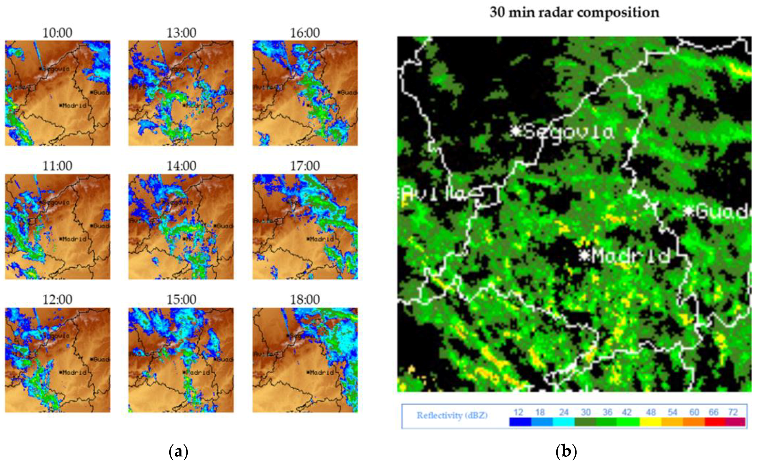
Not as an objective validation tool, but for comparison purposes, the radar reflectivity images were compared to the model simulations (Figure 5). The radar images show a convective system in a bow shape, entering the study area at ~10:00 UTC. It moved across the domain from southwest to northeast. At 14:00 UTC, the system reached the centre of the domain, over the city of Madrid, and remained there after 16:00 UTC. The persistence of rainfall in this area was estimated very accurately by most of the simulations, as shown by the bow shape of maximum accumulated precipitation (coloured in orange), which was repeatedly noted by Figure 2 and Figure 3. At 18:00 UTC, the system was well east of D1 and exiting the domain.

When the 30-min composite was analysed, three aspects were noted. There is an intense reflectivity core to the southwest of the domain, not captured by precipitation from any model configuration. There were no signs of high reflectivity to the north of the domain, where some model simulations tended to show a heavy precipitation core (although shadowing by terrain elevation should be considered in this case). There was a concentration of high reflectivity points in the centre of the domain, from the city of Madrid southward, which makes the bow shape in the model simulations consistent with reflectivity data. This proves that, as has already been stated, the simulations initialized by GFS025 displaces the bow-shaped maximum accumulated precipitation to the east, and that the model did not properly capture the precipitation near complex terrain and southwest of the domain. These may be the reasons why the validation of GFS025 model configurations gave poorer results and why the stations west of the domain had poor performance.

When 10-min images were analysed from 13:30 to 14:10 UTC (not shown), the development of an intense reflectivity cell (54 dBZ) that crossed LEMD was seen. In Figure 5, at 14:00 UTC this core had just passed over the airport. Later, two more cells traversed the area through 16:50 UTC, but with weaker reflectivity values. This is consistent with the observed precipitation at station #11 and was the cause for the disruption of airport operations during the day of the event.

3.5. LEMD Assessment

On the day studied, there were wind records suggestive of a wet microburst event over LEMD (not shown), which is a weather phenomenon very relevant to aircraft safety. Because this phenomenon depends largely on convective precipitation [31], there is a need to validate the precipitation simulation before attempting to simulate a microburst. Despite the marginal improvements and validation problems resulting from increasing model horizontal resolution, grid resolutions of 1 km and smaller may be required for the WRF to capture a microburst. Also, because the Thompson scheme is not the most suitable for convective precipitation, mid-altitude snow is an important factor for dry microbursts [32]. This is the reason for validating these model configurations over the area.

As presented in the previous section, although the general weather pattern or dynamics may be captured by a model, results cannot be generalised to every station. Because of scarce observed data, evaluation on individual basis should be performed for closer study, because this may be required for investigating a microburst. For this purpose, LEMD was chosen because it is the most important station for aviation safety in the study area (#11 in Figure 1b). In the evaluation of LEMD, additional ensembles were not considered.

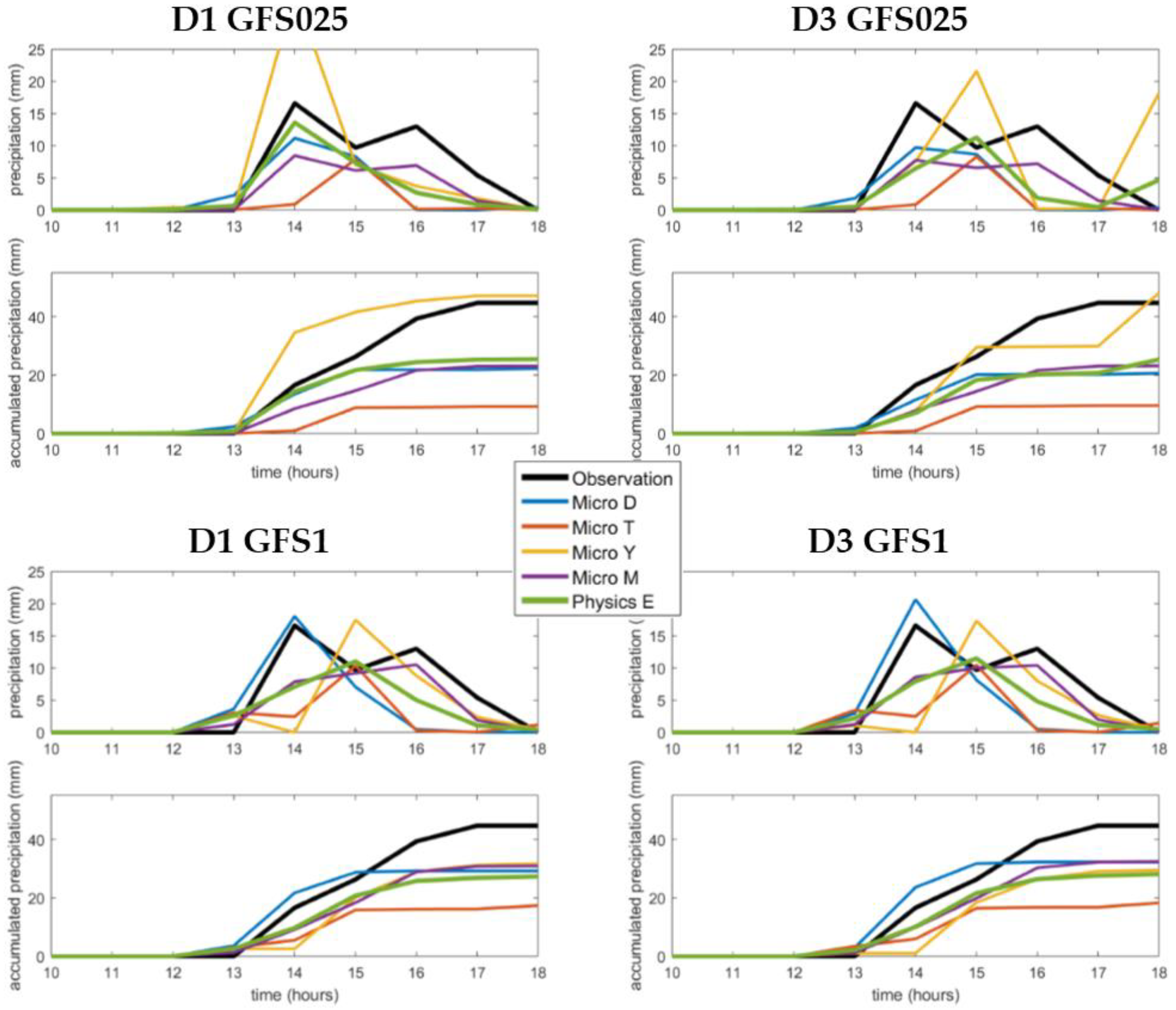
Studying every physics scheme performance for deterministic model configurations (Figure 6), several aspects were noted. Observations showed two precipitation maxima over the station, one at 14:00 and the second at 16:00 UTC, the first one with a slightly greater precipitation amount. GFS025 model configurations tended to simulate the precipitation onset at 13:00 UTC, whereas GFS1 configurations already simulated some rain at 12:00 UTC. The D, T, and M schemes generated more precipitation with the GFS1 configurations than with GFS025, with very little difference between domains. The Y scheme produced more precipitation with GFS025 than with the GFS1 configurations, and there were notable differences between domains when initialized by GFS025. The D physics scheme consistently produced a single maximum of hourly precipitation at 14:00 UTC. It captured very well the first maximum of observed precipitation, but did not reproduce the second, resulting in total accumulated precipitation underestimation. The T scheme showed a single maximum at 15:00 UTC, not coinciding with any of the maxima in observed values and with severe underestimation of total accumulated precipitation. The M scheme initialized by GFS025 was the only configuration that captured a two-maxima precipitation pattern, consistent with observations. GFS1 configurations showed a similar temporal evolution, with a heavy precipitation onset at 14:00 UTC but a single maximum at 16:00 UTC. This physics scheme underestimated precipitation with every model configuration, but appeared to be the best performer. The Y scheme was the most variable. It captured very well the total accumulated precipitation with GFS025, but underestimated with GFS1. Also, it produced a single maximum at 15:00 UTC with GFS1 for D1 and D3 (maxima at 13:00 UTC are negligible), a single maximum with D1-GFS025 at 14:00 UTC (showing severe overestimation), and a double maximum with D3-GFS025 at 15:00 and 18:00 UTC. All these LEMD results were consistent with the overall model results already presented.

It is remarkable that the observed data of accumulated precipitation (Figure 6) were sometimes outside the probability distribution function of the ensembles initialized by GFS1 (because observed accumulated precipitation was outside the range between the minimum and maximum simulated accumulated precipitation). This indicates that these ensembles are underdispersive. Although the validation results of simulations initialized by GFS025 were poorer than those of GFS1, by considering these simulations we may increase the ensemble spread, which can be interesting for detecting the risk of heavy precipitation at particular locations.

The temporal behaviour already detailed for each station is reflected in r values (

Table 7. LEMD station validation: RAAC, RAEC, and r values for a specific station. Only deterministic configurations, physics ensembles, and initial condition ensembles are shown. Values of r in parentheses denote a non-significant statistical result. Best three performers for each index are shaded.

		Deterministic				Physics Ensemble	Initial Conditions Ensemble
		D	T	Y	M	DTYM	DTYM
RAEC
D1	GFS025	−0.254	−0.521	0.197	−0.312	−0.222	−0.223
	GFS1	−0.098	−0.375	−0.215	−0.203	−0.223
D3	GFS025	−0.290	−0.516	−0.123	−0.315	−0.311	−0.261
	GFS1	−0.046	−0.361	−0.261	−0.177	−0.211
RAAC
D1	GFS025	0.274	0.522	0.197	0.313	0.230	0.238
	GFS1	0.198	0.402	0.238	0.214	0.246
D3	GFS025	0.306	0.517	0.172	0.316	0.317	0.274
	GFS1	0.183	0.392	0.271	0.188	0.231
r
D1	GFS025	0.754	(0.438)	0.809	0.987	0.880	0.896
	GFS1	0.764	(0.460)	0.553	0.938	0.833
D3	GFS025	0.745	(0.429)	(0.380)	0.979	0.670	0.777
	GFS1	0.774	(0.453)	0.554	0.943	0.843

). The T scheme results are statistically non-significant for every model configuration and the Y scheme values are small. Results for the M scheme were outstanding, with D1-GFS025-M the best performer. Ensemble configurations did not improve M results, but also produced very large values, especially for physics ensembles and D1 configurations. Considering RAEC and RAAC at LEMD (Table 7), it is evident that the D scheme performed very well with GFS1 and the Y scheme with GFS025. The M scheme results with D3-GFS1 were favourable, but overall results were mediocre.

We must note some factors regarding the favourable performance of the Y scheme with GFS025. It is important to recall that LEMD was the station with the largest observed precipitation values for the event, registering all its accumulated precipitation in just over three hours. This may be linked to a very heavy precipitation cell during that period. As has been mentioned, the Y scheme tended to overestimate overall precipitation and was not the best performer, but its overestimation improved the results of Y for this particular station and event.

The benefits of RAEC and RAAC can be seen by taking as examples the D and M schemes for the D1-GFS1 configuration. Total accumulated precipitation at the end of the validation period was essentially the same for both schemes, resulting in RBias values of −0.346 for D and −0.308 for M. It may seem that both schemes notably underestimated precipitation, but when time was considered, RAEC values showed that D (−0.098) underestimated considerably less than M (−0.203). This is confirmed by the accumulated precipitation behaviour (Figure 6), in which the D scheme overestimated precipitation from 13:00 to 15:00 UTC. The RMAE results were 0.553 for D and 0.493 for M. However, although at the end of the validation period these may be the errors, RAAC confirms that persistence of the error over the period was less for D (0.198) than for M (0.214). This means that the accumulated precipitation curve simulated by D remained closer to the observed curve vs. time, which is evident in the aforementioned figure.

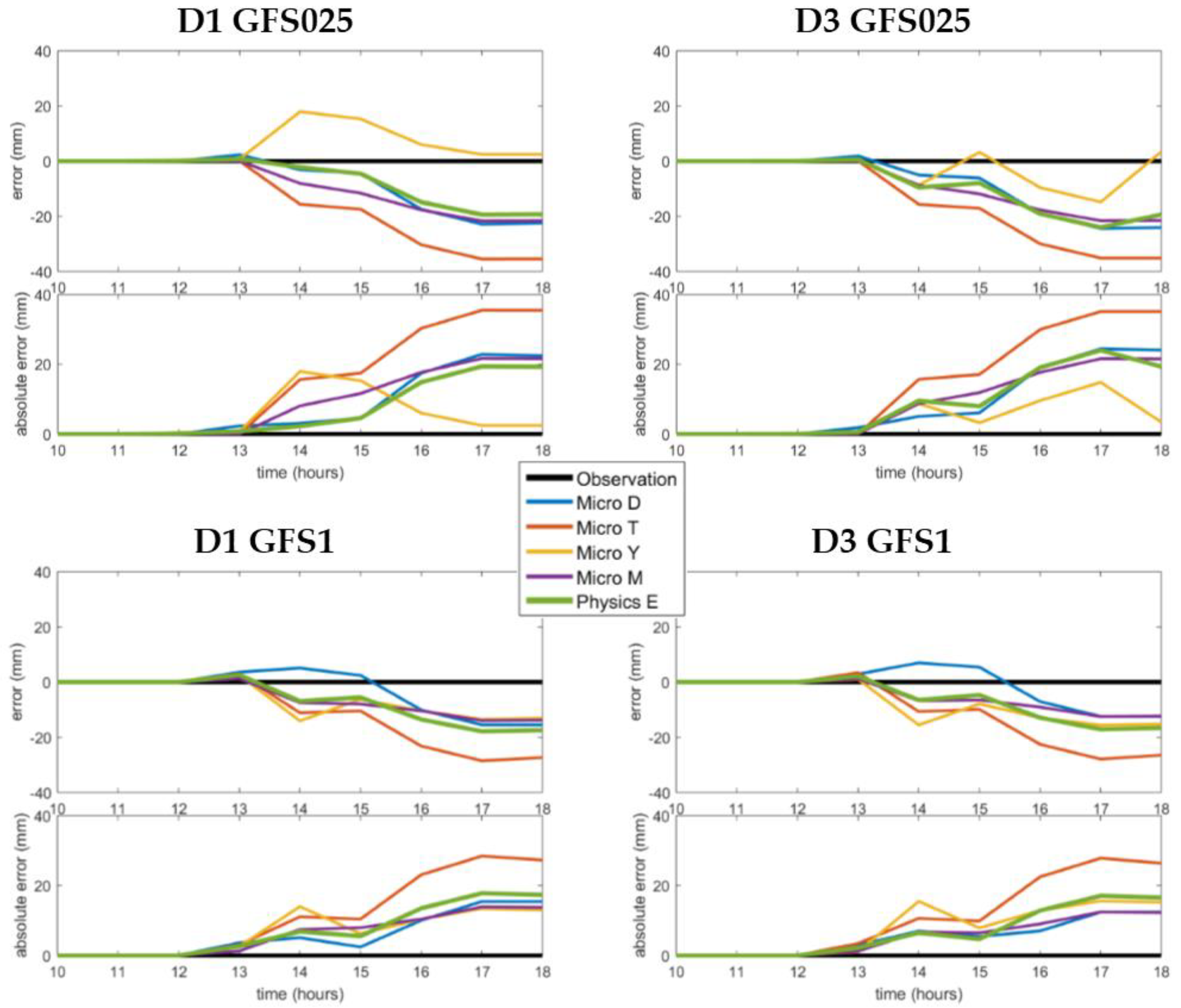
When the error curves were assessed (Figure 7), similar characteristics were found. These curves confirm that the best overall deterministic configurations for this station were D3-GFS1-D and D3-GFS1-M. GFS025 tended to create larger errors than GFS1 and there were almost no differences between domains. However, when the physics ensembles were evaluated it was discovered that the best performer was D1-GFS025, followed by D3-GFS1. This highlights that the improvements may be marginal and are strongly dependent on the exact model configuration.

4. Discussion and Conclusions

Considering the physics parameterizations, it is evident that the T scheme was not able to simulate this heavy precipitation event accurately. The results produced by this scheme were always outperformed by some other scheme using any index or configuration. Results of ensembles not considering the T scheme consistently improved the ensembles that did consider it. Thus, we concluded that the T scheme is not apt for simulating this episode. This is consistent with the fact that Thompson et al. [19] designed this parameterization mainly to simulate drizzle conditions. This microphysics scheme produces excessive numbers of small droplets, which are not appropriate for convective precipitation [33]. Nevertheless, the D configuration (which also uses the Thompson microphysics parameterizations) should be considered, although its performance may be the second poorest. This is a clear indication that precipitation simulations depend on several factors and model parameterizations, not only on microphysics. Nonetheless, evaluating only the microphysics, the results for the M physics scheme were clearly the best among the deterministic configurations, although as it consistently underestimated the precipitation. Especially when initialized with the GFS1 resolution, the M scheme produced some of the best results for every validation index. Morrison et al. [22] created a two-moment microphysics scheme specifically designed for storms, and the parameterizations were fine-tuned to simulate stratiform precipitation trailing a squall line. This particular feature explains very well the outstanding results of this scheme for temporal correlation (Table 5 and Table 7), and it was the only one that captured the two maxima of precipitation over LEMD (Figure 6). Also, this finding is consistent with the results obtained by García-Ortega et al. [8], who included the M scheme in the best-performing microphysics parameterizations in their analysis of convective precipitation over the Northeastern Iberian Peninsula. Validating the ensemble configurations, the best results are achieved by YM and DYM, with small differences between them. In case a configuration must be selected in future investigations, it should depend on the objective and needs of the study. A YM ensemble would be less computationally demanding, but a DYM ensemble would be more robust and consistent.

Evaluating domain resolution, D3 produced coarser rainfalls than D1, but only minor differences were found in the numerical results. The performance of domain resolution appears to depend on the exact model configuration. Nevertheless, D1 results were better for almost every index for the initial conditions and additional ensembles, but improvements were almost negligible. Schwartz et al. [34] reached this conclusion when they found no statistically significant differences between 4 km and 2 km grid resolutions for severe precipitation forecasting using WRF. Even before this, Kain et al. [35] had already questioned if downscaling from 4 km to 2 km would provide any added value to forecast skills. There are also other important considerations, because short-range simulations of convective weather validated against scarce and non-uniform data have serious challenges. The use of “traditional” validation scores for high-resolution simulations has been extensively questioned by Mass et al. [36] among others, mainly owing to the penalty that timing errors may generate. Pontoppidan et al. [37] concluded that complex terrain adds another source of error because of gravity wave representations, resulting in marginal improvement when downscaling resolution.

After assessing the GFS resolution, our results confirm that mesoscale models have a strong dependence and sensitivity to initial conditions [38]. Also, it is evident that the sensitivity of the model is greater for initial condition resolution than domain resolution. It is very interesting that GFS1 improved GFS025 results for almost every validation index, some being an order of magnitude better. In this case, the GFS1 initial conditions provided a more realistic representation of the rainfall field and precipitation amount than simulations initialized with GFS025. Also, the poor performance of GFS025 appeared to be largely affected by a timing/location error. Given that the majority of observing stations were west of the domain, the simulation of heavier precipitation displaced to the east had a great impact on scoring indices. Similar validation errors have been observed by Mass et al. [36], and timing differences for deep convection between domain resolutions have been described by Weisman et al. [39]. However, to our knowledge, timing errors for different resolutions of initial conditions produced by the same source have not been previously assessed. Nevertheless, such results are in agreement with those noted by Jee and Kim [17], who obtained better validation results initializing their model with initial conditions with horizontal resolution 1° × 1° than by initial conditions with much higher resolution. This suggests the need for improving data assimilation at the regional scale, especially by additional observational data sources.

As a general conclusion, physics parameterizations controlled the spatial distribution and quantity of precipitation simulated for the event, while initial conditions resolution affect the exact placement and timing of it. The domain resolution, being D1 and D3 having very high resolutions, had no significant effect. Other conclusions can be made. Bias, MAE, RMSE, and r values obtained are comparable to those of other works also simulating heavy precipitation events, e.g., Evans et al. [40] in Australia, García-Ortega et al. [8] in Spain, and Pontoppidan et al. [37] in Norway. Because of the poor validation scores of GFS025, the initial conditions and additional ensembles rarely outperformed the best physics ensemble or deterministic configuration. The only exception to this was the temporal correlation for D1, in which differences between GFS025 and GFS1 were smaller and the performance of the initial conditions and additional ensembles improved.

It is also important that although the GFS1 initial conditions and M physics scheme combination yielded outstanding results, the robustness and consistency produced by ensembles must be taken into account. An increase in ensemble spread may be attained by combining different physics parameterizations and initial conditions [41]. In this way, the underdispersive nature of the ensembles detected in the results can be partially corrected [42]. Therefore, although the best scores from the validation were obtained by the D1-GFS1-M configuration, the use of an ensemble provides additional information about the uncertainty associated with the spatiotemporal evolution of precipitation as well as the accumulated precipitation. Also, because underestimation of precipitation by numerical models is very common during convective episodes [43], a solution for the development of future early warning systems may be the use of ensemble maximum precipitation, in addition to the ensemble mean, with the aim of minimizing the underestimation.

The conclusions in this paper were reached by analysing a particular deep convection event in a specific region. They cannot be directly extrapolated to other regions or episodes. Therefore, we intend to evaluate similar episodes to obtain more robust conclusions about the optimal setup of the WRF model for forecasting this type of event. It was decided to examine this episode because of the serious disruptions it caused around the city of Madrid and especially at the LEMD airport.

We conclude with some other considerations about LEMD. The very heavy rain and gale-force wind gusts produced during the event forced the diversion and cancelation of several flights. As has been mentioned, these phenomena may be related to a microburst that the authors intend to analyse in detail in a later work. It is demonstrated by the present work that when a single location is evaluated, a unique assessment should be made, because model performance may vary greatly. Thus, the validation presented herein should be expanded and completed in future studies. Nevertheless, the results and methodology of the work can be very useful to develop early warning systems for minimizing the adverse effects of similar episodes in the study area.