Improving Quantitative Rainfall Prediction Using Ensemble Analogues in the Tropics: Case Study of Uganda

 , ,
, ,  ,
,  ,
,
Abstract
:1. Introduction
2. Data and Methods
2.1. Data Sources
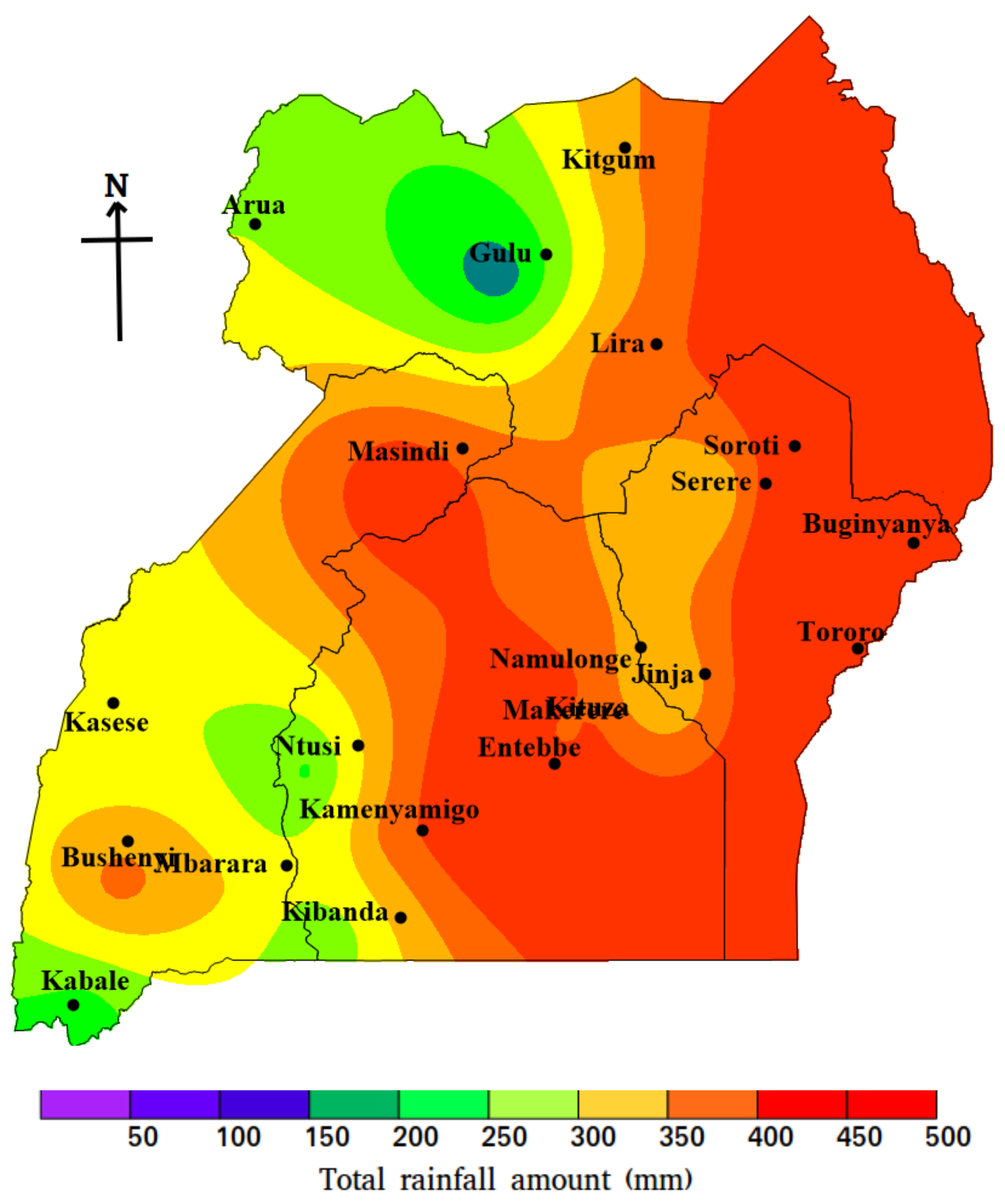
2.2. The Study Area
2.3. Experimental Design
- the first domain at a horizontal resolution of 90 km. This domain covered Africa and was deemed sufficiently enough to cover the large scale synoptic systems such as the sub–tropical high pressure systems which are important for rainfall over equatorial region;
- the second domain at a horizontal resolution of 30 km covering most parts of equatorial region to cater for the influx of moisture over Uganda especially the Congo air mass and the moist currents from Mozambique channel;
- the third domain at a horizontal resolution of 10 km covering Uganda, the study region. This domain was considered appropriate to resolve the local physical features like orography and the in–land water bodies.
2.4. Methods
2.4.1. Performance Analysis Methods
2.4.2. The Ensemble Mean
2.4.3. The Ensemble Mean Analogue
2.4.4. The Multi–Member Analogue Ensemble
2.4.5. Interpolation Method
3. Results and Discussion
3.1. Overview of the MAM Seasonal Rainfall Totals over Uganda
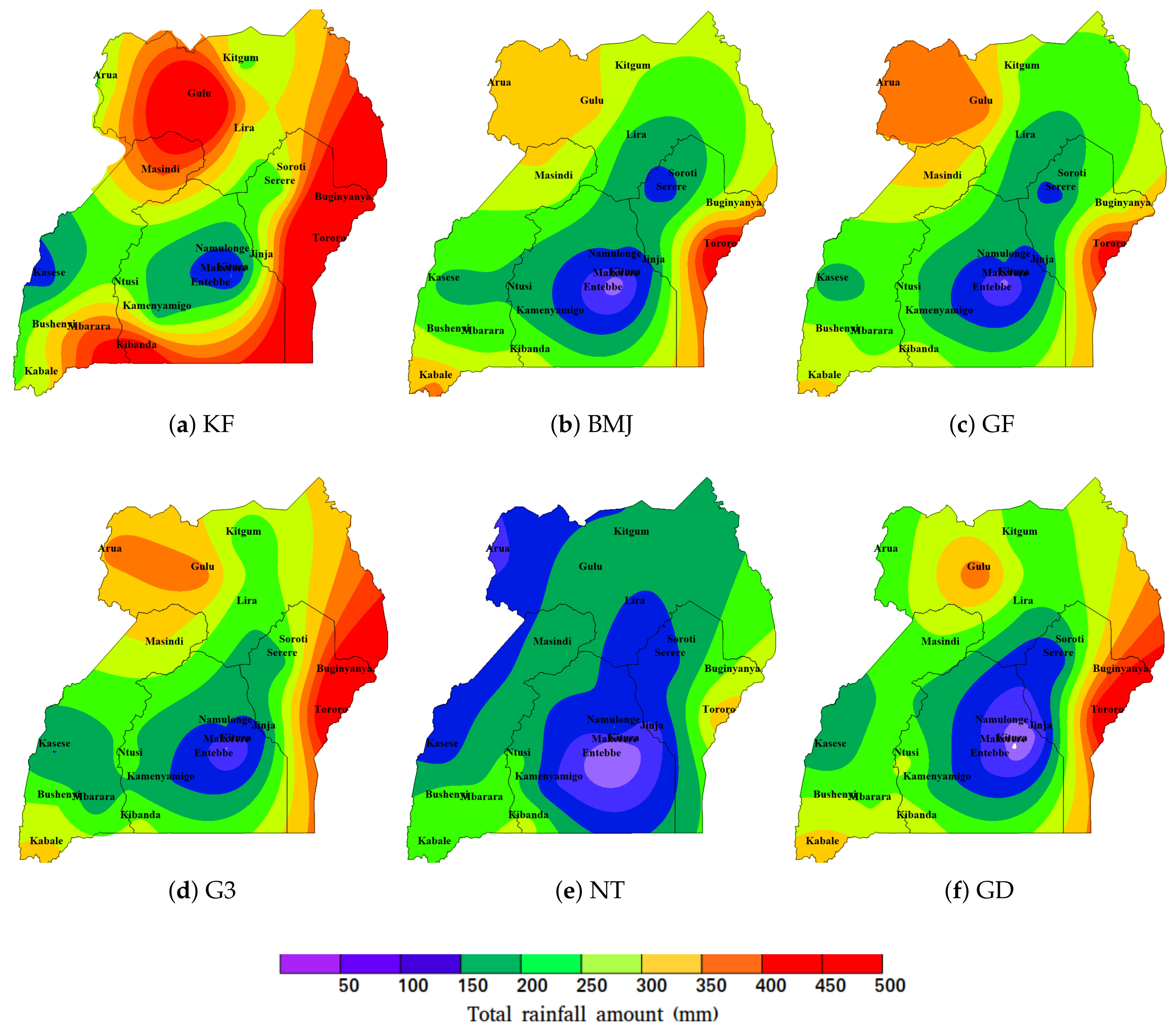
3.2. Performance of the Cumulus Schemes
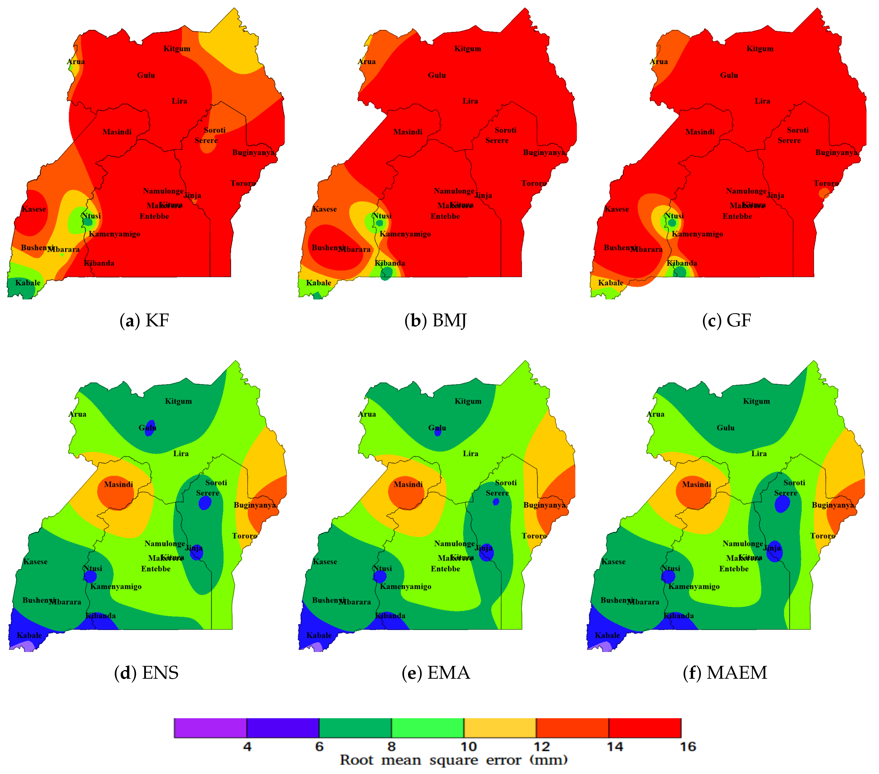
3.3. The Performance of Ensemble Mean
3.4. The Performance of Ensemble Mean Analogue
3.5. The Performance of Multi–Member Analogue Ensemble Method
4. Summary and Conclusions
Author Contributions
Acknowledgments
Conflicts of Interest
References
- Tao, S.; Shen, S.; Li, Y.; Wang, Q.; Gao, P.; Mugume, I. Projected crop production under regional climate change using scenario data and modeling: Sensitivity to chosen sowing date and cultivar. Sustainability 2016, 8, 214. [Google Scholar] [CrossRef]
- Ogwang, B.; Chen, H.; Li, X.; Gao, C. The influence of topography on east African October to December climate: Sensitivity experiments with REGCM4. Adv. Meteorol. 2014, 2014, 143917. [Google Scholar] [CrossRef]
- Karuri, S.W.; Snow, R.W. Forecasting paediatric malaria admissions on the Kenya Coast using rainfall. Glob. Health Action 2016, 9, 29876. [Google Scholar] [CrossRef] [PubMed] [Green Version]
- Kabo-Bah, A.T.; Diji, C.J.; Nokoe, K.; Mulugetta, Y.; Obeng-Ofori, D.; Akpoti, K. Multiyear rainfall and temperature trends in the Volta river basin and their potential impact on hydropower generation in Ghana. Climate 2016, 4, 49. [Google Scholar] [CrossRef]
- He, S.; Raghavan, S.; Nguyen, N.; Liong, S.-Y. Ensemble rainfall forecasting with numerical weather prediction and radar-based nowcasting models. Hydrol. Process. 2013, 27, 1560–1571. [Google Scholar] [CrossRef]
- Ntwali, D.; Ogwang, B.; Ongoma, V. The impacts of topography on spatial and temporal rainfall distribution over Rwanda based on WRF model. Atmos. Clim. Sci. 2016, 6, 145–157. [Google Scholar] [CrossRef]
- Awange, J.; Anyah, R.; Agola, N.; Forootan, E.; Omondi, P. Potential impacts of climate and environmental change on the stored water of Lake Victoria Basin and economic implications. Water Resour. Res. 2013, 49, 8160–8173. [Google Scholar] [CrossRef] [Green Version]
- Mugume, I.; Mesquita, M.; Basalirwa, C.; Bamutaze, Y.; Reuder, J.; Nimusiima, A.; Waiswa, D.; Mujuni, G.; Tao, S.; Jacob Ngailo, T. Patterns of dekadal rainfall variation over a selected region in lake victoria basin, Uganda. Atmosphere 2016, 7, 150. [Google Scholar] [CrossRef]
- Ngailo, T.; Shaban, N.; Reuder, J.; Rutalebwa, E.; Mugume, I. Non homogeneous poisson process modelling of seasonal extreme rainfall events in Tanzania. Int. J. Sci. Res. 2016, 5, 1858–1868. [Google Scholar]
- Jie, W.; Wu, T.; Wang, J.; Li, W.; Polivka, T. Using a deterministic time-lagged ensemble forecast with a probabilistic threshold for improving 6–15 day summer precipitation prediction in China. Atmos. Res. 2015, 156, 142–159. [Google Scholar] [CrossRef]
- Coiffier, J. Fundamentals of Numerical Weather Prediction; Cambridge University Press: Cambridge, UK, 2011. [Google Scholar]
- Mayor, Y.; Mesquita, M. Numerical simulations of the 1 May 2012 deep convection event over Cuba: Sensitivity to cumulus and microphysical schemes in a high-resolution model. Adv. Meteorol. 2015, 2015, 973151. [Google Scholar] [CrossRef]
- Maussion, F.; Scherer, D.; Finkelnburg, R.; Richters, J.; Yang, W.; Yao, T. WRF simulation of a precipitation event over the Tibetan Plateau, China—An assessment using remote sensing and ground observations. Hydrol. Earth Syst. Sci. 2011, 15, 1795–1817. [Google Scholar] [CrossRef]
- ECMWF. What Is Ensemble Weather Forecasting? 2017. Available online: https://www.ecmwf.int/en/about/media-centre/fact-sheet-ensemble-weather-forecasting (accessed on 24 October 2017).
- Glahn, H.R.; Lowry, D.A. The use of model output statistics (MOS) in objective weather forecasting. J. Appl. Meteorol. 1972, 11, 1203–1211. [Google Scholar] [CrossRef]
- Scheuerer, M. Probabilistic quantitative precipitation forecasting using ensemble model output statistics. Q. J. R. Meteorol. Soc. 2014, 140, 1086–1096. [Google Scholar] [CrossRef]
- Fraley, C.; Raftery, A.; Gneiting, T.; Sloughter, J.; Berrocal, V. Probabilistic weather forecasting in R. R. J. 2011, 3, 55–63. [Google Scholar]
- Mugume, I.; Basalirwa, C.; Waiswa, D.; Reuder, J.; Mesquita, M.D.S.; Tao, S.; Ngailo, T. Comparison of parametric and nonparametric methods for analyzing the bias of a numerical model. Model. Simul. Eng. 2016, 2016. [Google Scholar] [CrossRef]
- Gneiting, T.; Raftery, A. Weather forecasting with ensemble methods. Science 2005, 310, 248–249. [Google Scholar] [CrossRef] [PubMed]
- Hemri, S.; Scheuerer, M.; Pappenberger, F.; Bogner, K.; Haiden, T. Trends in the predictive performance of raw ensemble weather forecasts. Geophys. Res. Lett. 2014, 41, 9197–9205. [Google Scholar] [CrossRef] [Green Version]
- Whitaker, J.; Loughe, A. The relationship between ensemble spread and ensemble mean skill. Mon. Weather Rev. 1998, 126, 3292–3302. [Google Scholar] [CrossRef]
- Raftery, A.; Gneiting, T.; Balabdaoui, F.; Polakowski, M. Using Bayesian model averaging to calibrate forecast ensembles. Mon. Weather Rev. 2005, 133, 1155–1174. [Google Scholar] [CrossRef]
- Segele, Z.; Richman, M.; Leslie, L.; Lamb, P. Seasonal-to-interannual variability of Ethiopia/horn of Africa monsoon. Part II: Statistical multimodel ensemble rainfall predictions. J. Clim. 2015, 28, 3511–3536. [Google Scholar] [CrossRef]
- Evans, J.; Ji, F.; Abramowitz, G.; Ekström, M. Optimally choosing small ensemble members to produce robust climate simulations. Environ. Res. Lett. 2013, 8, 044050. [Google Scholar] [CrossRef] [Green Version]
- Zhu, J.; Kong, F.; Ran, L.; Lei, H. Bayesian model averaging with stratified sampling for probabilistic quantitative precipitation forecasting in northern China during summer 2010. Mon. Weather Rev. 2015, 143, 3628–3641. [Google Scholar] [CrossRef]
- Redmond, G.; Hodges, K.; Mcsweeney, C.; Jones, R.; Hein, D. Projected changes in tropical cyclones over Vietnam and the south China sea using a 25 km regional climate model perturbed physics ensemble. Clim. Dyn. 2015, 45, 1983–2000. [Google Scholar] [CrossRef]
- Fritsch, J.; Carbone, R. Improving quantitative precipitation forecasts in the warm season: A USWRP research and development strategy. Bull. Am. Meteorol. Soc. 2004, 85, 955–965. [Google Scholar] [CrossRef]
- Hamill, T.; Whitaker, J. Probabilistic quantitative precipitation forecasts based on reforecast analogs: Theory and application. Mon. Weather Rev. 2006, 134, 3209–3229. [Google Scholar] [CrossRef]
- Vanvyve, E.; Delle Monache, L.; Monaghan, A.; Pinto, J. Wind resource estimates with an analog ensemble approach. Renew. Energy 2015, 74, 761–773. [Google Scholar] [CrossRef]
- Kalnay, E.; Kanamitsu, M.; Kistler, R.; Collins, W.; Deaven, D.; Gandin, L.; Iredell, M.; Saha, S.; White, G.; Woollen, J.; et al. The NCEP/NCAR 40-year reanalysis project. Bull. Am. Meteorol. Soc. 1996, 77, 437–471. [Google Scholar] [CrossRef]
- White, D.; Lubulwa, G.; Menz, K.; Zuo, H.; Wint, W.; Slingenbergh, J. Agro-climatic classification systems for estimating the global distribution of livestock numbers and commodities. Environ. Int. 2001, 27, 181–187. [Google Scholar] [CrossRef]
- Basalirwa, C. Delineation of uganda into climatological rainfall zones using the method of principal component analysis. Int. J. Climatol. 1995, 15, 1161–1177. [Google Scholar] [CrossRef]
- Funk, C.; Hoell, A.; Shukla, S.; Husak, G.; Michaelsen, J. The east African monsoon system: Seasonal climatologies and recent variations. In The Monsoons and Climate Change; Springer: Berlin, Germany, 2016; pp. 163–185. [Google Scholar]
- Yang, W.; Seager, R.; Cane, M.; Lyon, B. The annual cycle of East African precipitation. J. Clim. 2015, 28, 2385–2404. [Google Scholar] [CrossRef]
- Pizarro, R.; Garcia-Chevesich, P.; Valdes, R.; Dominguez, F.; Hossain, F.; Ffolliott, P.; Olivares, C.; Morales, C.; Balocchi, F.; Bro, P. Inland water bodies in Chile can locally increase rainfall intensity. J. Hydrol. 2013, 481, 56–63. [Google Scholar] [CrossRef]
- Von Storch, H.; Zwiers, F.W. Statistical Analysis in Climate Research; Cambridge University Press: Cambridge, UK, 2003. [Google Scholar]
- Delle Monache, L.; Eckel, F.; Rife, D.; Nagarajan, B.; Searight, K. Probabilistic weather prediction with an analog ensemble. Mon. Weather Rev. 2013, 141, 3498–3516. [Google Scholar] [CrossRef]
- Horvath, K.; Bajić, A.; Ivatek-Šahdan, S.; Hrastinski, M.; Odak Plenković, I.; Stanešić, A.; Tudor, M.; Kovačić, T. Overview of meteorological research on the project “weather intelligence for wind energy”-will4wind. Hrvat. Meteorol. Čas. 2016, 50, 91–104. [Google Scholar]
- CPC. Cold and Warm Episodes by Season 2017. Available online: http://www.cpc.noaa.gov/products/analysis_monitoring/ensostuff/ensoyears.shtml (accessed on 1 February 2017).
- Hafez, Y. Study on the relationship between the oceanic nino index and surface air temperature and precipitation rate over the Kingdom of Saudi Arabia. J. Geosci. Environ. Prot. 2016, 4, 146–162. [Google Scholar] [CrossRef]
- Amiri, M.; Mesgari, M. Modeling the Spatial and Temporal Variability of Precipitation in Northwest Iran. Atmosphere 2017, 8, 254. [Google Scholar] [CrossRef]
- Franke, R. Scattered data interpolation: Tests of some methods. Math. Comput. 1982, 38, 181–200. [Google Scholar]
- Ratna, S.; Ratnam, J.; Behera, S.; Ndarana, T.; Takahashi, K.; Yamagata, T. Performance assessment of three convective parameterization schemes in WRF for downscaling summer rainfall over South Africa. Clim. Dyn. 2014, 42, 2931–2953. [Google Scholar] [CrossRef]


| RMSE Scores (mm) | RMSE Rankings | |||||||||||
|---|---|---|---|---|---|---|---|---|---|---|---|---|
| KF | BMJ | GF | G3 | NT | GD | KF | BMJ | GF | G3 | NT | GD | |
| Arua | 12.19 | 12.57 | 14.31 | 14.13 | 24.18 | 14.51 | 1 | 2 | 4 | 3 | 6 | 5 |
| Buginyanya | 19.66 | 58.76 | 59.51 | 33.10 | 62.66 | 42.89 | 1 | 4 | 5 | 2 | 6 | 3 |
| Bushenyi | 14.70 | 21.84 | 19.25 | 20.51 | 21.70 | 19.03 | 1 | 6 | 3 | 4 | 5 | 2 |
| Entebbe | 45.35 | 55.99 | 53.03 | 51.93 | 61.20 | 53.22 | 1 | 5 | 4 | 2 | 6 | 3 |
| Gulu | 57.98 | 17.49 | 24.05 | 23.04 | 6.53 | 25.21 | 6 | 2 | 4 | 3 | 1 | 5 |
| Jinja | 14.35 | 21.62 | 23.33 | 22.13 | 29.31 | 29.62 | 1 | 2 | 4 | 3 | 5 | 6 |
| Kibanda | 31.40 | 8.21 | 8.35 | 7.62 | 7.86 | 7.77 | 6 | 4 | 5 | 1 | 3 | 2 |
| Kabale | 8.19 | 15.95 | 10.04 | 11.31 | 6.28 | 13.00 | 2 | 6 | 3 | 4 | 1 | 5 |
| Kamenyamigo | 27.94 | 29.32 | 28.67 | 29.81 | 34.57 | 28.28 | 1 | 4 | 3 | 5 | 6 | 2 |
| Kasese | 19.18 | 14.63 | 15.43 | 18.02 | 19.27 | 16.72 | 5 | 1 | 2 | 4 | 6 | 3 |
| Kitgum | 16.44 | 14.69 | 16.31 | 18.33 | 24.77 | 18.32 | 3 | 1 | 2 | 5 | 6 | 4 |
| Kituza | 40.00 | 43.14 | 40.80 | 42.91 | 46.13 | 50.84 | 1 | 4 | 2 | 3 | 5 | 6 |
| Lira | 20.42 | 30.50 | 31.22 | 26.30 | 33.28 | 26.95 | 1 | 4 | 5 | 2 | 6 | 3 |
| Makerere | 33.76 | 43.77 | 42.71 | 41.29 | 46.78 | 37.59 | 1 | 5 | 4 | 3 | 6 | 2 |
| Mbarara | 11.73 | 18.17 | 18.80 | 22.16 | 18.68 | 15.68 | 1 | 3 | 5 | 6 | 4 | 2 |
| Masindi | 19.59 | 27.75 | 26.33 | 26.83 | 38.51 | 32.24 | 1 | 4 | 2 | 3 | 6 | 5 |
| Namulonge | 36.39 | 35.90 | 34.72 | 35.17 | 34.87 | 44.21 | 5 | 3 | 1 | 4 | 2 | 6 |
| Ntusi | 8.85 | 9.33 | 8.81 | 8.20 | 8.53 | 8.70 | 5 | 6 | 4 | 1 | 2 | 3 |
| Serere | 14.94 | 23.23 | 23.12 | 19.17 | 24.27 | 25.51 | 1 | 4 | 3 | 2 | 5 | 6 |
| Soroti | 16.08 | 27.62 | 25.25 | 18.84 | 28.24 | 25.93 | 1 | 5 | 3 | 2 | 6 | 4 |
| Tororo | 34.11 | 16.34 | 18.72 | 14.72 | 34.17 | 15.37 | 5 | 3 | 4 | 1 | 6 | 2 |
| Average | 23.96 | 26.04 | 25.85 | 24.07 | 29.13 | 26.27 | 2.38 | 3.71 | 3.43 | 3.00 | 4.71 | 3.76 |
| ME Scores (mm) | ME Rankings | |||||||||||
|---|---|---|---|---|---|---|---|---|---|---|---|---|
| KF | BMJ | GF | G3 | NT | GD | KF | BMJ | GF | G3 | NT | GD | |
| Arua | −0.89 | 0.91 | 1.83 | 1.20 | −4.49 | −1.97 | 1 | 2 | 4 | 3 | 6 | 5 |
| Buginyanya | −2.08 | −11.77 | −11.93 | −6.00 | −12.54 | −8.31 | 1 | 4 | 5 | 2 | 6 | 3 |
| Bushenyi | −2.19 | −4.03 | −3.22 | −3.78 | −3.99 | −3.34 | 1 | 6 | 2 | 4 | 5 | 3 |
| Entebbe | −9.06 | −11.36 | −10.73 | −10.50 | −12.44 | −10.77 | 1 | 5 | 3 | 2 | 6 | 4 |
| Gulu | 11.76 | 3.39 | 4.76 | 4.50 | 0.64 | 4.93 | 6 | 2 | 4 | 3 | 1 | 5 |
| Jinja | −2.15 | −4.14 | −4.58 | −4.31 | −5.89 | −5.93 | 1 | 2 | 4 | 3 | 5 | 6 |
| Kibanda | 6.22 | −0.04 | 0.53 | −0.18 | −0.08 | 0.34 | 6 | 1 | 5 | 3 | 2 | 4 |
| Kabale | 0.83 | 2.75 | 1.65 | 1.90 | 0.31 | 2.16 | 2 | 6 | 3 | 4 | 1 | 5 |
| Kamenyamigo | −5.31 | −5.58 | −5.50 | −5.76 | −6.78 | −5.46 | 1 | 4 | 3 | 5 | 6 | 2 |
| Kasese | −3.55 | −2.39 | −2.68 | −3.31 | −3.76 | −2.98 | 5 | 1 | 2 | 4 | 6 | 3 |
| Kitgum | −2.90 | −2.54 | −2.93 | −3.38 | −4.80 | −3.36 | 2 | 1 | 3 | 5 | 6 | 4 |
| Kituza | −7.94 | −8.57 | −8.08 | −8.53 | −9.23 | −10.24 | 1 | 4 | 2 | 3 | 5 | 6 |
| Lira | −3.43 | −5.85 | −6.00 | −4.94 | −6.51 | −5.11 | 1 | 4 | 5 | 2 | 6 | 3 |
| Makerere | −6.74 | −8.75 | −8.51 | −8.22 | −9.39 | −7.39 | 1 | 5 | 4 | 3 | 6 | 2 |
| Mbarara | 1.30 | −2.96 | −3.17 | −4.02 | −3.29 | −2.51 | 1 | 3 | 4 | 6 | 5 | 2 |
| Masindi | −2.34 | −4.63 | −4.29 | −4.50 | −7.26 | −5.78 | 1 | 4 | 2 | 3 | 6 | 5 |
| Namulonge | −7.22 | −7.06 | −6.82 | −6.89 | −6.83 | −8.81 | 5 | 4 | 1 | 3 | 2 | 6 |
| Ntusi | 0.32 | −0.98 | −0.54 | −0.55 | −0.48 | 0.47 | 1 | 6 | 4 | 5 | 3 | 2 |
| Serere | −2.61 | −4.53 | −4.51 | −3.66 | −4.78 | −5.04 | 1 | 4 | 3 | 2 | 5 | 6 |
| Soroti | −2.34 | −5.30 | −4.63 | −3.35 | −5.41 | −4.98 | 1 | 5 | 3 | 2 | 6 | 4 |
| Tororo | 6.30 | −1.40 | −2.51 | −1.80 | −6.58 | −1.49 | 5 | 1 | 4 | 3 | 6 | 2 |
| Average | −1.62 | −4.04 | −3.90 | −3.62 | −5.41 | −4.07 | 2.14 | 3.52 | 3.33 | 3.33 | 4.76 | 3.90 |
| Station | RMSE (mm) | ||
|---|---|---|---|
| ENS | EMA | MAEM | |
| Arua | 10.93 | 10.70 | 10.85 |
| Buginyanya | 15.23 | 15.36 | 15.02 |
| Bushenyi | 9.56 | 9.33 | 9.38 |
| Entebbe | 11.51 | 11.28 | 10.98 |
| Gulu | 7.78 | 7.76 | 8.04 |
| Jinja | 7.23 | 7.07 | 6.99 |
| Kabale | 5.81 | 5.92 | 5.87 |
| Kamenyamigo | 10.84 | 10.67 | 10.70 |
| Kasese | 8.37 | 8.21 | 8.28 |
| Kibanda | 6.91 | 6.89 | 6.90 |
| Kitgum | 8.34 | 8.96 | 8.32 |
| Kituza | 11.71 | 11.65 | 11.25 |
| Lira | 10.97 | 11.8 | 10.76 |
| Makerere | 11.02 | 10.83 | 10.63 |
| Masindi | 15.84 | 15.82 | 15.80 |
| Mbarara | 10.01 | 9.99 | 10.00 |
| Namulonge | 11.20 | 11.11 | 10.80 |
| Ntusi | 7.43 | 7.45 | 7.40 |
| Serere | 7.30 | 7.62 | 7.18 |
| Soroti | 9.83 | 10.16 | 9.84 |
| Tororo | 12.65 | 12.82 | 12.99 |
| Station | Mean Error (or Bias in mm) | ||
|---|---|---|---|
| ENS | EMA | MAEM | |
| Arua | 0.42 | 1.45 | 2.61 |
| Buginyanya | −2.92 | −2.02 | −0.54 |
| Bushenyi | −1.62 | −1.04 | −1.06 |
| Entebbe | −5.20 | −1.18 | −1.94 |
| Gulu | 4.08 | 4.26 | 5.13 |
| Jinja | −1.60 | −0.78 | 0.08 |
| Kabale | 0.57 | 1.00 | 1.25 |
| Kamenyamigo | −2.59 | −2.35 | −2.19 |
| Kasese | −1.49 | −1.04 | −0.76 |
| Kibanda | 0.89 | 0.56 | 1.15 |
| Kitgum | −1.02 | 0.15 | 0.94 |
| Kituza | −4.01 | −1.52 | −0.43 |
| Lira | −1.96 | 0.61 | 0.63 |
| Makerere | −3.92 | −2.50 | −1.39 |
| Masindi | −1.49 | −1.03 | −0.54 |
| Mbarara | −0.69 | −0.71 | −0.63 |
| Namulonge | −3.27 | −2.13 | −1.63 |
| Ntusi | 0.03 | −0.03 | 0.05 |
| Serere | −1.15 | 0.17 | 0.34 |
| Soroti | −0.94 | 0.52 | 1.39 |
| Tororo | 1.08 | 1.32 | 1.89 |
© 2018 by the authors. Licensee MDPI, Basel, Switzerland. This article is an open access article distributed under the terms and conditions of the Creative Commons Attribution (CC BY) license (http://creativecommons.org/licenses/by/4.0/).
Share and Cite
Mugume, I.; Mesquita, M.D.S.; Bamutaze, Y.; Ntwali, D.; Basalirwa, C.; Waiswa, D.; Reuder, J.; Twinomuhangi, R.; Tumwine, F.; Jakob Ngailo, T.; et al. Improving Quantitative Rainfall Prediction Using Ensemble Analogues in the Tropics: Case Study of Uganda. Atmosphere 2018, 9, 328. https://doi.org/10.3390/atmos9090328
Mugume I, Mesquita MDS, Bamutaze Y, Ntwali D, Basalirwa C, Waiswa D, Reuder J, Twinomuhangi R, Tumwine F, Jakob Ngailo T, et al. Improving Quantitative Rainfall Prediction Using Ensemble Analogues in the Tropics: Case Study of Uganda. Atmosphere. 2018; 9(9):328. https://doi.org/10.3390/atmos9090328
Chicago/Turabian StyleMugume, Isaac, Michel D. S. Mesquita, Yazidhi Bamutaze, Didier Ntwali, Charles Basalirwa, Daniel Waiswa, Joachim Reuder, Revocatus Twinomuhangi, Fredrick Tumwine, Triphonia Jakob Ngailo, and et al. 2018. "Improving Quantitative Rainfall Prediction Using Ensemble Analogues in the Tropics: Case Study of Uganda" Atmosphere 9, no. 9: 328. https://doi.org/10.3390/atmos9090328
APA StyleMugume, I., Mesquita, M. D. S., Bamutaze, Y., Ntwali, D., Basalirwa, C., Waiswa, D., Reuder, J., Twinomuhangi, R., Tumwine, F., Jakob Ngailo, T., & Ogwang, B. A. (2018). Improving Quantitative Rainfall Prediction Using Ensemble Analogues in the Tropics: Case Study of Uganda. Atmosphere, 9(9), 328. https://doi.org/10.3390/atmos9090328