A Comparison between 3DVAR and EnKF for Data Assimilation Effects on the Yellow Sea Fog Forecast


Abstract
:1. Introduction
2. Data Assimilation Algorithms
2.1. 3DVAR
2.2. EnKF
3. Numerical Experiments
3.1. Data
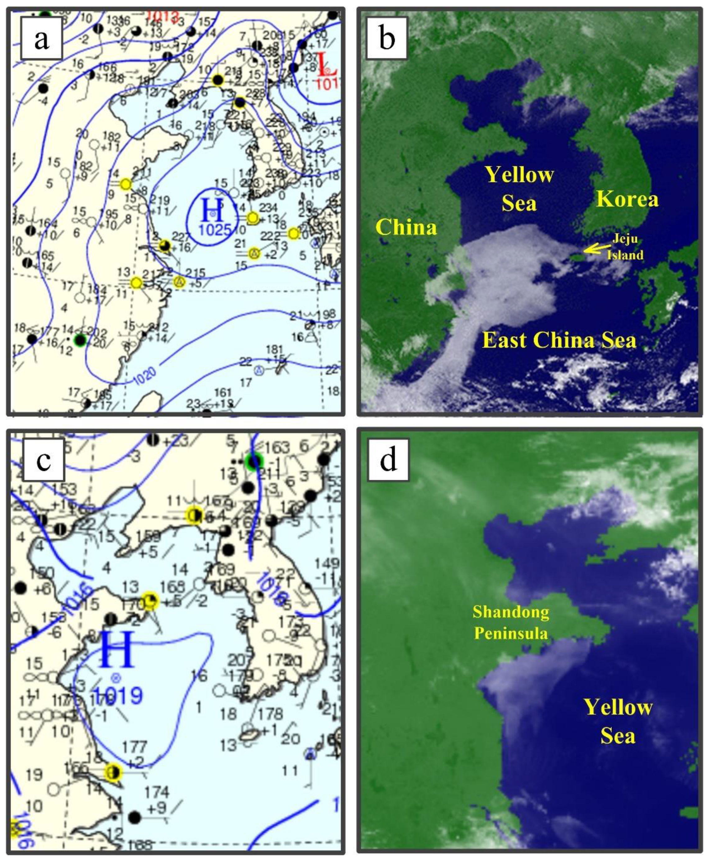
3.2. Sea Fog Cases
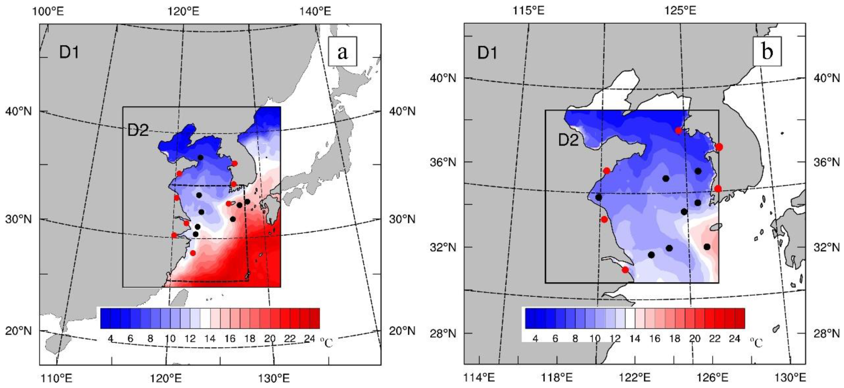
3.3. Model Configuration
3.4. Design of DA Schemes and Experiments
4. Results
4.1. Methods for Sea Fog Diagnostics and Evaluation
4.2. Evaluation of Assimilation Effect
4.2.1. Verification of Sea Fog Area
4.2.2. Verification by Measurements
4.3. Investigation of Assimilation Effects
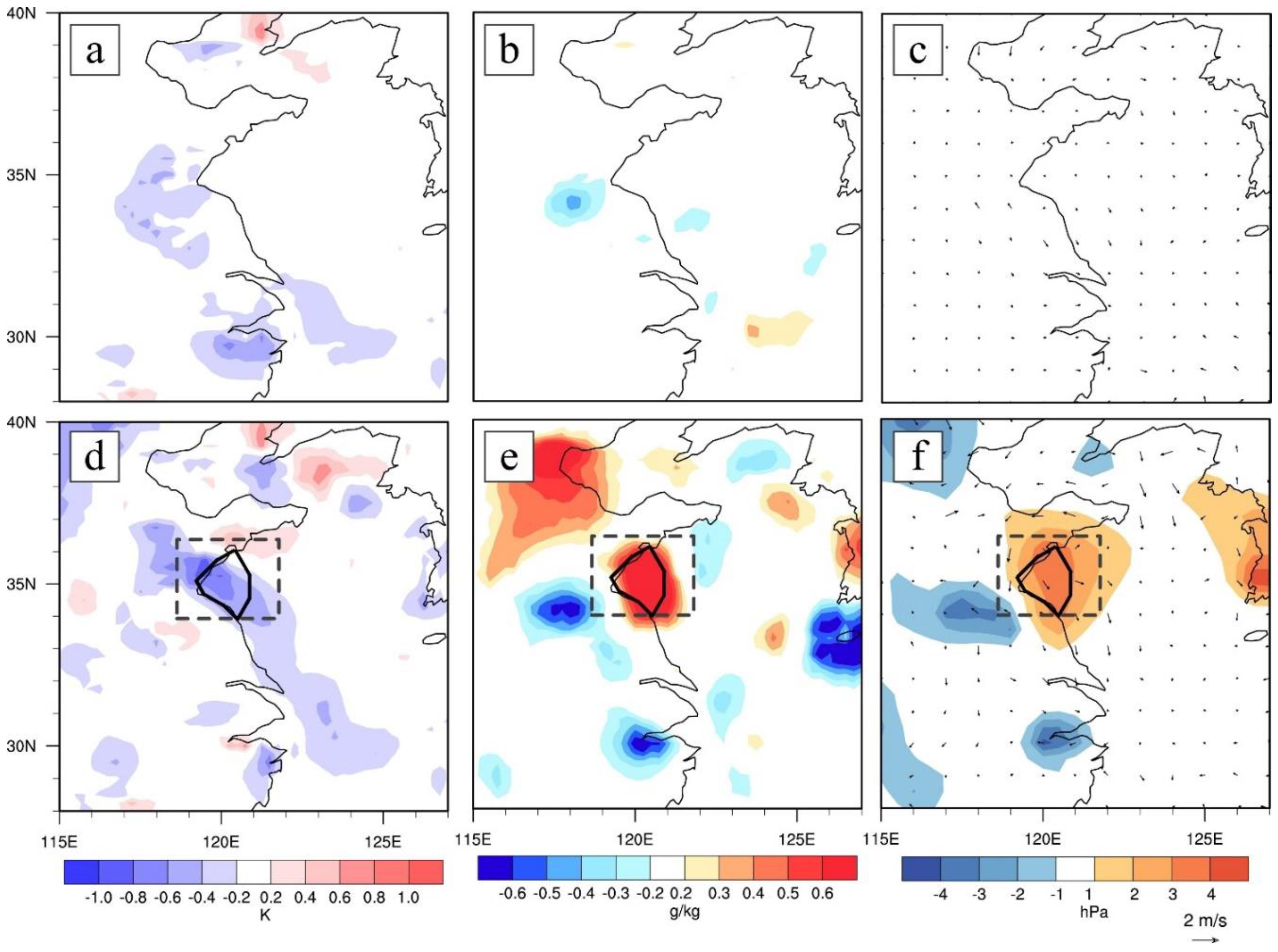
4.3.1. Feature of Initial Condition Differences
4.3.2. Reason for the Forecast Improvements
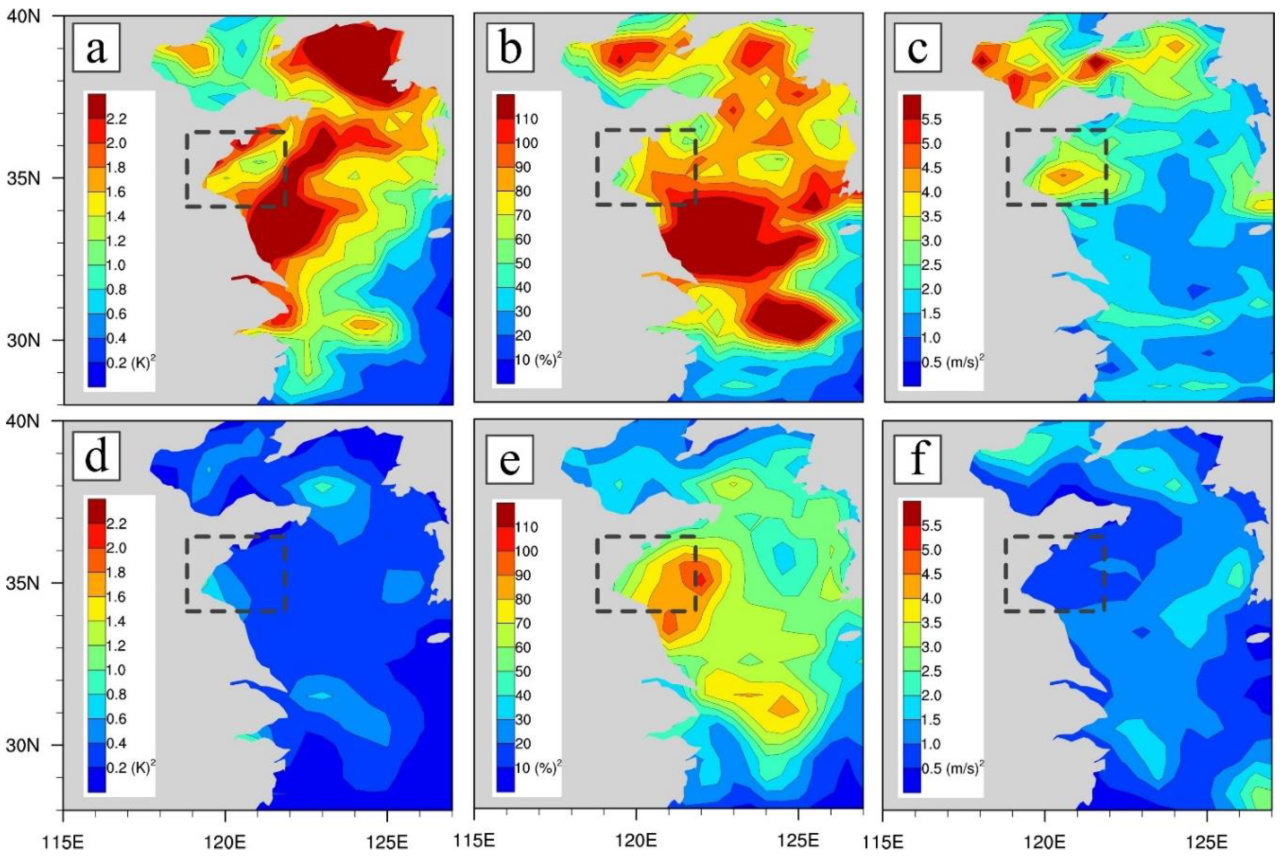
4.3.3. Impact of the Background Error Covariances
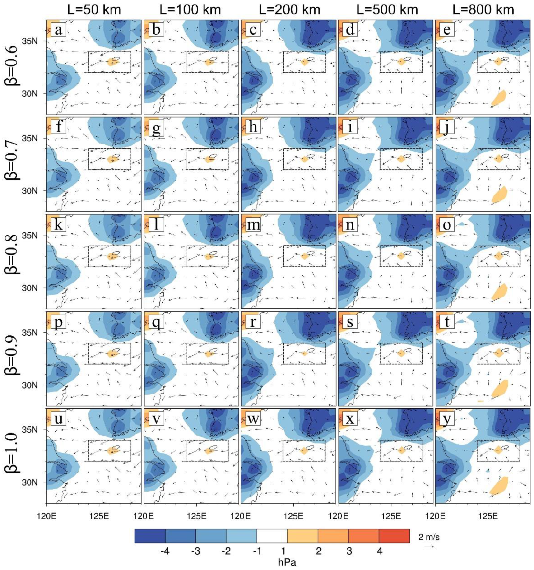
4.3.4. Sensitivity of Localization Scale and Inflation Factor
5. Conclusions
- (a)
- The assimilation effect of EnKF obviously excels that of 3DVAR, performing not only forecasted sea fog but also the distribution of temperature, moisture, and wind in the initial conditions. For the widespread-fog case, the assimilation by EnKF significantly improves the forecasted sea fog area, raising POD and ETS by up to about 57.9% and 55.5%, respectively. Especially for the case that spreads along the coast, the assimilation by EnKF successfully produces the sea fog formation which is completely mis-forecasted by 3DVAR.
- (b)
- The analysis increments strongly depend on the background error covariances. The flow-dependent background error covariances of EnKF out-compete that of 3DVAR, as evidenced by more realistic depiction of sea surface wind for the widespread-fog case and better existence of moisture for the other case in the initial conditions.
- (c)
- Compared with 3DVAR, the multivariate correlations (e.g., correlation between temperature and humidity) in the background error covariances of EnKF play a key role in adjusting/generating moisture through assimilation of temperature. This helps greatly to improve the moisture conditions for sea fog forecast.
- (d)
- A series of sensitivity experiments of EnKF shows that the forecast result is sensitive to ensemble inflation and localization factors, in particular, highly sensitive to the latter. These factors need to be tuned case by case or an adaptive localization method should be considered.
Author Contributions
Funding
Acknowledgments
Conflicts of Interest
References
- Wang, B.H. Sea Fog, 1st ed.; China Ocean Press: Beijing, China, 1985. [Google Scholar]
- Koračin, D.; Dorman, C.E. Marine Fog: Challenges and Advancements in Observations, Modeling, and Forecasting, 1st ed.; Springer International Publishing: New York, NY, USA, 2017; pp. 1–6. [Google Scholar]
- Gao, S.H.; Lin, H.; Shen, B.; Fu, G. A heavy sea fog event over the Yellow Sea in March 2005: Analysis and numerical modeling. Adv. Atmos. Sci. 2007, 24, 65–81. [Google Scholar] [CrossRef]
- Zhang, S.P.; Xie, S.P.; Liu, Q.Y.; Yang, Y.Q.; Wang, X.G.; Ren, Z.P. Seasonal variations of Yellow Sea fog: Observations and mechanisms. J. Clim. 2009, 22, 6758–6772. [Google Scholar] [CrossRef]
- Wang, Y.M.; Gao, S.H.; Fu, G.; Sun, J.L.; Zhang, S.P. Assimilating MTSAT-derived humidity in nowcasting sea fog over the Yellow Sea. Weather Forecast. 2014, 29, 205–225. [Google Scholar] [CrossRef]
- Fu, G.; Li, P.Y.; Zhang, S.P.; Gao, S.H. A Brief Overview of the Sea Fog Study in China. Adv. Meteorol. Sci. Tech. 2016, 6, 20–28. (In Chinese) [Google Scholar]
- Nicholls, S. The dynamics of stratocumulus: Aircraft observation and comparison with a mixed layer model. Q. J. Roy. Meteorol. Soc. 1984, 110, 783–820. [Google Scholar] [CrossRef]
- Findlater, J.; Roach, W.T.; McHugh, B.C. The haar of north-east Scotland. Q. J. Roy. Meteorol. Soc. 1989, 115, 581–608. [Google Scholar] [CrossRef]
- Ballard, S.P.; Golding, B.W.; Smith, R.N.B. Mesoscale model experimental forecasts of the haar of northeast Scotland. Mon. Weather Rev. 1991, 119, 2107–2123. [Google Scholar] [CrossRef]
- Lewis, J.M.; Koračin, D.; Rabin, R.; Businger, J. Sea fog off the California coast: Viewed in the context of transient weather systems. J. Geophys. Res. 2003, 108, 4457. [Google Scholar] [CrossRef]
- Koračin, D.; Lewis, J.; Thompson, W.T.; Dorman, C.E.; Businger, J.A. Transition of stratus into fog along the California coast: Observation and modeling. J. Atmos. Sci. 2001, 58, 1714–1731. [Google Scholar] [CrossRef]
- Koračin, D.; Businger, J.A.; Dorman, C.E.; Lewis, J.M. Formation, evolution, and dissipation of coastal sea fog. Bound. Layer Meteorol. 2005, 117, 447–478. [Google Scholar] [CrossRef]
- Koračin, D.; Leipper, D.F.; Lewis, J.M. Modeling sea fog on the U.S. California coast during a hot spell event. Geofizika 2005, 22, 59–82. [Google Scholar]
- Fu, G.; Guo, J.T.; Xie, S.P.; Duan, Y.H.; Zhang, M.G. Analysis and high-resolution modeling of a dense sea fog event over the Yellow Sea. Atmos. Res. 2006, 81, 292–303. [Google Scholar] [CrossRef]
- Gao, S.H.; Qi, Y.L.; Zhang, S.B.; Fu, G. Initial conditions improvement of sea fog numerical modeling over the Yellow Sea by using cycling 3DVAR. Part I: WRF numerical experiments. J. Ocean Univ. China 2010, 40, 1–9. (In Chinese) [Google Scholar]
- Liu, Y.D.; Ren, J.P.; Zhou, X. The impact of assimilating sea surface wind aboard QuikSCAT on sea fog simulation. J. Appl. Meteorol. Sci. 2011, 22, 472–481. (In Chinese) [Google Scholar]
- Li, R.; Gao, S.H.; Wang, Y.M. Numerical study on direct assimilation of satellite radiances for sea fog over the Yellow Sea. J. Ocean Univ. China 2012, 42, 10–20. (In Chinese) [Google Scholar]
- Wang, Y.M.; Gao, S.H. Assimilation of Doppler Radar radial velocity in Yellow Sea fog numerical modeling. J. Ocean Univ. China 2016, 46, 1–12. (In Chinese) [Google Scholar]
- Wang, J.J.; Gao, X.Y.; Gao, S.H. Data assimilation experiments and formation mechanism study of a Yellow Sea fog event. J. Marine Meteorol. 2017, 37, 42–53. (In Chinese) [Google Scholar]
- Parrish, D.F.; Derber, J.C. The National Meteorological Center’s spectral statistical-interpolation analysis system. Mon. Weather Rev. 1992, 120, 1747–1763. [Google Scholar] [CrossRef]
- Bouttier, F. A dynamical estimation of forecast error covariances in an assimilation system. Mon. Weather Rev. 1994, 122, 2376–2390. [Google Scholar] [CrossRef]
- Hamill, T.M.; Snyder, C. A hybrid ensemble Kalman filter-3D variational analysis scheme. Mon. Weather Rev. 2000, 128, 2905–2919. [Google Scholar] [CrossRef]
- Wang, X.G.; Barker, D.M.; Snyder, C.; Hamill, T.M. A hybrid ETKF-3DVAR data assimilation scheme for the WRF model. Part I: Observing system simulation experiment. Mon. Weather Rev. 2008, 136, 5116–5131. [Google Scholar] [CrossRef]
- Wang, X.G.; Barker, D.M.; Snyder, C.; Hamill, T.M. A hybrid ETKF-3DVAR data assimilation scheme for the WRF model. Part II: Real observation experiments. Mon. Weather Rev. 2008, 136, 5132–5147. [Google Scholar] [CrossRef]
- Talagrand, O.; Courtier, P. Variational assimilation of meteorological observations with the adjoint vorticity equation. I: Theory. Q. J. Roy. Meteorol. Soc. 1987, 113, 1311–1328. [Google Scholar] [CrossRef]
- Courtier, P.; Talagrand, O. Variational assimilation of meteorological observations with the adjoint vorticity equation. II: Numerical Results. Q. J. Roy. Meteorol. Soc. 1987, 113, 1329–1347. [Google Scholar] [CrossRef]
- Evensen, G. Sequential data assimilation with a nonlinear quasi-geostrophic model using Monte Carlo methods to forecast error statistics. J. Geophys. Res. Oceans 1994, 99, 10143–10162. [Google Scholar] [CrossRef]
- Yuan, B.; Fei, J.F.; Wang, Y.F.; Lu, Q. 4DVAR numerical simulation analysis using ATOVS data and asymmetrical bogus data on landing typhoon Weipha. Meteorol. Mon. 2010, 36, 13–20. (In Chinese) [Google Scholar]
- Wang, X.G. Application of the WRF hybrid ETKF-3DVAR data assimilation system for hurricane track forecasts. Weather Forecast. 2011, 26, 868–884. [Google Scholar] [CrossRef]
- Poterjoy, J.; Zhang, F. Intercomparison and coupling of ensemble and four-dimensional variational data assimilation methods for the analysis and forecasting of hurricane Karl (2010). Mon. Weather Rev. 2014, 142, 3347–3364. [Google Scholar] [CrossRef]
- Shen, F.F.; Min, J.Z.; Xu, D.M. Assimilation of radar radial velocity data with the WRF Hybrid ETKF–3DVAR system for the prediction of Hurricane Ike (2008). Atmos. Res. 2016, 169, 127–138. [Google Scholar] [CrossRef]
- Lu, X.; Wang, X.G.; Li, Y.Z.; Ma, X.L. GSI-based ensemble-variational hybrid data assimilation for HWRF for hurricane initialization and prediction: Impact of various error covariances for airborne radar observation assimilation. Q. J. Roy. Meteorol. Soc. 2017, 143, 223–239. [Google Scholar] [CrossRef]
- Yang, Y.; Gao, S.H. Analysis on the synoptic characteristics and inversion layer formation of the Yellow Sea fogs. J. Ocean Univ. China 2015, 45, 19–30. (In Chinese) [Google Scholar]
- Gultepe, I.; Tardif, R.; Michaelides, S.C.; Cermak, J.; Bott, A.; Bendix, J.; Müller, M.D.; Pagowski, M.; Hansen, B.; Ellrod, G.; et al. Fog research: A review of past achievements and future perspectives. Pure Appl. Geophys. 2007, 164, 1121–1159. [Google Scholar] [CrossRef]
- Shao, H.; Derber, J.; Huang, X.Y.; Hu, M.; Newman, K.; Stark, D.; Lueken, M.; Zhou, C.; Nance, L.; Kuo, Y.H.; et al. Bridging research to operations transitions: Status and plans of community GSI. Bull. Am. Meteorol. Soc. 2016, 97, 1427–1440. [Google Scholar] [CrossRef]
- Courtier, P.; Thépaut, J.N.; Hollingsworth, A. A strategy for operational implementation of 4D-Var, using an incremental approach. Q. J. Roy. Meteorol. Soc. 1994, 120, 1367–1387. [Google Scholar] [CrossRef]
- Waller, J.A.; Dance, S.L.; Lawless, A.S.; Nichols, N.K.; Eyre, J.R. Representativity error for temperature and humidity using the Met Office high-resolution model. Q. J. Roy. Meteorol. Soc. 2014, 140, 1189–1197. [Google Scholar] [CrossRef]
- Janjić, T.; Bormann, N.; Bocquet, M.; Carton, J.A.; Cohn, S.E.; Dance, S.L.; Losa, S.N.; Nichols, N.K.; Potthast, R.; Waller, J.A.; et al. On the representation error in data assimilation. Q. J. Roy. Meteorol. Soc. 2017. [Google Scholar] [CrossRef]
- Whitaker, J.S.; Hamill, T.M. Ensemble data assimilation without perturbed observations. Mon. Weather Rev. 2002, 130, 1913–1924. [Google Scholar] [CrossRef]
- Anderson, J.L.; Anderson, S.L. A Monte Carlo implementation of the nonlinear filtering problem to produce ensemble assimilations and forecasts. Mon. Weather Rev. 1999, 127, 2741–2758. [Google Scholar] [CrossRef]
- Houtekamer, P.L.; Zhang, F.Q. Review of ensemble Kalman filter for atmosphere data assimilation. Mon. Weather Rev. 2016, 144, 4489–4532. [Google Scholar] [CrossRef]
- Whitaker, J.S.; Hamill, T.M. Evaluating methods to account for system errors in ensemble data assimilation. Mon. Weather Rev. 2012, 140, 3078–3089. [Google Scholar] [CrossRef]
- Houtekamer, P.L.; Mitchell, H.L. A sequential ensemble Kalman filter for atmospheric data assimilation. Mon. Weather Rev. 2001, 129, 123–137. [Google Scholar] [CrossRef]
- Gaspari, G.; Cohn, S.E. Construction of correlation functions in two and three dimensions. Q. J. R. Meteorol. Soc. 1999, 125, 723–757. [Google Scholar] [CrossRef] [Green Version]
- MTSAT Data Archive. Available online: http://weather.is.kochi-u.ac.jp/sat/GAME (accessed on 15 November 2017).
- NCEP Final Analysis Data Archive. Available online: https://rda.ucar.edu/datasets/ds083.2 (accessed on 12 October 2017).
- NEAR-GOOS Dataset. Available online: http://ds.data.jma.go.jp/gmd/goos/data (accessed on 12 October 2017).
- NCEP GDAS Satellite Data. Available online: https://rda.ucar.edu/datasets/ds735.0 (accessed on 6 November 2017).
- CCMP Wind Vector Analysis Product. Available online: http://www.remss.com/measurements/ccmp (accessed on 25 February 2018).
- NCEP ADP Global Upper Air and Surface Weather Observations. Available online: https://rda.ucar.edu/datasets/ds337.0 (accessed on 25 February 2018).
- Skamarock, W.C.; Klemp, J.B.; Dudhia, J.; Gill, D.O.; Barker, D.M.; Duda, M.G.; Huang, X.Y.; Wang, W.; Powers, J.G. A Description of the Advanced Research WRF Version 3. Available online: http://www2.mmm.ucar.edu/wrf/users/docs/arw_v3.pdf (accessed on 10 January 2017).
- Lu, X.; Gao, S.H.; Rao, L.J.; Wang, Y.M. Sensitivity study of WRF parameterization schemes for the spring sea fog in the Yellow Sea. J. Appl. Meteorol. Sci. 2014, 25, 312–320. (In Chinese) [Google Scholar]
- Hong, S.Y.; Lim, K.S.; Kim, J.H.; Lim, J.O.J.; Dudhia, J. The WRF single-moment 6-class microphysics scheme (WSM6). J. Korean Meteorol. Soc. 2006, 42, 129–151. [Google Scholar]
- Kain, J.S.; Fritsch, J.M. A one-dimensional entraining/detraining plume model and its application in convective parameterization. J. Atmos. Sci. 1990, 47, 2784–2802. [Google Scholar] [CrossRef]
- Lin, Y.L.; Farley, R.D.; Oriville, H.D. Bulk parameterization of the snow field in a cloud model. J. Clim. Appl. Meteorol. 1983, 22, 1065–1092. [Google Scholar] [CrossRef]
- Iacono, M.J.; Delamere, J.S.; Mlawer, E.J.; Shephard, M.W.; Clough, S.A.; Collins, W.D. Radiative forcing by long-lived greenhouse gases: Calculations with the AER radiative transfer models. J. Geophys. Res. Atmos. 2008, 113, D13103. [Google Scholar] [CrossRef]
- Chen, F.; Dudhia, J. Coupling an advanced land surface–hydrology model with the Penn State–NCAR MM5 modeling system. Part I: Model description and implementation. Mon. Weather Rev. 2001, 129, 569–585. [Google Scholar] [CrossRef]
- Barker, D.M.; Huang, W.; Guo, Y.R.; Bourgeois, A.J.; Xiao, Q.N. A three-dimensional variational data assimilation system for MM5: Implementation and initial results. Mon. Weather Rev. 2004, 132, 897–914. [Google Scholar] [CrossRef]
- Descombes, G.; Auligné, T.; Vandenberghe, F.; Barker, D.M.; Barré, J. Generalized background error covariance matrix model (GEN_BE v2.0). Geosci. Model Dev. 2015, 8, 669–696. [Google Scholar]
- Wang, Y.M. Study on Numerical Ensemble Forecasting of Sea Fog over the Yellow Sea based on the WRF Hybrid-3DVar. Ph.D. Thesis, Ocean University of China, Qingdao, China, 28 November 2015. (In Chinese). [Google Scholar]
- Zhou, B.B.; Du, J. Fog prediction from a multimodel mesoscale ensemble prediction system. Weather Forecast. 2010, 25, 303–322. [Google Scholar] [CrossRef]
- Doswell, C.A.; Flueck, J.A. Forecasting and verifying in a field research project: DOPLIGHT ‘87. Weather Forecast. 1989, 4, 97–109. [Google Scholar] [CrossRef]
- Stoelinga, M.T.; Thomas, T.W. Nonhydrostatic, mesobeta-scale model simulations of cloud ceiling and visibility for an East Coast winter precipitation event. J. Appl. Meteorol. 1999, 38, 385–403. [Google Scholar] [CrossRef]


| Model Option | Specification | ||
|---|---|---|---|
| C-09 | C-14 | ||
| Domains and Grids | Central point | (34.2°N, 124.1°E) | (35.0°N, 122.0°E) |
| Grid number | D1: 166 × 190; D2: 120 × 120 | D1: 60 × 60; D2: 151 × 151 | |
| Horizontal resolution | D1: 30 km; D2, 10 km | D1: 30 km; D2: 6 km | |
| Vertical grid | 44 1 with a pressure top at 50 hPa | ||
| Time step | Adaptive time step (60–120 s for D1) | ||
| PBL scheme | YSU scheme [53] | ||
| Cumulus scheme | Kain-Fritsch scheme [54] | ||
| Microphysics scheme | Lin (Perdue) scheme [55] | ||
| Long-shortwave radiation | RRTMG scheme [56] | ||
| Land surface model | Noah [57] | ||
| DA Method | Control Variables | Minimization Iterative No. | Localization and Inflation | Error Covariance Matrix | |||
|---|---|---|---|---|---|---|---|
| OL | IL | L | β | R | B/Pb | ||
| 3DVAR | Stream function (, velocity potential ), temperature (T), surface pressure , pseudo relative humidity ) | 3 | 150 | / | static, provided by the GSI/EnKF system | static, calculated statistically by the NMC method using GEN_BE tool | |
| EnKF | x-wind component (U), y-wind component (V), temperature (T), perturbation geopotential (PH), pseudo relative humidity | / | 200 km | 0.9 | flow-dependent, estimated dynamically based on ensemble | ||
| Observation Type | Variables | |||||
|---|---|---|---|---|---|---|
| Temperature (K2) | Relative Humidity (%2) | Pressure (hPa2) | Wind Speed (m2/s2) | Brightness Temperature (K2) | ||
| Surface measurements | 2.56 | 225.00 | 6.25 | 6.25 | / | |
| Radiosonde measurements | 1000 hPa | 2.56 | 225.00 | 1.44 | 1.96 | / |
| 950 hPa | 2.56 | 225.00 | 1.21 | 2.25 | / | |
| 900 hPa | 4.00 | 225.00 | 0.81 | 2.25 | / | |
| 850 hPa | 4.00 | 225.00 | 0.64 | 2.25 | / | |
| AMSU-A | / | / | / | / | 0.06–9.00 | |
| AMSU-B | / | / | / | / | 7.84–20.25 | |
| HIRS-3 | / | / | / | / | 0.13–4.00 | |
| HIRS-4 | / | / | / | / | 0.13–6.25 | |
| MHS | / | / | / | / | 4.00–6.25 | |
| Experiment | Case | Assimilation Scheme | Assimilated Observation Type |
|---|---|---|---|
| Exp-A1 | C-09 | DA-1 | Radiosonde and surface measurements, AMSU-A/B, HIRS-3/4, MHS |
| Exp-A2 | DA-2 | ||
| Exp-A3 | DA-3 | ||
| Exp-B1 | C-14 | DA-1 | Radiosonde and surface measurements |
| Exp-B2 | DA-2 | ||
| Exp-B3 | DA-3 |
| Experiment | Scores | |||
|---|---|---|---|---|
| POD | FAR | Bias | ETS | |
| Exp-A1 | 0.178 | 0.276 | 0.246 | 0.128 |
| Exp-A2 | 0.139 (−21.9) | 0.251 (3.5) | 0.186 (−8.0) | 0.102 (−20.3) |
| Exp-A3 | 0.281 (57.9) | 0.274 (0.3) | 0.387 (18.7) | 0.199 (55.5) |
| Exp-B1 | 0.006 | 0.173 | 0.007 | 0.005 |
| Exp-B2 | 0.175 (2816.7) | 0.027 (17.7) | 0.179 (17.3) | 0.152 (2940.0) |
| Exp-B3 | 0.605 (9983.3) | 0.304 (−15.8) | 0.869 (86.8) | 0.421 (8320.0) |
| Experiment | Case | Location | Assimilation Method | Observation |
|---|---|---|---|---|
| Exp-AS1 | C-09 | A (125.00° E, 33.00° N) | 3DVAR | 2 m/s u-component wind above the background |
| Exp-AS2 | EnKF | |||
| Exp-AS3 | B (120.00° E, 25.00° N) | 3DVAR | ||
| Exp-AS4 | EnKF | |||
| Exp-BS1 | C-14 | C (120.50° E, 36.07° N) | 3DVAR | 2 K temperature below the background |
| Exp-BS2 | EnKF |
| L | 50 km | 100 km | 200 km | 500 km | 800 km | |
|---|---|---|---|---|---|---|
| β | ||||||
| 0.6 | 0.252 (26.6) | 0.233 (17.1) | 0.197 (−1.0) | 0.156 (−21.6) | 0.213 (7.0) | |
| 0.7 | 0.255 (28.1) | 0.239 (20.1) | 0.195 (−2.0) | 0.151 (−24.1) | 0.206 (3.5) | |
| 0.8 | 0.252 (26.6) | 0.233 (17.1) | 0.193 (−3.0) | 0.144 (−27.6) | 0.197 (−1.0) | |
| 0.9 | 0.255 (28.1) | 0.229 (15.1) | 0.199 | 0.140 (−29.6) | 0.199 (0.0) | |
| 1.0 | 0.252 (26.6) | 0.234 (17.6) | 0.197 (−1.0) | 0.136 (−31.7) | 0.179 (−10.1) | |
| L | 50 km | 100 km | 200 km | 500 km | 800 km | |
|---|---|---|---|---|---|---|
| β | ||||||
| 0.6 | 0.319 (−24.2) | 0.341 (−19.0) | 0.415 (−1.4) | 0.445 (5.7) | 0.420 (−0.2) | |
| 0.7 | 0.330 (−21.6) | 0.376 (−10.7) | 0.417 (−1.0) | 0.447 (6.2) | 0.403 (−4.3) | |
| 0.8 | 0.314 (−25.4) | 0.374 (−11.2) | 0.421 (0.00) | 0.454 (7.8) | 0.415 (−1.4) | |
| 0.9 | 0.322 (−23.5) | 0.389 (−7.6) | 0.421 | 0.452 (7.4) | 0.411 (−2.4) | |
| 1.0 | 0.322 (−23.5) | 0.391 (−7.1) | 0.425 (1.00) | 0.455 (8.1) | 0.410 (−2.6) | |
© 2018 by the authors. Licensee MDPI, Basel, Switzerland. This article is an open access article distributed under the terms and conditions of the Creative Commons Attribution (CC BY) license (http://creativecommons.org/licenses/by/4.0/).
Share and Cite
Gao, X.; Gao, S.; Yang, Y. A Comparison between 3DVAR and EnKF for Data Assimilation Effects on the Yellow Sea Fog Forecast. Atmosphere 2018, 9, 346. https://doi.org/10.3390/atmos9090346
Gao X, Gao S, Yang Y. A Comparison between 3DVAR and EnKF for Data Assimilation Effects on the Yellow Sea Fog Forecast. Atmosphere. 2018; 9(9):346. https://doi.org/10.3390/atmos9090346
Chicago/Turabian StyleGao, Xiaoyu, Shanhong Gao, and Yue Yang. 2018. "A Comparison between 3DVAR and EnKF for Data Assimilation Effects on the Yellow Sea Fog Forecast" Atmosphere 9, no. 9: 346. https://doi.org/10.3390/atmos9090346
APA StyleGao, X., Gao, S., & Yang, Y. (2018). A Comparison between 3DVAR and EnKF for Data Assimilation Effects on the Yellow Sea Fog Forecast. Atmosphere, 9(9), 346. https://doi.org/10.3390/atmos9090346