Daily Variations of Water Use with Vapor Pressure Deficit in a Plantation of I214 Poplars

Abstract

Daily rates of whole tree water use were measured in a homogeneous 7-year-old plantation over 84 days. Two trees were selected in the two most contrasting ends, i.e., with mean water table at -1.5 m and -3.5 m. Results showed that the mean tree water use was close to 80 dm³ day^–1 with a small mean difference between the two sites (5.4 dm³ day^–1, about 7%). Higher daily variations were observed on a single tree over the season (from 17 to 138 dm³ day^–1). These fluctuations could be modeled using linear regressions on the vapor pressure deficit (VPD). Results also indicated decreasing sap flux densities with radial sapwood depth and that the whole tree water use could be estimated from the sap flux densities measured at the 0–2 cm depth.

1. Introduction

In the plant kingdom, the largest biomass for a single genome has probably been reached with the poplar I214. This poplar was first identified and tested in Italy around 1929 as a natural hybrid from a female American eastern cottonwood, Populus deltoides ssp. angulata or ssp. monilifera and a male European black poplar, P. nigra L. Both species belong to the Aigeros section of the Populus genus, which is characterized by phreatophytic and riparian obligate trees [1]. The I214 poplar was intensively multiplied by cuttings and became the most cultivated poplar clone in the world, especially in floodplains [2]. Although new poplar clones have been selected and tested over the last few decades, I214 still remains one of the most popular and widespread clones.

Surprisingly, nothing is known of the daily water uptake of I214 trees and of the range of changes in water use that may occur throughout a vegetative season. In the literature, indications exist for other poplar clones, e.g., the euramerican hybrid ‘Flevo’ or the inter-american hybrids ‘50–194’ and ‘Beaupré’ [3,4,5]. However, comparison between trees is not easy because factors such as clone, age or size of the tree, the local climate, the soil type and time of the estimates within the vegetative season are generally not the same.

In addition, the diffuse-porous xylem of Populus sp. and of the Salicaceae in general is characterized by a conductivity and sap-movement within several peripheral annual rings [3,6,7,8,9]. Consequently, measurements have to be taken at several radial depths in the trunk to calculate the total water uptake by a tree. Multiple probes have already been used in diffuse-porous trees for characterizing the radial pattern of sap flow and its change over time [7,10,11,12]. However, few studies have considered Populus sp. and measurements were made over only a short period [8,13].

The objective of this study was to better understand the variation of the radial sap flux profiles in the poplar I214 and the variation in daily whole tree water use during a growing season at the scale of a small plantation plot. It could be hypothesized that water use would remain rather similar from one side to the other, as trees were the same age, from the same genetic stock (clone I214) and had the same life history (same farm practices) since they were planted. However, such poplars are generally grown in floodplains and the proximity of the water table is a determinant factor to take into consideration as it may modify the water use by trees. 15 to 60% of the water transpired by the hybrid clone TT32 (P. trichocarpa Torr & A. Gray x P. tacamahaca L.) was taken from groundwater, with the proportion increasing as the soil dried out in the unsaturated zone [14]. Moreover, during low water flows and droughts, poplar trees may drastically reduce water uptake if they are disconnected from the water table [13]. Therefore, sap flow patterns were measured in the two contrasting ends of an apparently homogeneous plantation plot, but with a high water table gradient. Another issue was to try regression methods to predict the whole tree water use from measurements made with a single probe instead of several, and from environmental parameters such as the vapor pressure deficit.

2. Results and Discussion

2.1. Variation in sap flow

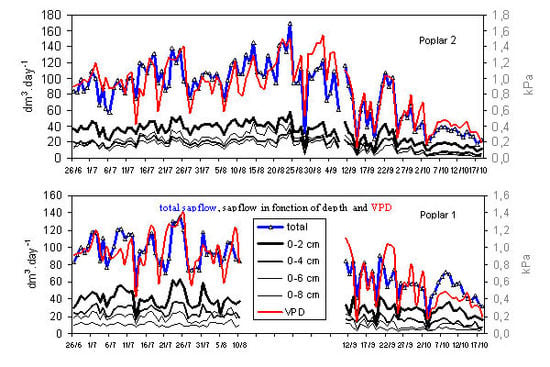
Following electronic problems with the probes some data were missing in the first poplar tree (P1) between mid-August and mid-September. However, results were comparable between the two poplar trees P1 and P2 over 84 days, i.e., almost three months (Figure 1). Measurements in P1 showed a steady decrease in the mean daily Qsi from the outer to inner depth; i.e., from 24.9 dm³ dm^–2 day^–1 at 0–2 cm to 13.5 dm³ dm^–2 day^–1 at 6–8 cm (Table 1). In P2, sap flows were more homogeneous and slightly lower, except in the inner 6–8 cm. From one day to another, very high daily variations in Qsi could be observed, with possible sharp drops or increases from one day to another. Maximum Qsi values were as high as 10 to 15 times the minimum. The mean values of the Qsi were 18.6 and 15.7 dm³ dm^–2 day^–1 in P1 and P2, respectively.

Figure 1. Daily variation of sap flux density (Qsi) in the two I214 poplars.

Figure 1. Daily variation of sap flux density (Qsi) in the two I214 poplars.

Table 1. Radial patterns of sap flow for the two I214 poplars (n = 84 days).

P1						P2
	0-2cm	2-4cm	4-6cm	6-8cm	0-8cm		0-2cm	2-4cm	4-6cm	6-8cm	0-8cm
Qsi sap flux density (dm3 dm−2 day−1)					mean Qsi	Qsi sap flux density (dm3.dm−2.day−1)					mean Qsi
mean	24.9	18.4	17.6	13.5	18.6	mean	19.1	12.2	16.2	15.2	15.7
sd	8.2	6.9	7.8	5.0	7.0	sd	7.54	5.14	8.43	7.68	7.2
min	6.3	4.3	3.7	3.4	4.4	min	3.31	2.54	2.32	2.19	2.6
max	45.4	32.7	33.5	25.3	34.2	max	33.1	21.9	32.8	29.0	29.2
Qi sap flow (dm3.day−1)					total Q	Qi sap flow (dm3.day−1)					total Q
mean	35.7	21.3	15.6	8.6	81.3	mean	30.3	16.1	17.3	12.4	75.9
sd	11.2	7.4	6.8	3.1	25.6	sd	11.8	6.8	9.0	6.3	33.2
min	12.5	7.1	3.3	3.1	28.6	min	5.2	3.4	2.5	1.8	16.6
max	64.5	37.0	29.5	15.9	135.5	max	52.0	28.9	35.0	23.7	137.9
Pi, percentage of total sap flow Q (%)						Pi, percentage of total sap flow Q (%)
					total						total
mean	44.6	26.2	18.6	10.7	100.0	mean	41.1	21.6	21.7	15.6	100.0
sd	6.1	3.6	4.7	2.3	0.0	sd	5.7	3.17	3.37	2.41	0.0
min	27.9	16.3	7.7	6.3	100.0	min	24.5	16.8	13.8	9.82	100.0
max	59.8	34.7	32.5	17.0	100.0	max	57.1	43.1	26.1	21.03	100.0

Table 1. Radial patterns of sap flow for the two I214 poplars (n = 84 days).

P1						P2
	0-2cm	2-4cm	4-6cm	6-8cm	0-8cm		0-2cm	2-4cm	4-6cm	6-8cm	0-8cm
Qsi sap flux density (dm3 dm−2 day−1)					mean Qsi	Qsi sap flux density (dm3.dm−2.day−1)					mean Qsi
mean	24.9	18.4	17.6	13.5	18.6	mean	19.1	12.2	16.2	15.2	15.7
sd	8.2	6.9	7.8	5.0	7.0	sd	7.54	5.14	8.43	7.68	7.2
min	6.3	4.3	3.7	3.4	4.4	min	3.31	2.54	2.32	2.19	2.6
max	45.4	32.7	33.5	25.3	34.2	max	33.1	21.9	32.8	29.0	29.2
Qi sap flow (dm3.day−1)					total Q	Qi sap flow (dm3.day−1)					total Q
mean	35.7	21.3	15.6	8.6	81.3	mean	30.3	16.1	17.3	12.4	75.9
sd	11.2	7.4	6.8	3.1	25.6	sd	11.8	6.8	9.0	6.3	33.2
min	12.5	7.1	3.3	3.1	28.6	min	5.2	3.4	2.5	1.8	16.6
max	64.5	37.0	29.5	15.9	135.5	max	52.0	28.9	35.0	23.7	137.9
Pi, percentage of total sap flow Q (%)						Pi, percentage of total sap flow Q (%)
					total						total
mean	44.6	26.2	18.6	10.7	100.0	mean	41.1	21.6	21.7	15.6	100.0
sd	6.1	3.6	4.7	2.3	0.0	sd	5.7	3.17	3.37	2.41	0.0
min	27.9	16.3	7.7	6.3	100.0	min	24.5	16.8	13.8	9.82	100.0
max	59.8	34.7	32.5	17.0	100.0	max	57.1	43.1	26.1	21.03	100.0

Once the sap flux densities Qsi are weighted at each depth by the annular areas of the corresponding sapwood using Equation 1 (Section 3.2.), the resulting sap flow Qi provides the daily water uptake by the tree at each radial depth (Table 1). In P1 sapwood areas at the four increasing depths were 1.38, 1.13, 0.88, 0.63 dm² respectively (total = 4.02 dm² over 0–8 cm). In P2, sapwood areas were 1.57, 1.32, 1.07 and 0.82 dm² with a total of 4.78 dm² over 0–8 cm.

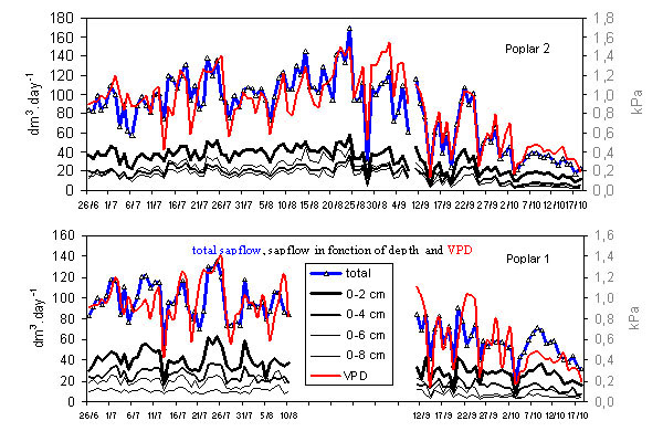
In P1, there was a steady decreasing trend in the mean Qi values from the outer to inner sapwood (i.e., from 35.7 dm³ day^–1 at 0–2 cm to 8.6 dm³ day^–1 at 6–8 cm), with again sharply contrasts from one day to another (Figure 2). In P2, sap flows were less contrasted (i.e., from 30.0 dm³ day^–1 at 0–2 cm to 12.4 dm³ day^–1 at 6–8 cm).

Figure 2. Daily variation of sap flow Qi at the four radial depths and at the tree level (Q) for the two I214 poplars with the corresponding daily vapor pressure deficits (VPD).

Figure 2. Daily variation of sap flow Qi at the four radial depths and at the tree level (Q) for the two I214 poplars with the corresponding daily vapor pressure deficits (VPD).

2.2. Variation in water use

At the tree level, the daily whole tree water use Q were computed as the sum of the Qi over the four depths (i.e. over 0–8 cm) using Equation 2 (Section 3.2.). Thus, over a period of 84 days, the daily tree water use fluctuated in the range of 28.6 to 135 dm³ day^–1 in P1 and 16.6 to137.9 dm³ day^–1 in P2, with an overall mean daily total of 81.3 dm³ day^–1 and 75.9 dm³ day^–1, respectively. In both trees, 41 to 45% of the total sap was flowing in the outer 0–2 cm ring. In contrast, the contributions of the other three depths remained between 19 and 26% at 2–4 cm and 4–6 cm, and close to 10 to 15% at the inner depth of 6–8 cm. This decreasing contribution is due to both decreasing sap flux densities and decreasing areas of sapwood with increasing depths. Results also indicates that in P2, the internal sap flow (4–8 cm) was relatively higher than in P2 and represented about 37 % of the whole tree water use compared to 29 % in the P1 (Table 1). Results also showed that despite the very high fluctuation of sap flow and whole tree water use from one day to another, contributions of each sapwood depth to the total water uptake did not fluctuate so much and remained rather stable, as indicated by relatively low standard deviations from 2.3 to 6.1 % (Table 1). In other words, an increase (or decrease) in water uptake by a tree is done by a simultaneous and proportional increase (or decrease) in sap flow at all depth.

2.3. Estimating water use

As the contribution of each sapwood depth remained rather stable and in order to avoid excessive number of probes in measurement campaigns, it was interesting to verify how far sap flux densities Qsi measured by a single probe, inserted in the most external (and active) wood depth (0–2 cm), could be used as a good estimator of the whole tree water use Q. Linear models of regressions computed over 84 days of measurements were y = 3.17 x (R2 = 0.88) and y = 4.02 x (R2 = 0.96) in P1 and P2, respectively (Figure 3). 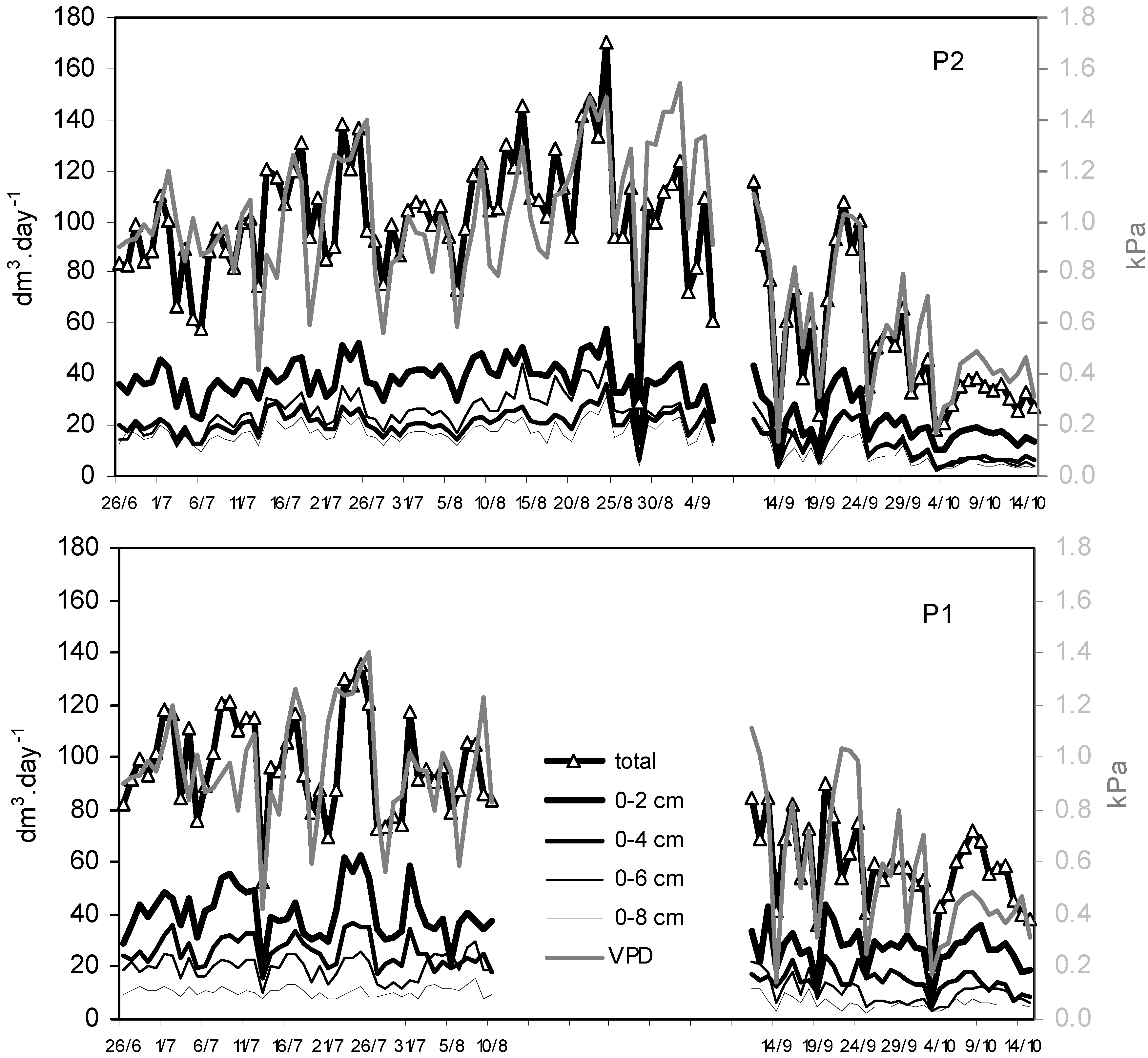In P2, the linear regression could be computed over 111 days and provided almost the same model (y = 4.15 x, R²=0.95) as over 84 days, indicating the strength of the model. When data are normalized according to a standard stem radius of 25 cm, corresponding slopes of regressions would be closer, with 3.30 and 3.70 for P1 and P2 respectively (n = 84 days). Another modeling issue was to see if environmental data could be considered as good regressors for estimating the whole tree water use. Unfortunately, data acquired in an official meteorological station located 5 km apart gave very poor modeling results with temperature, air humidity, corresponding vapor pressure deficit (VPD) and potential evapotranspiration data (PET). However, VPD computed from air temperature and humidity acquired in the plantation plot at the same rate than the sap flow data was a good regressor. Over 84 days, the linear regression model was y = 69.5 x + 25.5 (R2 = 0.67) with P1, and y = 97.6 x (R2 = 0.78) with P2 (Figure 4). The model remained stable over 111 days with P2 (y = 95.8 x; R2 = 0.76). This indicates that in a floodplain forest the micro climate is different from the nearby agricultural lands on the fluvial terraces, and that transpiration of trees responds better to environmental variables which are collected in situ.

The residual errors on water use were 9 dm³ day^–1 and 6 dm³ day^–1 for regression models based on sap flow measurements at 0–2 cm, and were 20 and 14 dm³ day^–1 for models based on the VPD, in P1 and P2, respectively. The Durbin–Watson test was used to verify the independence of the errors (absence of correlation between the daily values throughout the season). The D-values obtained over 84 days ranged from 1.82 to 2.16 in P1 and from 1.47 to 2.04 in P2. Possible D-values may range between 0 (a highly negative correlation) and 4 (a highly positive correlation), while a D-value of 2 corresponds to a correlation of 0.

Figure 3. Linear regressions of the whole tree water use (Q) on the sap flux density (Qsi) at the 0-2 cm depth (n=84 days).

Figure 3. Linear regressions of the whole tree water use (Q) on the sap flux density (Qsi) at the 0-2 cm depth (n=84 days).

Qsi (dm³ dm^–2 day^–1)

Figure 4. Linear regressions of the whole tree water use (Q) on the vapor pressure deficit (n=84 days).

Figure 4. Linear regressions of the whole tree water use (Q) on the vapor pressure deficit (n=84 days).

2.4. Discussion

Poplars in this plot were planted at a regular interval of about 7 m and each could explore an area of about 50 m². Considering the mean water table depths as a limiting factor for the root development (-3.54 m below P1 and -1.45 m below P2), the soil volumes available for the root systems were 3.54 * 50 = 177.0 m³ and 1.45 *50 = 72.5 m³, respectively (i.e., about 2.5 times more for P1 than for P2). During the first 7 years of growth, the P2 poplar grew slightly quicker than P1. P2 and the 8 surrounding trees had a mean trunk diameter of 27.1 cm, whereas the corresponding poplars with P1 had a mean diameter of 24.1 cm. The mean difference in diameter was 3 cm but was not significant. Water extraction from the soil by P1 necessitates a more developed root system, which is probably developed in the early years of the tree at the expense of a less developed aerial system. Water use by P1 seemed to be slightly higher than by P2, however the significance of this result cannot be stated as no replicates were done. Three years later, new measurements on the stem diameters revealed that P1 and the 8 neighbor trees were growing quicker (+28%) than around P2 (+23%), and the mean difference in diameter was reduced. These results were not really surprising as poplars are known to be able to better extract soil moisture from unsaturated zones than Salix species, even when groundwater is available [15]. Such ability was also confirmed by isotopic measurements made on the same trees of this study [16].

This study also showed that a difference in water table level (all other factors being equal) could probably induce a modification in the radial sap flow profile of poplars and in the water use. When the water table was close to the surface, the radial sap flow profile in the stem seemed to be more stable and more homogeneous and the models stronger. When the water table was lower, the sap flow was more important in the outer tree rings and showed a higher radial variability. In very dry conditions the sapwood is less developed and tree rings are narrower as observed on native black poplars [17].

At the whole tree level, water use was highly fluctuating from one day to the other (minimum 17 dm³ day^–1; maximum 138 dm³ day^–1) but could be rather well correlated to the local VPD, a result consistent with a study on the tremble aspen, P. tremuloides Michx. [18]. In P1, the quality of the regression model with the VPD was slightly lower than with P2 but in this case, a 3.5 m deep water table was apparently not a limiting factor for the uptake of water by the trees, as no thick gravel bar hindered water uptake in the soil profiles. It can be noted that by forcing the regression model to pass by the origin, rather than to try to obtain the best R² coefficient, the new model for P1 is actually very similar to P2 model, with y = 97.891 (R2 = 0.54). As a rule of thumb one may consider water use (in dm³ day^–1) ~ 100 * VPD (in kPa). However, this should be confirmed by other measurements especially during stress or drought periods.

Despite very high daily fluctuations in sap flows, and regardless of how low the sap flow might be (e.g., presence of clouds or leaf fall at the end of the season), each xylem depth maintained a rather stable contribution to the whole tree water use Q (e.g., 40 to 45% in the outer two first centimeters of the stems). This indicates that once the sap flow radial pattern of a poplar tree is known, following an initial preliminary test over several weeks, it should be possible to restrict sap flow measurements to the outer 0–2 cm for long term measurements and to compute the total daily uptake using the regression models (e.g., in this study Q ~ 4.0 * Qsi with P2 and Q ~ 3.2 * Qsi with P1, or for a standard tree of 25 cm, DBH, Q ~ 3.5 * Qsi). However, it is of great importance to check in further studies whether sap flow radial patterns, as observed over one vegetative season, remain similar from one year to another and at different tree age, and if sap flow is still active beyond a depth of 8 cm (although existing probes are not yet manufactured to reach such depths). By ignoring the activity of more internal sapwood there is a risk of underestimating the actual water uptake. This error is limited because both sap flow and sapwood area decrease with depth in the stem. If one assumes that at 8–10 cm sap flow remained the same as at 6–8 cm, corrections of water use at the tree level would be, as a maximum, + 10 % with P1 and + 15 % with P2.

3. Experimental Section

3.1. Study site

The experimental site (43°49’ N, 1°15’ E, 98 m above sea level) was located in a 3 km wide floodplain of the Garonne River, 35 km downstream from the city of Toulouse, in the southwest of France. The mean annual discharge is 240 m³ s^–1, annual floods are close to 1400 m³ s^–1 and centennial floods are above 6500 m³ s^–1. During summer, the minimum flow is artificially sustained above 42 m³ s^–1 using water from reservoirs in the Pyrenees. The mean annual rainfall is 672 mm, 159 mm of which falls during the three summer months. The mean annual potential evapotranspiration is 894 mm, 421 mm of which occurs in summer. Therefore, each year the climatic summer deficit is about 260 mm.

A plantation of I214 hybrid poplars of the same age (seven years), the same genetic stock (clone I214) and the same life history (same farm practices since the trees were planted) was chosen near (and perpendicular to) the brook running along the foot of a Quaternary terrace, 600 m away from the riverbed (i.e., in the decennial floodplain). The dimension of the plantation was 200 m x 50 m with a density of 200 trunks ha^–1. The soil surface was sub-horizontal with maximum elevation differences of 50 cm between the two ends of the plot. Sap flow measurements were made in a first tree (P1) located in the second row of the poplar plantation (i.e., at a distance of 180 m from the brook) and in a second tree (P2) chosen in the second last row of the plot (i.e., 20 m from the brook). Tree heights were 19.5 and 20.7 m, respectively. P1 had a diameter of 24.0 cm and its eight neighboring trees diameters ranging from 22.9 to 25.5, with a mean value of 24.1 cm. P2 had a diameter of 27.1 cm and its eight neighboring trees diameters ranging from 25.4 to 29.8 cm, with a mean value of 27.1 cm. Corresponding basal areas were 9.1 m² ha^-1 and 11.5 m² ha^-1, respectively.

Observations on the water table were made using three piezometers during one year. Near the brook, close to P2, the mean water table depth was -1.45 m with a standard deviation sd = 0.16 m. In the middle of the plots (about 100 m from the brook), the mean water table depth was -2.96 m (sd = 0.47 m), while at the foot of P1, at the other end of the plot (180 m from the brook) the depth was -3.54 m (sd = 0.46 m). In this situation, the only apparent factor that could differentiate the two trees, which were separated by 160 m, was the stable vertical gradient of about 2 m in the water table depth. Soils extracted for the boring of the piezometers were similar and revealed that the Fluviosols had an Holocene origin with alternating layers of sand, sandy silt and silt up to 4 m. Beyond a depth of 4 m, coarse deposits with dominant gravels were observed in P1 and with the Tertiary impermeable ‘molasses’ substrate in P2. Thus, the two trees were located in the two most contrasting sites within the plantation. Under the trees, there was no understory, as the farmer used to plough once or twice a year to avoid competition between herbaceous and the trees and to favor a better penetration of rains in the soil.

3.2. Sap flux measurements

Sap flux were measured using 2 cm Granier probes [19] at four increasing radial depths (0–2, 2–4, 4–6 and 6–8 cm) in both trees. This limit of 8 cm was imposed by the fact that probes are not presently manufactured for measurements beyond 8 cm. However, this maximum depth was consistent with the hydraulic conductivity measurements made in poplar trees by Edwards and Booker [3], indicating that the mean conductivity at 1 cm increments decreased with radial depth and was close to zero at 8 cm.

The four probes were positioned within the same quadrant of the tree and faced north to avoid thermal interference from the sun. They were isolated and protected behind a Trisodur material, in which four reflective aluminum foils alternate with three thermo-insulator Dacron layers. Measurements were made every 30 s over four months (26 June–18 October). Data were then averaged and recorded every 5 minutes in dataloggers. Sap flux density Qsi at the depths i, (with i = 1 to 4 for measurements at 0–2, 2–4, 4–6 and 6–8 cm, respectively) was expressed in dm³ of sap per dm² of sapwood area per day (dm³ dm^–2 day^–1).

The sapf flow Qi at the depths i, was computed in dm³ day^–1 by weighting each sap flux density Qsi by the corresponding sapwood area Ai :

Qi = Ai * Qsi

(1)

The daily whole tree water use, Q, was estimated, in dm³ day^–1, as the sum of the sap flows:

Q = ∑i Qi = ∑i (Ai * Qsi)

(2)

For estimating the variability of the contribution of each 2 cm sapwood ring to the total sap flow at the tree level, percentages of total sap flow were computed at each radial depth i as:

Pi= 100 * (Qi / Q) = 100 * (Qi / ∑i Qi).

(3)

4. Conclusions

This study provides indication on the range of variation in water use which exists in a homogeneous plantation of I214 poplars. Over 84 days, there is a factor of eight in the water use variation from one day to another, compared to only a mean difference of 7% between two “identical” trees. Such information was highly requested by the local farmers. Despite very high daily fluctuations in sap flows, and regardless of how low the sap flow might be (e.g., presence of clouds or leaf fall at the end of the season), each xylem depth maintained a rather stable contribution to the whole tree water use Q (e.g., 40 to 45% in the outer two first centimeters of the stems). This indicates that in such a situation, once the sap flow radial pattern of a poplar tree is known, following an initial preliminary test over several weeks, it should be possible to restrict sap flow measurements to the outer 0–2 cm for long term measurements and to compute the total daily uptake using the regression models. However, in large trees, sap flow may exist beyond a radial depth of 8 cm and a correction factor of +10 to +15 % on water use was suggested. In this study, the mean daily water use (computed over 84 days) corresponds roughly to 3.1 liter per day and per centimeter of DBH. With the correction factor, it makes ~ 3.5 liters day^-1 cm^-1 or 90 liters per day per tree. At the plantation level, if one neglects all other factors, the transpiration of poplars represents a mean water uptake of 18 m³ ha^-1day^-1 or 1.8 mm day^-1.

References and Notes

1. Stettler, R.F.; Bradshaw, H.D., Jr.; Heilman, P.E.; Hinckley, T.M. Biology of Populus and its implications for management and conservation; NRC Research Press: Ottawa, Canada, 1996; pp. ix–xi. [Google Scholar]
2. FAO. Peupliers et Saules; Collection FAO forêts N°10; UN-FAO: Rome (Italy), 1980; pp. 11–46. [Google Scholar]
3. Edwards, W.R.N.; Booker, R.E. Radial variation in the axial conductivity of Populus and its significance in heat pulse velocity measurement. J. Exp. Bot. 1984, 35, 551–561. [Google Scholar] [CrossRef]
4. Hinckley, T.M.; Brooks, J.R.; Čermák, J.; Ceulemans, R.; Kučera, J.; Meinzer, F.C.; Roberts, D.A. Water flux in a hybrid poplar stand. Tree Physiol. 1994, 14, 1005–1018. [Google Scholar] [CrossRef]
5. Hall, R.L.; Allen, S.J.; Rosier, P.T.W.; Hopkins, R. Transpiration from coppiced poplar and willow measured using sap-flow methods. Agr. Forest Meteorol. 1998, 90, 275–290. [Google Scholar] [CrossRef]
6. Meiresonne, L.; Nadezhdina, N.; Čermák, J.; Van Slycken, J.; Ceulemans, R. Measured sap flow and simulated transpiration from a poplar stand in Flanders (Belgium). Agr. Forest Meteorol. 1999, 96, 165–179. [Google Scholar] [CrossRef]
7. Phillips, N.; Oren, R.; Zimmerman, R. Radial patterns of xylem sap flow in non-, diffuse- and ring-porous tree species. Plant Cell Environ. 1996, 19, 983–990. [Google Scholar] [CrossRef]
8. Guevara-Escobar, A.; Edwards, W.R.N.; Morton, R.H.; Kemp, P.D.; Mackay, A.D. Tree water use and rainfall partitioning in a mature poplar-pasture system. Tree Physiol. 2000, 20, 97–106. [Google Scholar] [CrossRef] [PubMed]
9. Nadezhdina, N.; Čermák, J.; Ceulemans, R. Radial patterns of sap flow in woody stems of dominant and understory species: scaling errors associated with positioning of sensors. Tree Physiol. 2003, 22, 907–918. [Google Scholar] [CrossRef]
10. Hatton, T.J.; Moore, S.J.; Reece, P.H. Estimation stand transpiration in a Eucalyptus populnea woodland with the heat pulse method: measurement errors and sampling strategies. Tree Physiol. 1995, 15, 219–227. [Google Scholar] [CrossRef] [PubMed]
11. Schaeffer, S.M.; Williams, D.G.; Goodrich, D.C. Transpiration of cottonwood/willow forest estimated from flux. Agr. For. Meteorol. 2000, 105, 257–270. [Google Scholar] [CrossRef]
12. Wullschleger, S.D.; King, A.W. Radial variation in sap velocity as a function of stem diameter and sapwood thickness in yellow-poplar trees. Tree Physiol. 2000, 20, 511–518. [Google Scholar] [CrossRef] [PubMed]
13. Lambs, L.; Muller, E. Sap flow and water transfer in the Garonne River riparian woodland, France: first results on poplar and willow. Ann. For. Sci. 2002, 59, 301–315. [Google Scholar] [CrossRef] [Green Version]
14. Zhang, H.; Morison, J.I.L.; Simmonds, L.P. Transpiration and water relations of poplar trees growing close to the water table. Tree Physiol. 1999, 19, 563–573. [Google Scholar] [CrossRef] [PubMed]
15. McQueen, I.S.; Miller, R.P. Soil moisture and energy relationships associated with riparian vegetation near San Carlos, Arizona, Gila River phreatophyte project; Geological Survey professional paper 655-E; USGS: Washington DC, USA, 1972; pp. 5–15. [Google Scholar]
16. Lambs, L.; Loudes, J.P.; Berthelot, M. The use of the stable oxygen isotope (18O) to trace the distribution and uptake of water in riparian woodlands. Nukleonika 2002, 47, 71–74. [Google Scholar]
17. Lambs, L.; Loubiat, M.; Girel, J.; Tissier, J.; Peltier, J-P.; Marigo, G. Survival and adaptation of Populus nigra to drier conditions after damming of an alpine river, southeast France. Ann. For. Sci. 2006, 63, 377–385. [Google Scholar] [CrossRef]
18. Hogg, E.H.; Hurdle, P.A. Sap flow in trembling aspen: implication for stomatal responses to vapor pressure deficit. Tree Physiol. 1997, 17, 501–509. [Google Scholar] [PubMed]
19. Granier, A. A new method to measure the raw sap flux in the trunk of trees. Ann. For. Sci. 1985, 42, 193–200. [Google Scholar] [CrossRef]