A Hydraulic Friction Model for One-Dimensional Unsteady Channel Flows with Experimental Demonstration

Abstract

As a critical parameter of the steady uniform friction model, the roughness coefficient changes with flow unsteadiness in flood events; i.e., the flow conditions of the stream segment significantly affect the flow resistance. In this study, a modified formula was established to improve the unsteady friction simulation; ten terms relating to the first- and second-order time and space partial derivatives of hydraulic parameters were selected as additional terms. The results of a hydraulic experiment show that the hysteresis between flow depth and mean cross-sectional velocity cannot be neglected in unsteady flows that disturb the performance of a steady uniform friction model. Six terms have a strong correlation with objective friction. Further, three of them have a small variance in correlation coefficient. Then, the composition of the proposed formula was determined. The results show that adding too many additional terms provides better performance in the calibration phase, yet reduces the accuracy of the validation phase because of an overfitting phenomenon. The optimal number of additional terms is three, and the established formula can improve the unsteady friction simulation.

1. Introduction

As the foundation of many hydraulic models and basic hydraulics theories, one-dimensional (1D) unsteady flow resistance in open-channel flows has been widely studied [1,2]. Although it is difficult to establish a comprehensive mathematical model for the 1D unsteady flow resistances in a channel due to the complexity of unsteady flow conditions, many studies have dealt with the problem as an inverse problem of the momentum equation of Saint-Venant equations [3,4]. A significant difference was observed between steady uniform and unsteady frictions. For example, Mrokowska et al. reported that the steady-state formula for frictional slope and shear velocity is not applicable to unsteady flow [5]. Fread reported that the trend of Manning coefficient vs. flow rate decreases when the inundation area is relatively small compared to an in-bank flow area, or increases in the reversed case, indicating that the Manning coefficient is a misleading parameter to investigate the relationship between resistance and flow rate [6]. For the terms in the momentum equation of Saint-Venant equations, Zhou and Graf found that the temporal and spatial derivatives of flow depth and mean cross-sectional velocity significantly affect the frictional resistance of a dynamic wave, indicating that more factors affect unsteady flow resistance compared with steady flow [7].

Hydraulic experiments have been designed to investigate the characteristics of unsteady flows as well as unsteady friction and shear stress [8,9]. For example, Sutter et al. reported that the capacity of sediment transport increases when the unsteadiness of flow increases; this can be considered as the result of the effect of flow unsteadiness on shear stress [10]. Further, in unsteady flows, a hysteresis effect was detected; a phase lag was observed between flow depth and mean cross-sectional velocity peaks [3,5]. The hysteresis effect results in different characteristics of flow resistance in the rising and falling limbs of a hydrograph [11]. This indicates that most steady uniform friction algorithms or quasi-steady friction algorithms based on the kinematic wave approximation have limited practical implications, as most natural flood waves are noninertial with close instantaneous and local wave crests [12]. Bombar reported that a more unsteady hydrograph was correlated with increased hysteresis in the hysteretic behavior [9].

Despite these achievements in clarifying the difference between steady uniform and unsteady friction, many studies have focused on measuring the unsteady flow resistance indirectly using algorithms or simplified algorithms based on the momentum equation of Saint-Venant equations instead of exploring an empirical friction formula that can be applied to unsteady flows. Besides, although some methods are available to calculate the flow resistance in two-dimensional (2D) flows (e.g., the method based on the Reynolds equation, which takes the advantage of theoretical relationships between shear stress and horizontal velocity distribution), they require turbulent information which is unavailable in a 1D problem [3,13]. Therefore, in a 1D hydrodynamic model comprising Saint-Venant equations and a 1D empirical friction model, 1D steady uniform friction models (e.g., Chezy formula, Manning formula, and Darcy–Weisbach friction formula [14]) are still used for unsteady friction simulation [15], often leading to large errors [16,17].

Real-time roughness updating methods are used for 1D hydrodynamic models to update the roughness coefficient dynamically [18]. For example, the discharge and stage of adjacent up- and down-sections were used for the dynamic correction of roughness [19]. Using the Gauss–Newton methods, a roughness updating model was developed to minimize the error in stage forecast [20]. Based on Kalman filter, the roughness coefficient was updated in flood forecast [21]. An optimum solution method was used to identify the inverse problem of roughness parameter [22]. Although these approaches improve the unsteady friction simulation accuracy to some extent and indicate the inapplicability of steady uniform friction formula in unsteady flows, these studies are based on a classical steady uniform friction model. The roughness coefficient must be updated quickly to achieve an accurate friction. The physical interpretation of roughness coefficient is distorted, hindering further application in hydraulic forecasting.

An empirical friction formula that can be applied to an unsteady flow is urgently needed. Based on the results of a previous study, flow resistance is relevant to both the boundary characteristics of a channel and flow conditions of a stream segment [23]. The roughness coefficient is used to quantify the boundary characteristics of a channel [24]; it is related to the cross-section shape, grain-size distribution, and submerged aquatic plants [25]. Mean cross-sectional velocity, flow depth, and Reynolds number are used to describe the flow conditions of a stream segment in a 1D steady uniform friction model [24]. In the case of an unsteady flow, the flow conditions of a stream segment are more complex than those of a steady uniform flow. Its motion parameters (i.e., mean cross-sectional velocity and flow depth) are time-varying and nonuniform in the stream-wise direction. These factors affect the magnitude of friction force [7].

This study aims to analyze the differences between unsteady and steady uniform frictions, especially the effects of nonuniformity and unsteadiness on friction magnitude. The first- and second-order derivatives of motion parameters were selected as additional terms and added to a linear modified friction formula to achieve a better performance in unsteady flow. The optimal number of additional terms was determined using the hydraulic flume experimental data. Moreover, a modified formula was established to improve the unsteady friction simulation.

2. Materials and Methods

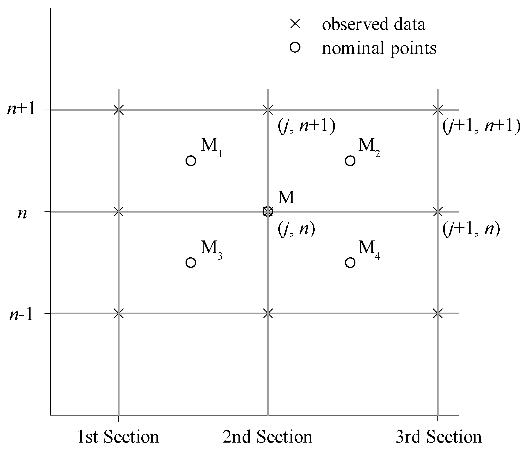
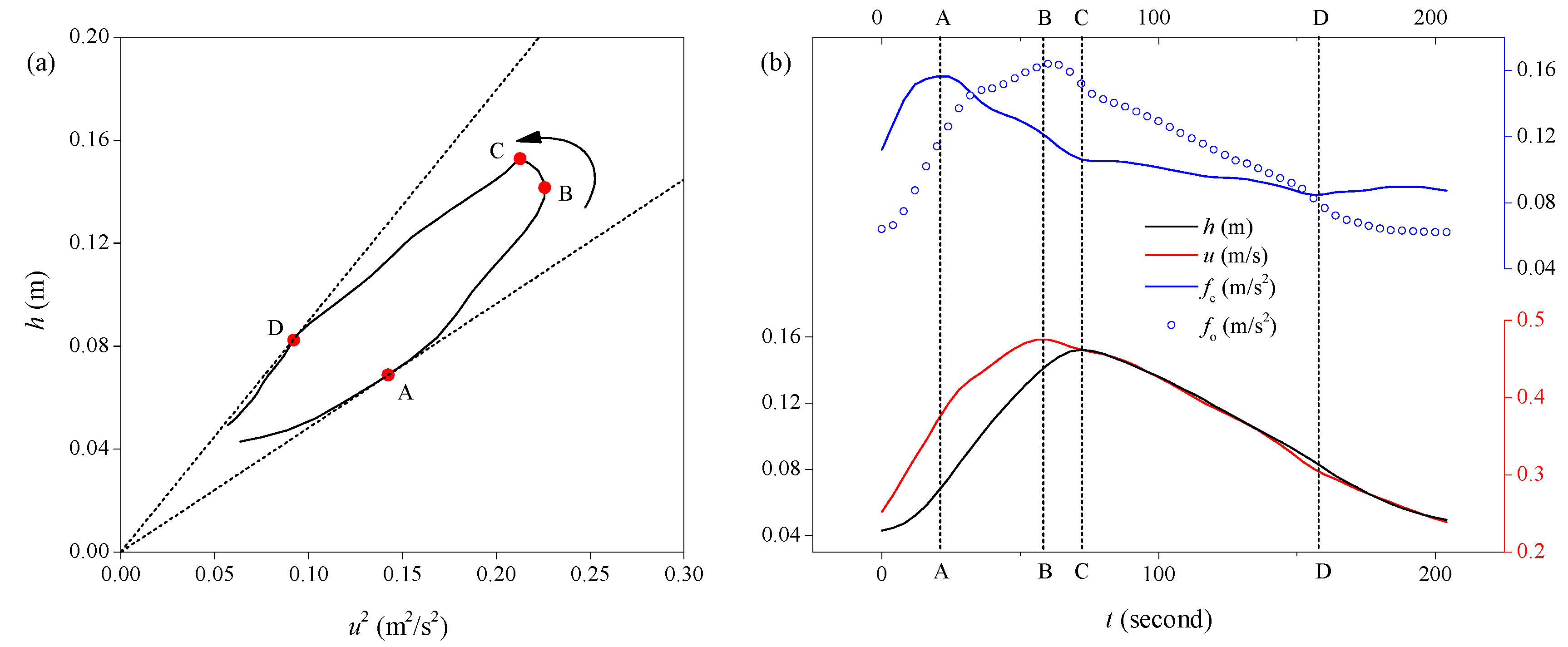
2.1. Analysis of Unsteady Friction

A 1D hydraulic friction model for an unsteady channel flow was used to generalize the flow resistance at the stream segment. Except for liquid properties, flow resistance is relevant to both the boundary characteristics of channel and flow conditions of the stream segment. In the derivation of steady uniform friction formulas, the relevant hydraulic parameters are density, dynamic viscosity, hydraulic radius, relative roughness, flow depth, and mean cross-sectional velocity [26]. The most significant difference between unsteady and steady uniform flows is that the flow conditions in an unsteady flow have nonuniformity and unsteadiness. The partial derivatives of hydraulic parameters are the most relevant physical variables to describe flow unsteadiness and flow nonuniformity in 1D problems [5]. The dependence of unsteady flow resistance on derivatives (e.g., ∂u/∂t, ∂u/∂x, and ∂h/∂x) is significant [1,2]. Sometimes, the roughness coefficient can be expressed as a function of derivative ∂h/∂t [7]. Therefore, in this study, the first- and second-order time and space partial derivatives of hydraulic parameters (i.e., mean cross-sectional velocity and flow depth) were selected to characterize the nonuniformity and unsteadiness of the channel flow. Thus, the frictional resistance of a unit volume of water is a function of these factors and can be expressed as follows:

$$F/(Al)=\Psi \left(\rho ,\mu ,R,\frac{k}{R},h,u,\frac{\partial h}{\partial t},\frac{\partial h}{\partial x},\frac{\partial u}{\partial t},\frac{{\partial }^{2}h}{\partial t^2},\frac{{\partial }^{2}h}{\partial t\partial x},\frac{{\partial }^{2}h}{\partial x^2},\frac{{\partial }^{2}u}{\partial t^2},\frac{{\partial }^{2}u}{\partial t\partial x},\frac{{\partial }^{2}u}{\partial x^2}\right)$$

(1)

where F is the frictional resistance, A is the cross-sectional area, l is the length of the stream segment, F/Al is the friction of a unit volume of water, ρ is the water density, μ is the dynamic viscosity, h is the flow depth, u is the mean cross-sectional velocity, k/R is the relative roughness where k is the mean roughness height, R is the hydraulic radius, and the other items are the first- and second-order time and space partial derivatives of h and u.

In a wide shallow channel, R is approximated to h [27]. However, the implication of this approximation is more complex in unsteady flow; i.e., many friction models are established based on the kinematic wave concept, and the hysteresis between flow depth and mean cross-sectional velocity is neglected. The difference between R and h clearly affects the simulation results. However, this study involves unsteady flows without a kinematic wave approximation. In the case of a nonkinematic wave, the hysteresis between flow depth and mean cross-sectional velocity cannot be neglected. The phase difference between h and u inadvertently disturbs the simulation result when the steady uniform frictional formula is applied to unsteady flow. This is an unexpected model structure error, which was fully analyzed in this study. Further, because of the one-to-one relationship between h and R, there is no difference between the use of h and R when considering this unexpected model structure error. Therefore, R was approximated to h in this study. Then, in the dimensional analysis, h, u, and ρ were selected as the fundamental dimensions. In the case of channels/natural rivers, the river bed is irregular, flanked by sand dunes and indigenous plants. The relationships between friction factor and Reynolds number depend on many irregularity factors. The friction factors mentioned in this paper as well as traditional friction factors like Chezy’s coefficient C and Manning’s roughness coefficient n are regarded as empirical parameters independent of Re [28]. Hence, Re was neglected during the dimensional analysis. The following dimensionless relationship was derived by applying Π theory [26].

$$f/(\frac{u^2}{h})=\Psi \left(\frac{k}{h},\frac{1}{u}\frac{\partial h}{\partial t},\frac{\partial h}{\partial x},\frac{h}{u^2}\frac{\partial u}{\partial t},\frac{h}{u}\frac{\partial u}{\partial x},\frac{h}{u^2}\frac{{\partial }^{2}h}{{\partial }^{2}t},\frac{h}{u}\frac{{\partial }^{2}h}{\partial t\partial x},h\frac{{\partial }^{2}h}{\partial x^2},\frac{h^2}{u^3}\frac{{\partial }^{2}u}{\partial t^2},\frac{h^2}{u^2}\frac{{\partial }^{2}u}{\partial t\partial x},\frac{h^2}{u}\frac{{\partial }^{2}u}{\partial x^2}\right)$$

(2)

where f = F/ρAl is the friction of the unit mass of water.

The above equation shows that friction can be generalized as a function related to the boundary characteristics of channel and flow conditions of the stream segment. In addition, according to the physical interpretation, a physical concept was introduced to simplify Equation (2): the river-bed roughness causes friction, while the flow conditions of stream segment affect its magnitude. Thus, the physical variables in Equation (2) can be further generalized into two parts:

$$f={\phi }_1\times {\phi }_2\times \left(\frac{u^2}{h}\right)$$

(3)

$${\phi }_1={\Psi }_1\left(\frac{k}{h}\right)$$

(4)

$${\phi }_2={\Psi }_2\left(\frac{1}{u}\frac{\partial h}{\partial t},\frac{\partial h}{\partial x},\frac{h}{u^2}\frac{\partial u}{\partial t},\frac{h}{u}\frac{\partial u}{\partial x},\frac{h}{u^2}\frac{{\partial }^{2}h}{\partial t^2},\frac{h}{u}\frac{{\partial }^{2}h}{\partial t\partial x},h\frac{{\partial }^{2}h}{\partial x^2},\frac{h^2}{u^3}\frac{{\partial }^{2}u}{\partial t^2},\frac{h^2}{u^2}\frac{{\partial }^{2}u}{\partial t\partial x},\frac{h^2}{u}\frac{{\partial }^{2}u}{\partial x^2}\right)$$

(5)

where ϕ₁ is the function of the boundary characteristics of a channel, defined as the roughness coefficient in a steady uniform friction model. ϕ₂ × u²/h is the function of flow conditions of the stream segment referring to motion parameters (characterized by h and u) and their partial derivatives of time and space.

Equations (3)–(5) indicate that the 1D unsteady friction of an open-channel flow is not only related to the roughness coefficient, but also to flow unsteadiness and nonuniformity. If the 1D steady uniform friction model is applied to simulate the unsteady friction losses, ϕ₂ is neglected, and the roughness coefficient is affected by these factors. This makes the roughness coefficient depend on flow unsteadiness and change in the flood events. Linear models are an effective tool in the preliminary stage of complex problems, and can be used as a simplified scheme for tough problems. In a linear model, the effect of each factor on the outcome can be considered by weights. Linear models are flexible and work well for most purposes [29]. The factors involved in ϕ₂ are expressed as a linear function to consider the effect of motion parameters’ partial derivatives of time and space on unsteady friction. Besides, ϕ₁ is used to quantify the characteristics of a channel. In this study, ϕ₁ is expressed as a function of relative roughness, yet is related to many factors in a natural river such as the cross-section shape, grain-size distribution, and submerged aquatic plants. For practical use, it is evaluated as a constant empirical parameter [30]. Thus, Equations (3)–(5) can be expressed as follows:

$$\begin{array}{l}f=c_1\frac{u^2}{h}+c_2\frac{u}{h}\frac{\partial h}{\partial t}+c_3\frac{u^2}{h}\frac{\partial h}{\partial x}+c_4\frac{\partial u}{\partial t}+c_{5}u\frac{\partial u}{\partial x}+c_6\frac{{\partial }^{2}h}{\partial t^2}\\ +c_{7}u\frac{{\partial }^{2}h}{\partial t\partial x}+c_8{u}^2\frac{{\partial }^{2}h}{\partial x^2}+c_9\frac{h}{u}\frac{{\partial }^{2}u}{\partial t^2}+c_{10}h\frac{{\partial }^{2}u}{\partial t\partial x}+c_{11}hu\frac{{\partial }^{2}u}{\partial x^2}\end{array}$$

(6)

where term 1 is a steady uniform friction term and has the same structure as the Chezy formula—a steady uniform friction model. Other terms are additional terms to consider the effects of flow unsteadiness: The 2nd to 5th terms are additional terms for the first-order partial derivatives of time and space of h and u, and the 6th to 11th terms are additional terms for the second-order partial derivatives of time and space of h and u.

In this section, to solve the problem of the low accuracy and inapplicability of steady uniform friction models, the structure of a 1D unsteady friction model for channel flow was analyzed. However, the initial version of the modified model is superfluous. The number of additional terms is too great—a disadvantage for practical applications. Certain hydraulic tests are required. According to the experimental data, the dependence of unsteady friction on each additional term and the optimal composition of additional terms should be fully evaluated.

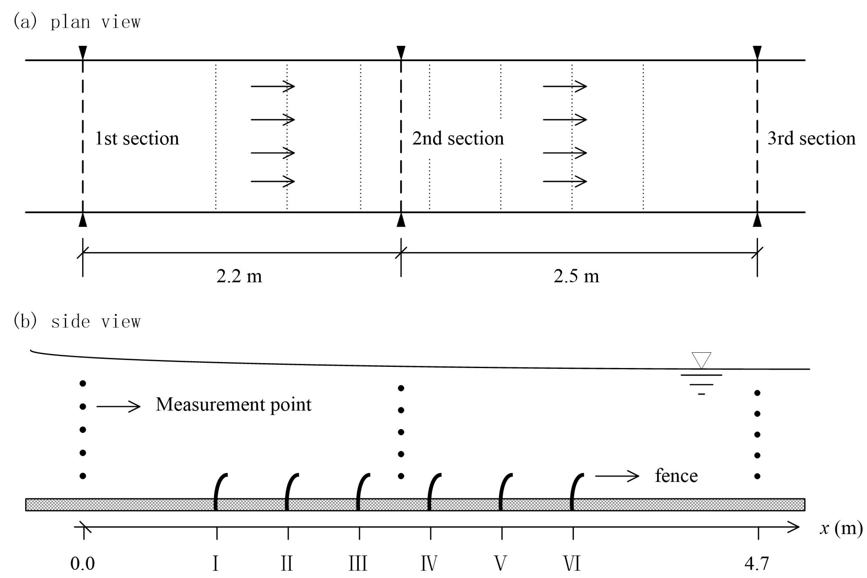
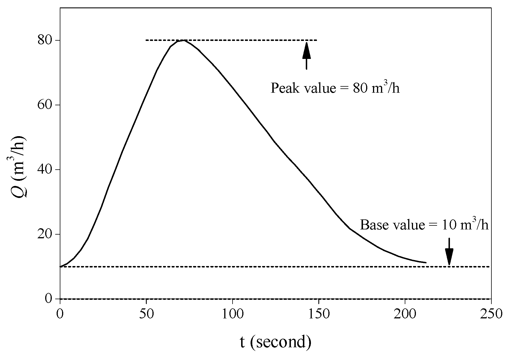
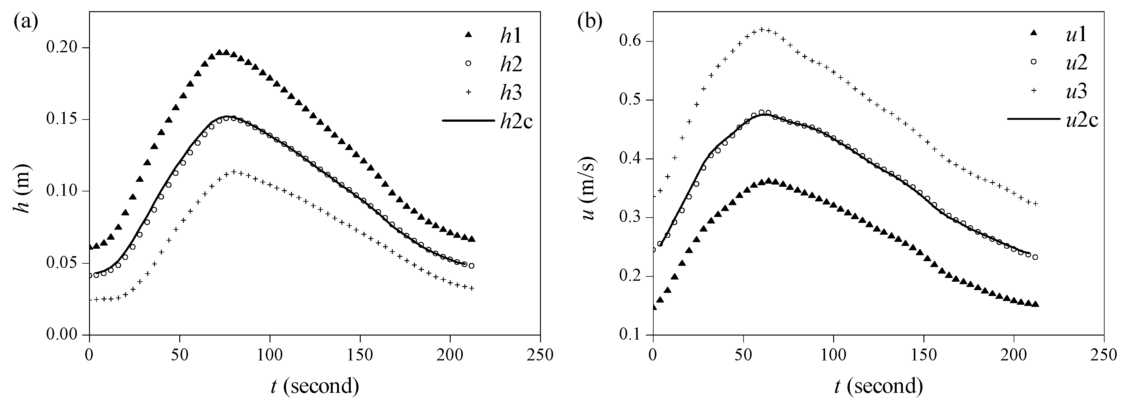
2.2. Experimental Procedure

Experiments were carried out in the Hydraulics laboratory of Hohai University. The experimental flume had a rectangular cross-section. Its length, width, and height were 8 m, 0.31 m, and 0.4 m, respectively. The flume was made of a smooth glass. Grains were placed at the flume bottom to imitate the roughness of river bed [31]. At the upstream of the flume, a water tank was set for straightening the incoming flow and eliminating large eddies. Vertical shutters were installed at the flume tail to stabilize the layer of bed material.

The flow depth and mean cross-sectional velocity were measured at three observation cross-sections (i.e., 1st, 2nd, and 3rd Sections) [7]. A length of 2.5 m upstream of the 1st Section was used to ensure that the velocity profile within the measuring reach was fully developed. The distance between each observation cross-section was carefully arranged so that the stage difference between two adjacent cross-sections was large enough to evaluate the spatial derivatives (e.g., ∂h/∂x and ∂²h/∂x²) accurately [4]. The distance between the 1st and 2nd Sections was 2.2 m, and that between the 2nd and 3rd Sections was 2.5 m as shown in Figure 1.

The effects of both the boundary characteristics and flow conditions of the stream segment were considered. The boundary characteristics of the flume were related to the cross-sectional shape, grain-size distribution, submerged aquatic plants, and many other factors. Equations (3)–(5) characterize them using the roughness coefficient—a comprehensive description of all these effects. In experiments, fences made of different numbers of plastic pillars were placed on the roughness bed to imitate river-bed conditions with different densities of aquatic plants [32]. Thirteen different modes of river-bed conditions were designed.

Table 1. Details of 13 different modes of river-bed conditions.

Experimental Mode	Fence Position
	I	II	III	IV	V	VI
Mode 1
Mode 2		1			1
Mode 3		2			2
Mode 4		3			3
Mode 5		4			4
Mode 6	1	1			1	1
Mode 7	2	2			2	2
Mode 8	3	3			3	3
Mode 9	4	4			4	4
Mode 10	1	1	1	1	1	1
Mode 11	2	2	2	2	2	2
Mode 12	3	3	3	3	3	3
Mode 13	4	4	4	4	4	4

shows the details; the schema index is numbered from 1 to 13. Mode 1 refers to no fence. From Modes 2 to 13, the larger the schema index number, the greater the roughness resistance from the fence. The fence index was numbered from 1 to 4; a larger fence index meant a higher plastic pillar density. Fences were placed at places numbered from I to VI: 0.9, 1.4, 1.9, 2.4, 2.9, and 3.4 m distance away from the 1st Section, respectively (Figure 1).

The flow conditions of a stream segment in a 1D unsteady friction model are related to the mean cross-sectional velocity, flow depth, Reynolds number, flow unsteadiness, and flow nonuniformity. According to Equations (3)–(5), flow unsteadiness and flow nonuniformity should be emphatically considered in the case of unsteady flows. Thus, in experiments, the discharge of incoming flow was changed from a base value to a peak value and then returned to the base value to simulate flood events with a single-peak hydrograph; the mean cross-sectional velocity and flow depth at each observed section changed with time and space [2,7]. An ultrasonic flowmeter installed in the inlet pipe was used to measure the discharge of incoming flow [2,9]. Three ranges of discharge (i.e., 10–60, 10–80, and 10–100 m³/h) were selected as Exps. 1, 2, and 3, respectively, to simulate flood events with different flow unsteadiness in each river-bed condition mode. Thus, 39 experiments were carried out. Figure 2 shows an example of the evolution of discharge at flume entrance.

The depth of water at each section was measured using a length gauge. An acoustic Doppler velocimeter (Vectrino II) was used to measure the point velocities at three sections. Vectrino II measures a velocity profile within a sampled water column of 35 mm with a resolution of 1 mm. Additionally, the velocity measurements were repeated five times at different relative depths [9]. Many procedures are used to obtain the time-varying mean of unsteady flow; e.g., Savitzky–Golay filter, Fourier transform, and moving average [4]. In this study, moving average was used because it is simple to use, yet provides good approximations [33].

$$\overline{u}\left(t\right)=\frac{1}{2\mathrm{N}+1}{\displaystyle \sum _{k=-\mathrm{N}}^{\mathrm{N}}u\left(t-k\right)}$$

(7)

where 2N + 1 is the number of data used to calculate the smoothed velocity $\overline{u}\left(t\right)$ from raw velocity time series u(t).

Then, a difference quotient method was used to obtain each term in Equation (6). A four-point quotient was used to evaluate the time and space derivatives at a nominal point M [4]. The corresponding four-point weighted average method was used to evaluate the variables at point M. The difference quotient method can be expressed as follows:

$$g{|}_{\mathrm{M}}=\psi \left[\theta g_{j+1}^{n+1}+\left(1-\theta \right)g_{j+1}^n\right]+\left(1-\psi \right)\left[\theta g_j^{n+1}+\left(1-\theta \right)g_j^n\right]$$

(8)

$$\frac{\partial g}{\partial x}{|}_{\mathrm{M}}=\frac{\theta \left(g_{j+1}^{n+1}-g_j^{n+1}\right)+\left(1-\theta \right)\left(g_{j+1}^n-g_j^n\right)}{\Delta x}$$

(9)

$$\frac{\partial g}{\partial t}{|}_{\mathrm{M}}=\frac{\psi \left(g_{j+1}^{n+1}-g_{j+1}^n\right)+\left(1-\psi \right)\left(g_j^{n+1}-g_j^n\right)}{\Delta t}$$

(10)

where θ and Ψ are the weighted coefficients. Subscripts j and n are the indexes in stream-wise and time scales, respectively. A scheme of the coordinate system with relevant points is shown in Figure 3.

Figure 3 shows that according to the observed data in the 1st, 2nd, and 3rd Sections, using the difference quotient method, the mean cross-sectional velocity and flow depth as well as their first-order partial derivatives of time and space were evaluated at nominal points M₁, M₂, M₃, and M₄. Then, by applying the difference quotient method to the results of points M₁, M₂, M₃, and M₄, all the terms in Equation (6) were evaluated at the nominal point M; i.e., after applying the difference quotient method twice, all the terms in Equation (6), the mean cross-sectional velocity and flow depth, as well as their first- and second-order partial derivatives of time and space, were evaluated at the nominal point M. Further, when θ = 0.5 and Ψ = 0.484, the nominal point M is exactly located at the observed point of the 2nd Section (Figure 3). Therefore, the evaluated results were initially examined by comparing the observed and evaluated mean cross-sectional velocity and flow depth, indicating that the evaluated results fit the observed data reasonably well (Figure 4).

3. Analysis of Model Structure

In the research segment between the 1st and 3rd Sections, the flow depth and mean cross-sectional velocity of each section were measured. Using the four-point difference quotient method, each term in Equation (4) was obtained. Besides, according to the momentum equation of Saint-Venant equations [2], the objective friction f_o can be defined as follows:

$$f_{\mathrm{o}}=-\left(\frac{\partial u}{\partial t}+u\frac{\partial u}{\partial x}+g\frac{\partial h}{\partial x}-g\times i\right)$$

(11)

where g is the gravitational acceleration (m/s²), f_o is the frictional resistance with the same unit of acceleration (m/s²), and α is the momentum correction coefficient (usually α = 1).

The following sections present the analysis of the dependence of objective friction on each term in Equation (6). The terms with a low correlation were removed to reduce the linearized model redundancy. Then, according to the simulation performance of different formulae with different sets of additional terms, the optimal number and combination of additional terms were evaluated.

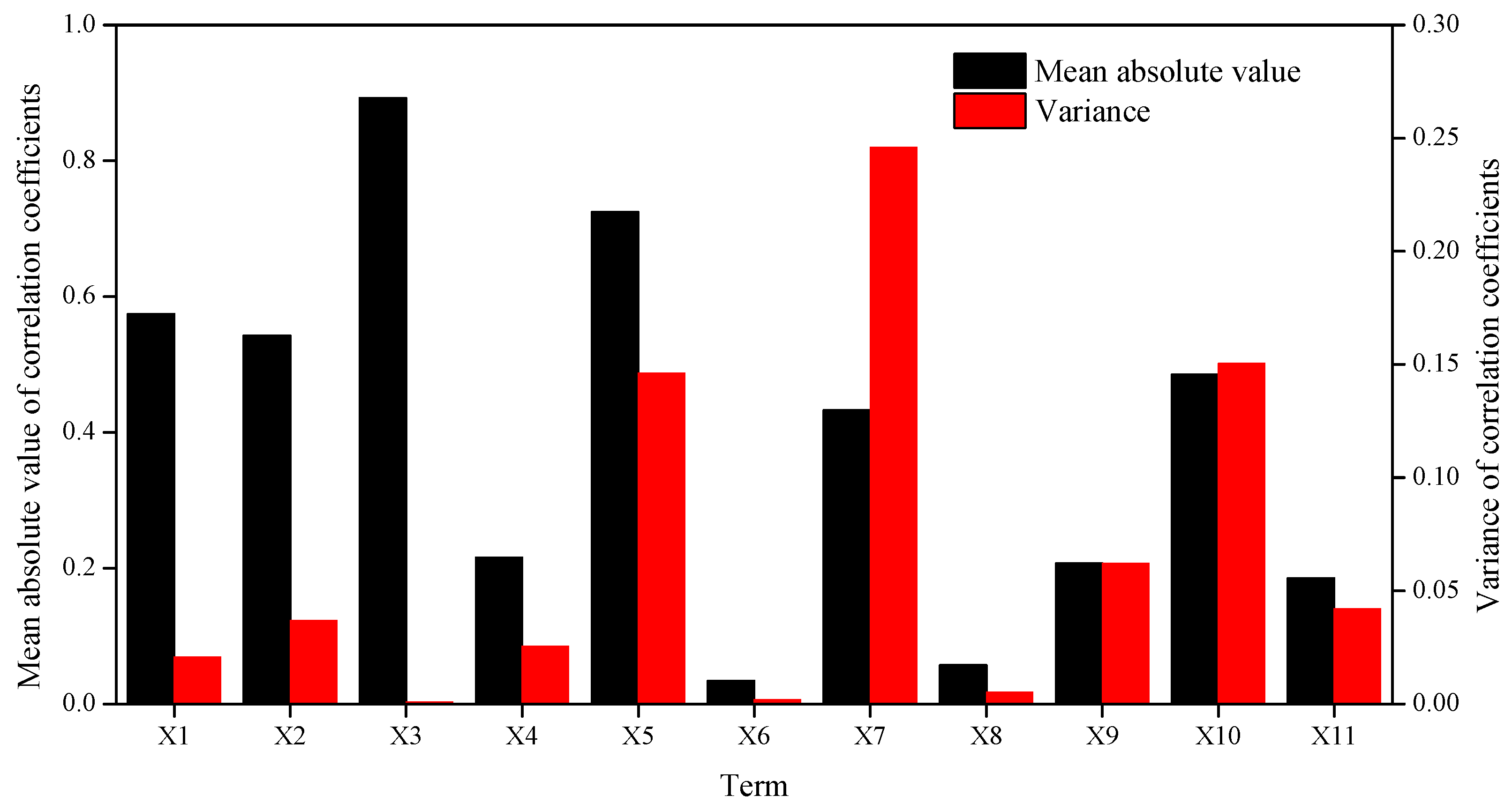
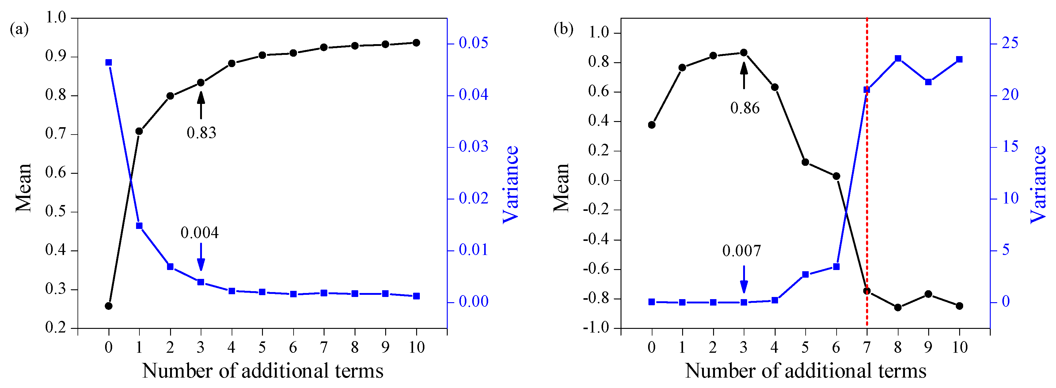
3.1. Single-Factor Analysis

The first term (X1) in Equation (6) is the steady uniform friction term. The 2nd to 5th terms (X2–X5) are additional terms for the first-order time and space partial derivatives of h and u, and the 6th to 11th terms (X6–X11) are additional terms for the second-order time and space partial derivatives of h and u. According to Equations (3)–(5), in a steady uniform friction model, the effect of flow unsteadiness and nonuniformity is neglected making the roughness coefficient being a varying parameter in flood events. This complicates the physical meaning of the roughness coefficient and creates a disadvantage for practical applications. In fact, as a comprehensive description for all the influences of factors related to boundary characteristics and river-bed conditions, the roughness coefficient should be regarded as a fixed constant during a flood event. Additionally, a fixed roughness coefficient for a particular river during a particular period is more practical. Similarly, the parameters in Equation (6) are regarded as constants in a particular simulated river-bed condition—that is, three flood events (i.e., Exps. 1, 2, and 3) with different discharge ranges in the same mode (i.e., Modes 1 to 13) share a common set of parameters. Based on this concept, using the time series of three flood events in each experimental mode, the dependence of unsteady friction on each additional term in Equation (6) was analyzed. The terms in Equation (6) were obtained according to the results of the difference quotient method. The objective friction was calculated using Equation (11). The correlations of each term in Equation (6) with objective friction are shown in

Table 2. Linear correlation coefficients of terms and objective friction at each different experimental mode.

Experimental Mode	Linear Correlation Coefficients of Terms (X1, …, X11) and Objective Friction
	X1	X2	X3	X4	X5	X6	X7	X8	X9	X10	X11
Mode 1	0.70	0.89	−0.86	0.48	−0.24	0.12	0.25	0.26	−0.60	−0.19	−0.59
Mode 2	0.73	0.81	−0.90	0.45	−0.09	0.01	−0.07	0.11	−0.23	0.11	−0.25
Mode 3	0.85	0.84	−0.93	0.51	0.41	−0.02	0.16	0.11	−0.30	−0.09	−0.31
Mode 4	0.72	0.68	−0.89	0.32	0.75	−0.02	−0.88	0.08	−0.15	0.90	−0.26
Mode 5	0.71	0.62	−0.89	0.21	0.79	0.01	0.56	0.08	−0.16	−0.22	−0.23
Mode 6	0.53	0.50	−0.90	0.19	0.83	−0.03	−0.51	0.01	0.17	0.74	0.06
Mode 7	0.43	0.42	−0.85	0.05	0.87	−0.01	0.87	0.03	0.04	0.38	−0.04
Mode 8	0.35	0.40	−0.82	0.05	0.86	−0.02	0.29	0.04	−0.01	0.39	−0.25
Mode 9	0.47	0.39	−0.90	0.12	0.93	−0.04	0.09	0.00	0.18	0.70	−0.07
Mode 10	0.49	0.34	−0.92	0.10	0.92	−0.05	−0.36	0.00	0.23	0.89	0.06
Mode 11	0.56	0.35	−0.94	0.09	0.94	−0.04	0.48	0.00	0.29	0.76	0.16
Mode 12	0.48	0.37	−0.90	0.08	0.92	−0.02	0.90	0.01	0.17	0.66	0.05
Mode 13	0.45	0.45	−0.89	0.15	0.86	−0.05	0.21	−0.01	0.16	0.29	0.10

.

The mean absolute value and variance of correlation coefficients are shown in Figure 5, indicating that the terms with a large correlation are X3, X5, X1, X2, X10, and X7 (sorted by the mean absolute value of correlation). Three additional terms for the first-order partial derivatives of time and space of h and u (X2, X3, and X5) are involved, as well as two additional terms for the second-order partial derivatives of time and space of h and u (X7 and X10). The results indicate that the objective friction is related to the temporal and spatial change rates of mean cross-sectional velocity and flow depth. This shows that it is feasible to improve the unsteady friction simulation accuracy using these additional terms. Besides, the variance of X1, X2, and X3 is small, indicating that their relevant degree with the objective friction is almost the same in different river-bed conditions. The variance of X5, X7, and X10 is relatively large, indicating that although some dependence exists, it is diverse in different river-bed conditions. The correlations of other terms are small.

However, for term X1 with the same structure as the steady uniform friction model and named as the steady uniform friction term, its correlation with objective friction is still too low to support a good simulation. This indicates that the accuracy of term X1 is too low to be used for unsteady friction simulation alone, resulting in some inapplicability (Figure 6). This was analyzed as follows: h, u, and f change during a flood event. According to the model structure of term X1, the calculated friction changes in a flood event depending on the relationship between h and u² (h–u² curve). However, the differences between the phase of calculated and objective frictions are not cause for concern. For example, during the passage of single-peak hydrographs, the peak value of u arises first, followed by the peak value of Q (discharge) and h, as supported by both hydraulic experiments and field data [5]. Thus, the diagram of h and u² is a chronological loop curve with anticlockwise direction (Figure 6a). As a result, the peak and valley values defined by term X1 should occur at the time points A and D separately, indicating that the calculated friction should increase first, reach the peak value, decrease to the valley value, and then increase again. In particular, this also indicates that a decrease should occur during the period between the u and h peaks (Figure 6b). In fact, these conclusions are not supported by the experimental data. Compared with the objective friction, the peak value of term X1 occurs prematurely. Besides, generally only a rising limb and falling limb are present during the objective friction (Figure 6b). This significant phase difference between the steady uniform friction model and objective friction has also been reported by Graf and Song [2].

The phase difference phenomenon described above indicates that the steady uniform or quasi-steady friction model based on kinematic wave approximation is not suitable for unsteady flow [12]. In unsteady flow, the hysteresis between flow depth and mean cross-sectional velocity cannot be neglected [4,5]; this inadvertently disturbs the simulation result when these friction models are applied to unsteady conditions. This is an unexpected model structure error. Further, because a one-to-one relationship exists between h and R, there is no difference between using h and R in friction calculation when considering this unexpected model structure error. Thus, the approximation that R is approximated as h—as adopted in this study—is reasonable. On the other hand, objective unsteady friction is related to the temporal and spatial change rates of mean cross-sectional velocity and flow depth [4,5,7,34]. This shows that it is feasible to improve the 1D friction model structure using terms relating to nonuniform and nonsteady characteristics.

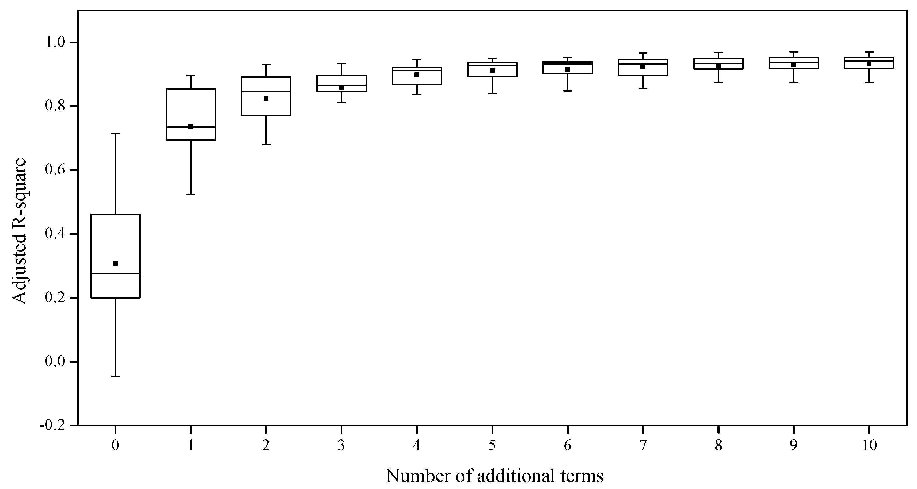
3.2. Multifactorial Analysis

According to the analysis in the previous section, the correlation of each term and objective friction differs. Introduction of irrelevant factors will cause some uncertainty and make the model more unstable; the accuracy is also reduced when correlation factors are omitted. It is essential to determine the optimal number of additional terms and their optimal combination. The entire process can be divided into two steps:

In the first step, the best combination of different numbers of additional terms should be determined. To maintain the applicability in steady uniform flow, term X1 (steady uniform term) was retained. Otherwise, the calculated friction of steady uniform flow using Equation (6) would be zero. X2–X11 are the additional terms that should be evaluated. The number of additional terms increased from 0 to 10; all the different combinations were used for simulation and comparison to determine the best combination. For example, when the number of additional terms was 1, all the possible model structures were X1 + X2, X1 + X3, …, X1 + X11. All of them were used for simulation to determine which one is the best combination when the number of additional term is 1. During the simulation, the terms (X1, X2, …, X11) were obtained using the difference quotient method based on the observed data at three sections. The objective friction was calculated using Equation (11). Then, the parameters for each experimental mode were calibrated using the least-squares method. Degree-of-freedom adjusted coefficient of determination (adjusted R-square) was used to evaluate the model accuracy [35]. The best model structure was determined according to the mean adjusted R-square of 13 different experimental modes. The best model structures for each number of additional terms are listed in

Table 3. Best combinations with different numbers of additional terms.

Number	Best Combination
0	X1
1	X1, X5
2	X1, X2, X3
3	X1, X2, X3, X4
4	X1, X3, X4, X8, X10
5	X1, X3, X4, X7, X8, X10
6	X1, X3, X4, X7, X8, X10, X11
7	X1, X2, X3, X4, X5, X7, X8, X10
8	X1, X2, X3, X4, X5, X7, X8, X10, X11
9	X1, X2, X3, X4, X5, X6, X7, X8, X10, X11
10	X1, X2, X3, X4, X5, X6, X7, X8, X9, X10, X11

. Box plots were used to show their model performances (Figure 7).

In general, the performance of the modified model became better with an increase in the number of additional terms (Figure 7). Without any additional terms, the mean adjusted R-square of the model was low and showed significant instability in different experimental modes [2,9]. After a proper additional term was plugged in, the simulation accuracy and stability of the model improved significantly [3,7]. When the number of additional terms was 3, the accuracy of the modified model was reasonably high. The use of more additional terms did not improve the simulation accuracy.

In the second step, validation tests were performed to determine the exact optimal number of additional terms. In the tests, the experimental data were separated into two groups: for calibration and validation. In each experimental mode, two flood events with discharge ranges of 10–60 and 10–100 m³/h (Exps. 1 and 3) were selected for parameter calibration. For each number of additional terms, the parameters in the best model structure were calibrated using the least-squares method. As a validation, these parameters were used to perform friction simulation in a flood event with a discharge range of 10–80 m³/h (Exp. 2). The validation test was carried out at each experimental mode; thus, up to 13 test results were obtained. In both the calibration and validation, the model performances were evaluated using the adjusted R-square. The mean and variance of adjusted R-square are shown in Figure 8. In the calibration, the performance of different modified models was the same as expected. As the number of additional terms increased, the mean of adjusted R-square increased, and the variance of adjusted R-square decreased (Figure 8a). However, the results of the validation are more complex. When the number of additional terms was 0, 1, 2, and 3, following the improvement of calibration, the validation performance improved. The validation performance was similar to that of calibration. Then, with an increase in the number of additional terms, the validation performance decreased (Figure 8b). This indicates that when the number of additional terms is greater than three (even though more additional terms provide better performance in calibration), there is an overfitting phenomenon that reduces the accuracy of validation phase. This is bad for practical applications. Thus, the optimal number of additional terms is three. The optimal model structure is composed of X1, X2, X3, and X4 (Table 3). The optimal model improved the mean of adjusted R-square in validation from 0.37 to 0.86 and provided a more stable performance (variance of adjusted R-square decreased from 0.044 to 0.007).

Furthermore, according to the continuity equation of the flow [36],

$$\frac{\partial h}{\partial t}+h\frac{\partial u}{\partial x}+u\frac{\partial h}{\partial x}=0$$

(12)

X2, X3, and X5 are related to each other in a linear equality. Thus, in a linear model, one of them can be deduced reversely from the other two. In principle, they cannot be used as additional terms together in linear modified models. This was also verified in the verification test. When the number of additional terms was 7, 8, 9, and 10, the modified models were composed of X2, X3, and X5 together with other terms because too many additional components were required. Their verification accuracies sharply decreased compared with the modified model with six additional terms.

This indicates that the optimal proposed friction model for unsteady flow is theoretically composed of X1 and X4 and two terms among X2, X3, and X5. As a linear model, the proposed modified formula contains three additional terms, yet has considered the effect of four additional terms (i.e., X2, X3, X4, and X5). The modified model can be expressed as follows:

$$f=c_1\frac{u^2}{h}+c_2\frac{u}{h}\frac{\partial h}{\partial t}+c_3\frac{u^2}{h}\frac{\partial h}{\partial x}+c_4\frac{\partial u}{\partial t}$$

(13)

4. Conclusions

Flow resistance is relevant to both the boundary characteristics of a channel and the flow conditions of a stream segment. The partial derivatives of hydraulic parameters are the most relevant physical variables to describe the unsteadiness and nonuniformity of flow condition in a 1D problem. To solve the problem of low accuracy and inapplicability of steady uniform friction models, a linear model with additional terms relating to the first- and second-order time and space partial derivatives of h and u was used to analyze the unsteady flow resistance.

According to the hydraulic experimental data, the unsteady friction is related to the temporal and spatial change rates of mean cross-sectional velocity and flow depth. This shows some feasibility to improve the 1D friction model structure using terms relating to nonuniform and nonsteady characteristics. When these effects were neglected and a steady uniform friction model was used to simulate the unsteady friction, the accuracy was low, resulting in some inapplicability. The analysis results indicate that the hysteresis between flow depth and mean cross-sectional velocity in unsteady flows disturbs the performance of a steady uniform friction model.

To simplify the model structure and improve its practicability, the optimal number and combination of additional terms were evaluated. The results show that the optimal number of additional terms is three, and the optimal model structure is composed of X1, X2, X3, and X4. The optimal model improved the mean of adjusted R-square in validation from 0.37 to 0.86 and showed a more stable performance (variance of adjusted R-square decreased from 0.044 to 0.007).

References

1. Wang, D.W.; Chen, J.G.; Fu, X.D. Review of flow resistance of mountain rivers. J. Hydraul. Eng. 2012, 43, 12–19. [Google Scholar]
2. Graf, W.H.; Song, T. Bed-shear stress in non-uniform and unsteady open-channel flows. J. Hydraul. Res. 1995, 33, 699–704. [Google Scholar] [CrossRef]
3. Ghimire, B.; Deng, Z.-Q. Event flow hydrograph-based method for shear velocity estimation. J. Hydraul. Res. 2011, 49, 272–275. [Google Scholar] [CrossRef]
4. Mrokowska, M.M.; Rowiński, P.M.; Kalinowska, M.B. Evaluation of friction velocity in unsteady flow experiments. J. Hydraul. Res. 2015, 53, 659–669. [Google Scholar] [CrossRef]
5. Mrokowska, M.M.; Rowiński, P.M.; Kalinowska, M.B. A methodological approach of estimating resistance to flow under unsteady flow conditions. Hydrol. Earth Syst. Sci. 2015, 19, 4041–4053. [Google Scholar] [CrossRef]
6. Fread, D.L. Channel Routing. In Hydrological Forecasting; Springer: Cham, Switzerland, 1985. [Google Scholar]
7. Haizhou, T.; Graf, W.H. Friction in unsteady open-channel flow over gravel beds. J. Hydraul. Res. 1993, 31, 99–110. [Google Scholar] [CrossRef]
8. Aleixo, R.; Soares-Frazão, S.; Zech, Y. Velocity-field measurements in a dam-break flow using a PTV Voronoï imaging technique. Exp. Fluids 2011, 50, 1633–1649. [Google Scholar] [CrossRef]
9. Bombar, G. The Hysteresis and Shear Velocity in Unsteady Flows. J. Appl. Fluid Mech. 2016, 9, 839–853. [Google Scholar] [CrossRef]
10. Renaat, S.D.; Verhoeven, R.; Krein, A. Simulation of sediment transport during flood events: Laboratory work and field experiments. Int. Assoc. Sci. Hydrol. Bull. 2001, 46, 599–610. [Google Scholar]
11. Guney, M.S.; Bombar, G.; Aksoy, A.O. Experimental Study of the Coarse Surface Development Effect on the Bimodal Bed-Load Transport under Unsteady Flow Conditions. J. Hydraul. Eng. 2013, 139, 12–21. [Google Scholar] [CrossRef]
12. Henderson, F.M. Flood waves in prismatic channels. J. Hydraul. Div. 1963, 89, 39–67. [Google Scholar]
13. Dey, S.; Lambert, M.F. Reynolds Stress and Bed Shear in Nonuniform Unsteady Open-Channel Flow. J. Hydraul. Eng. 2005, 131, 610–614. [Google Scholar] [CrossRef]
14. Cheng, N.S. Resistance Coefficients for Artificial and Natural Coarse-Bed Channels: Alternative Approach for Large-Scale Roughness. J. Hydraul. Eng. 2015, 141. [Google Scholar] [CrossRef]
15. Roushangar, K.; Mouaze, D.; Shiri, J. Evaluation of genetic programming-based models for simulating friction factor in alluvial channels. J. Hydrol. 2014, 517, 1154–1161. [Google Scholar] [CrossRef]
16. Strupczewski, W.G.; Szymkiewicz, R. Analysis of paradoxes arising from the Chezy formula with constant roughness: II. Flow area-discharge curve. Hydrol. Sci. J. 1996, 41, 659–673. [Google Scholar] [CrossRef]
17. Strupczewski, W.G.; Szymkiewicz, R. Analysis of paradoxes arising from the Chezy formula with constant roughness: I. Depth-discharge curve. Hydrol. Sci. J. 1997, 42, 659–673. [Google Scholar] [CrossRef]
18. Barr, D.I.H.; Ackers, P. Hydraulic design of two-stage channels. Ice Proc. Water Marit. Energy 1992, 106, 99–101. [Google Scholar]
19. Bao, W.M.; Zhang, X.Q.; Qu, S.M. Dynamic correction of roughness in the hydrodynamic model. J. Hydrodyn. Ser. B 2009, 21, 255–263. [Google Scholar] [CrossRef]
20. Hsu, M.H.; Liu, W.C.; Fu, J.C. Dynamic Routing Model with Real-Time Roughness Updating for Flood Forecasting. J. Hydraul. Eng. 2006, 132, 605–619. [Google Scholar] [CrossRef]
21. Bao, H.J.; Zhao, L.N. Hydraulic model with roughness coefficient updating method based on Kalman filter for channel flood forecast. Water Sci. Eng. 2011, 4, 13–23. [Google Scholar]
22. Jin, Z.Q.; Han, L.X.; Zhang, J. The Inverse Problem of Roughness Parameter in Hvdraulic Calculation of Complicated River Net Work. J. Hydrodyn. 1998, 13, 280–285. [Google Scholar]
23. Nikurdase, J. Strömungsgesetze in Rauhen Rohren; VDI Vera: Berlin, Germany, 1933. [Google Scholar]
24. Schlichting, H. Boundary-Layer Theory, 7th ed.; McGraw-Hill: New York, NY, USA, 1979. [Google Scholar]
25. Recking, A. Theoretical development on the effects of changing flow hydraulics on incipient bed load motion. Water Resour. Res. 2009, 45, 1211–1236. [Google Scholar] [CrossRef]
26. Cheng, W.B.; Xie, J.H.; Zhang, R.J. River Dynamics; Wuhan University Press: Wuhan, China, 2007. [Google Scholar]
27. Liu, Z.X.; Li, Z.; Sun, Z.H.; Zheng, Z.P. Calculation of Field Manning’s Roughness Coefficient. Irrig. Drain. 1998, 3, 5–9. [Google Scholar]
28. Nakamura, Y.; Tomonari, Y. The effects of surface roughness on the flow past circular cylinders at high Reynolds numbers. J. Fluid Mech. 1982, 123, 363–378. [Google Scholar] [CrossRef]
29. Einstein, H.A.; Banks, R.B. Fluid resistance of composite roughness. Eos Trans. Am. Geophys. Union 1950, 31, 603–610. [Google Scholar] [CrossRef]
30. Rouse, H. Critical analysis of open-channel resistance. J. Hydraul. Div. 1965, 91, 1–23. [Google Scholar]
31. Salem, A.M. The effects of the sediment bed thick-ness on the incipient motion of particles in a rigid rectangular channel. In Proceedings of the 17th International Water Technology, Istanbul, Turkey, 5–7 November 2013. [Google Scholar]
32. Yan, X.F.; Wai, W.H.O.; Li, C.W. Characteristics of flow structure of free-surface flow in a partly obstructed open channel with vegetation patch. Environ. Fluid Mech. 2016, 16, 1–26. [Google Scholar] [CrossRef]
33. Bombar, G.; Güney, M.Ş.; Tayfur, G.; Elçi, Ş. Calculation of the time-varying mean velocity by different methods and determination of the turbulence intensities. Sci. Res. Essays 2010, 5, 572–581. [Google Scholar]
34. Mrokowska, M.M.; Rowiński, P.M.; Kalinowska, M.B. The Uncertainty of Measurements in River Hydraulics: Evaluation of Friction Velocity Based on an Unrepeatable Experiment. GeoPlanet-Earth Planet. Sci. 2013, 11, 195–206. [Google Scholar]
35. Akossou, A.Y.J.; Palm, R. Impact of data structure on the estimators R-square and adjusted R-square in linear regression. Int. J. Math. Comput. 2013, 20, 84–93. [Google Scholar]
36. Mu, J.B.; Zhang, X.F. Real-time flood forecasting method with 1-D unsteady flow model. J. Hydrodyn. Ser. B 2007, 19, 150–154. [Google Scholar] [CrossRef]
Figure 1. Schematic diagram of experimental setup. (a) plan view; (b) side view.
Water 10 00043 g001
Figure 2. Hydrograph in terms of time variation of discharge at flume entrance in Exp. 2.
Water 10 00043 g002
Figure 3. Representation of relevant points in the discretization method.
Water 10 00043 g003
Figure 4. Evolution of hydraulic parameters at the 1st Section (h1, u1), 2nd Section (h2, u2), 3rd Section (h3, u3), and the evaluated flow depth of nominal point M (h2c, u2c) in Mode 9, Exp. 2. (a) flow depth; (b) mean cross-sectional velocity.
Water 10 00043 g004
Figure 5. Mean absolute value and variance of correlation coefficients.
Water 10 00043 g005
Figure 6. (a) Diagram of h and u2 (hu2 curve) where time points B and C indicate u and h peaks, and time points A and D indicate the peak and valley values calculated by term X1; (b) diagram of h, u, and f during the flood event (Mode 9, Exp. 2), where fo is the objective friction; fc is the calculated friction of term X1 with the same structure as the Chezy formula.
Water 10 00043 g006
Figure 7. Box plots of adjusted R-square with different numbers of additional terms.
Water 10 00043 g007
Figure 8. Mean and variance of adjusted R-square during (a) the calibration period and (b) the validation period.
Water 10 00043 g008