Effects of Guide Vane Placement Angle on Hydraulic Characteristics of Flow Field and Optimal Design of Hydraulic Capsule Pipelines

Abstract

With the rapid growth of agricultural trade volumes, the transportation of agricultural products has received widespread attention from society. Aiming at these problems of low transport efficiency and high transport cost in long-distance transport of agricultural products, an energy-saving and environmental-friendly transport mode of agricultural machinery—hydraulic capsule pipelines (HCPs)—was proposed. HCPs effectively solve issues like traffic congestion, energy crises, and atmospheric pollution. Published literature is mainly limited to the capsule speed and the pressure drop characteristics of the fluid within the pipelines. This research was conducted on the following four aspects of HCPs. Firstly, the structure of the carrier was improved and called a ‘piped carriage’. Secondly, a coupled solution between the structural domain of the piped carriage and the fluid domain within the pipelines was numerically investigated by using the commercial CFD software ANSYS Fluent 12.0 based on the bidirectional fluid–structure interaction methods. Thirdly, the effects of guide vane placement angle on hydraulic characteristics of the internal flow field within the horizontal pipelines transporting the piped carriage were extensively evaluated. Finally, based on least-cost principle, an optimization model of HCPs was established. The results indicated that the simulated results were in good agreement with the experimental results, which further demonstrated that it was feasible to adopt the bidirectional fluid–structure interaction methods for solving the hydraulic characteristics of the internal flow field when the piped carriage was moving along the pipelines. This article will provide an abundant theoretical foundation for the rational design of HCPs and its popularization and application.

1. Introduction

At present, global agricultural product transportation still relied on traditional transportation modes such as railways, highways, waterways, and aviation. Traditional agricultural product transportation modes caused several problems like energy crisis and environmental pollution, which seriously restricted sustainable development between social economy and ecological environment. Aiming at several problems of low transport efficiency and high transport cost in the long-distance transport of agricultural products, a relatively new kind of transport mode of agricultural machinery—hydraulic capsule pipelines (HCPs)—was proposed. The principle of HCPs was to use a kind of fluid to push hollow capsules filled with bulk solid materials through the water-filled pipelines [1]. With its advantages of high transport efficiency, low energy consumption, little pollution of the environment, and continuous stable operation, this technology has gradually developed into the most promising mode of transport in modern agriculture [2].

HCPs were the first proposed in 1960 by the Alberta Research Council in Canada, and later were deeply studied at the Capsule Pipeline Research Center, University of Missouri-Columbia [3]. The first notable investigative studies on HCPs started in the early 1960s when Charles [4] and Ellis [5] established the mathematical model for the flow of a single cylindrical capsule with density equal to that of its carrier fluid (water). Subsequently, Round et al. [6] and Kruyer et al. [7] enhanced the experimental schemes of Charles [4] by taking a single high-density cylindrical capsule as a main research subject, and analyzed relevant relationships between the structural variables and the axial conveyance speed of the single capsule. These studies broadened the density range for the single cylindrical capsule to some extent, but a very limited discussion on the macroscopic speed of the single cylindrical capsule was presented. In the late 1970s hydraulic pipeline transport on more than one capsule was studied by Latto et al. [8] and Tomita et al. [9]. They established the discontinuous capsules transport models and solved the instantaneous axial speed of the capsules by using the method of characteristics, but considered the capsules as point masses and offered the limited discussion on the hydraulic characteristics of the internal flow field within the pipelines.

In the mid-1980s, many experts analyzed the dynamic characteristics of single-capsule transport from the perspective of annular slit flow. The mathematical models of the turbulent flow in an annular slit areas were first established by Kroonenberg [10], who analyzed the hydraulic characteristics of the annular slit flow including velocity distributions, pressure distributions, and boundary shear forces. Polderman et al. [11] explored the hydraulic characteristics for the lubricating fluid in the annular slit areas when the single cylindrical capsule was moving within the pipelines, and compared three-layer gradient diffusion models with the experimental results. Chow [12] and Sud et al. [13] extended Kroonenberg’s [10] studies. They analyzed the fully developed turbulent flow models within the annular slit areas under the moving boundary by adopting basic relationships of the turbulent flow. In the early 1990s, based on the three motion stages (suspension, oscillation, and stable migration), Fujiwara et al. [14] adopted the method of model testing to analyze the flow characteristics of both laminar and turbulent capsule flows in the annular slit areas under the conditions of both the concentric and eccentric conveying pipes. Cheng et al. [15], Lenau et al. [16], and Huang et al. [17] assumed that the single cylindrical capsule was both an elastic capsule model and a rigid capsule model. By using these two models, these researchers predicted the critical velocity required to cause tilting of a single cylindrical capsule when movement by a liquid flowing within the horizontal pipelines was obstructed by the presence of an obstacle or protrusion on the pipe wall. Agarwal [18] and Vlasak [19] used dimensional analysis to analyze the effects of different physical factors on the capsule speeds. Yanaida et al. [20] and Azouz et al. [21] supplemented Polderman et al.’s [11] research findings. They highlighted the turbulence vortex viscosity models to predict the hydraulic characteristics of the annular slit flow formed by a Newtonian fluid, non-Newtonian fluid, and drag-reducing fluid under a moving boundary, which further perfected the correlative theories of the annular slit flow.

In the early 21st century, Sun et al. [22] studied the relationship between the transport loadings and the incipient velocities under the critical start-up condition of the cylindrical capsules within the pipelines. An extension of Sun et al.’s [22] work was made by Wang et al. [23] and Li et al. [24] who divided the overall transport processes into different stages and revealed the power sources of every stage by analyzing the hydrodynamic mechanisms for the single cylindrical capsule. Zhang et al. [25] conducted a wide range of experimental investigations to analyze the pressure drop characteristics of the annular slit flow when the single cylindrical capsule transported within the pipelines under different discharge and loading conditions. Wang et al. [26] added Zhang et al.’s [25] research schemes and proposed the concepts of the optimal transport Reynolds number for the cylindrical capsule transport from the perspective of energy loss ratio inside the round pipelines. However, their studies lacked detailed analysis on the flow velocity distributions and the pressure distributions of the internal flow field inside the pipelines.

As computer technologies mature, numerical simulation was being widely applied to solve a variety of complex hydraulics problems. The transport of heavy-density cylindrical capsules within the vertical and horizontal pipelines was studied numerically by Vlasak et al. [27]. Subsequently, Ulusarslan [28] discussed the pressure drop characteristics caused by a train of varying-density spherical capsules within the pipelines. Khalil et al. [29] used three different turbulent models to develop a numerical solution for the fundamental equations governing turbulent flow around a single, concentric, long capsule in a pipe, which revealed the preliminary velocity distributions and pressure distributions of the internal flow field around the cylindrical capsules. Asim et al. [30,31] conducted detailed numerical analysis on the hydraulic characteristics of fluids transporting rectangular and cylindrical capsules and proposed a semi-empirical model for predicting the pressure drop characteristics in HCPs. Further studies carried out by Li et al. [32], who analyzed the hydraulic characteristics of transporting the cylindrical capsules by using commercial CFD software Flow-3D 9.3 within the pipelines. These studies focused only on the unidirectional fluid–structure interaction such that the capsule movement was assumed to be uniform motion with a constant speed within the pipelines. Feng et al. [33] conducted a series of analytical studies on a bidirectional fluid–structure interaction between an elliptic capsule and laminar fluid. However, these studies only involved the bidirectional fluid–structure interaction between the elliptic capsule and the Poiseuille flow in a two-dimensional channel, failing to reflect the bidirectional fluid–structure interaction between the capsules and a three-dimensional turbulent fluid within the round pipelines.

In order to further improve the transport efficiency of the cylindrical capsules within the pressurized pipelines, an improved cylindrical capsule was proposed and defined as a ‘piped carriage’. In recent years, the numerical simulation of the bidirectional fluid–structure interaction has become an important tool of fluid machinery analysis, which considered the interaction between the fluid domain and the structural domain so that the computational results were closer to real physical phenomena. At present, the numerical simulation of the bidirectional fluid–structure interaction was mainly applied to the research findings in the rotating machineries such as the centrifugal pumps [34], the fans [35] and the turbines [36], but a very limited discussed on the piped carriage in HCPs has been presented. In this study, the bidirectional fluid–structure interaction between the structural domain of the piped carriage and the fluid domain within the pipelines was numerically investigated by using the commercial CFD software ANSYS-Fluent 12.0, and the effects of guide vane placement angle on the hydraulic characteristics of transporting the piped carriage within the horizontal pipelines were studied by identifying average speeds, velocity distributions, pressure distributions, vorticity magnitude distributions, pressure drop characteristics, mechanical efficiencies, as well as force statistics during the movement of the single piped carriage. At the same time, based on least cost principle, an optimization model of HCPs transporting the piped carriage was established. This article will help to accurately master the change laws of the velocity distributions and the pressure distributions in a HCPs, and provide a solid theoretical foundation for the rational determination of the technical elements in a HCPs and an accurate evaluation of its transport effects.

This remainder of this article is organized as follows. Chapter 2 and 3 express the relevant theories, and materials and methods of the model testing for the piped carriage transport respectively. In Chapter 4, the numerical methods of the bidirectional fluid–structure interaction are analyzed in detail. Chapter 5 expresses the verification of the simulated results in order to improve its reliability. Chapter 6 discusses the simulated results of the hydraulic characteristics within the internal flow field transporting the piped carriage having different guide vane placement angles. An optimization model of HCPs transporting the piped carriage is established based on least cost principle in Chapter 7. Chapter 8 gives summary and expectation of this article.

2. Theoretical Analysis

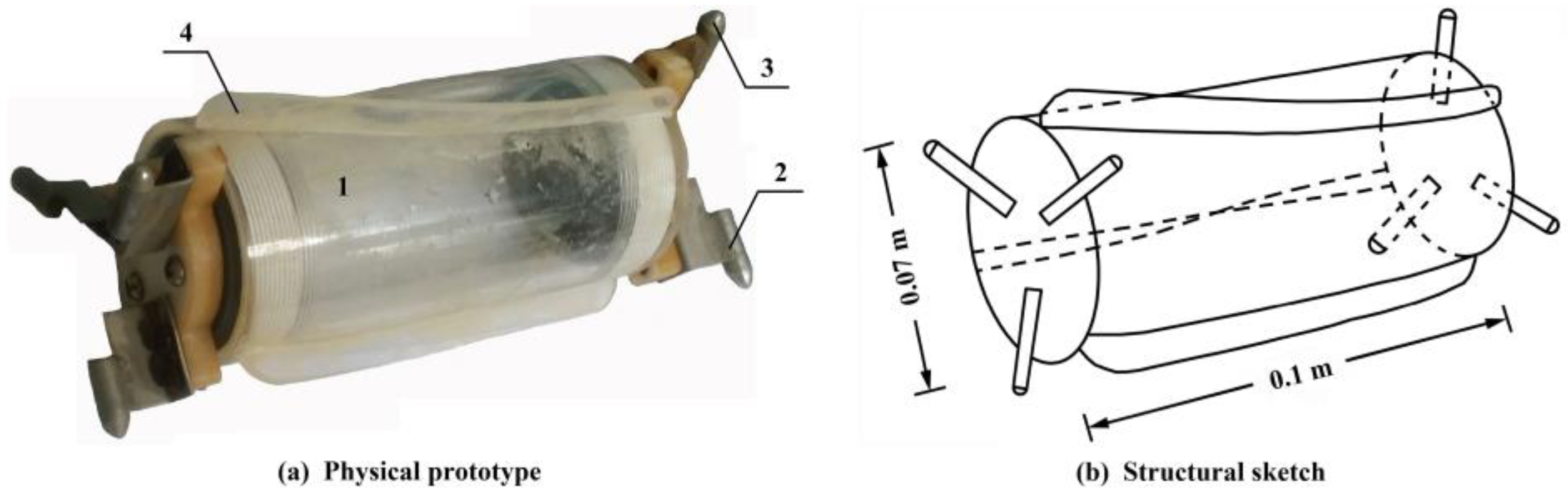
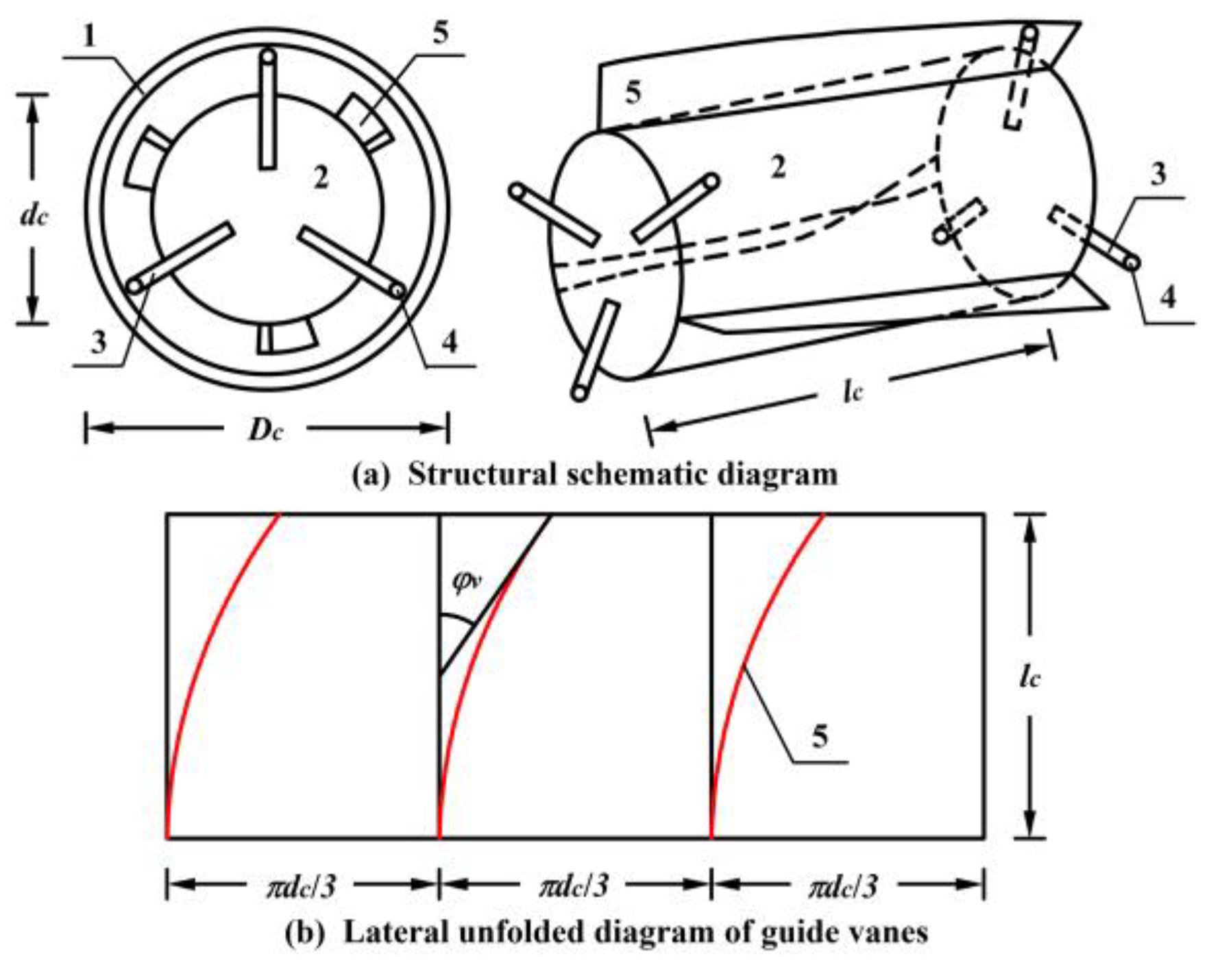
2.1. Design of the Piped Carriage

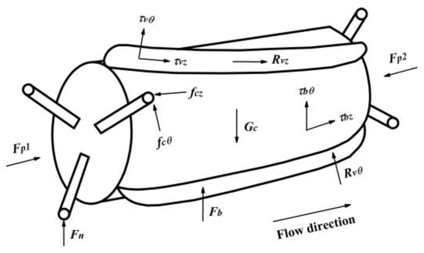
In recent years, the researchers have proposed a variety of the transport capsules. According to the corresponding different structural types, the capsules were divided into five categories such as a spherical capsule [28], a cylindrical capsule [10,14,30], a hexahedral capsule [31], a cylindrical capsule with wheels [37], and a cylindrical capsule with supports [22]. When transporting the materials in a 180° pipe bend, the cylindrical capsule and the hexahedral capsule collided with the inner wall of its conveying pipes, which reduced the service life of the conveying pipes. The cylindrical capsule with wheels and the cylindrical capsule with supports maintained the concentric state with the conveying pipes, which prevented the capsules from repeated vibrations caused by the velocity variation that occurred suddenly throughout the pressure pipelines. At the same time, the wheels and the universal balls at the end of the support bodies caused the rolling frictional resistance with the inner wall of the conveying pipes during the movement of the capsules, which reduced the degree of wear for the inner wall of the conveying pipes. The spherical capsules had better kinetic stability during transport. However, because of the limitations of the pipe diameter, the internal space of the capsule was so small that a large amount of bulk solid materials cannot be sufficiently transported. The ‘piped carriage’ proposed in this article improved the above-mentioned capsules by installing the guide-vane structure on the outer wall of the cylindrical capsule. On the one hand, the guide vanes caused the piped carriage to rotate itself and improved the stability of the material transport. On the other hand, the guide vanes increased the areas that were affected by the pipe fluid on the piped carriage and improved its transport efficiency. Compared with more capsules in the previous published literature, the piped carriage had the advantages of obvious structural innovation. The piped carriage was composed by four parts: a barrel, support bodies, universal balls, and guide vanes. The entity structure of the piped carriage was shown in Figure 1.

The barrel was a cylinder that machined from Plexiglas with a thickness of 5 mm, and its two ends were connected to screw caps by threads [25]. In this article, the length and the diameter of the barrel were defined as the length and the diameter of the piped carriage respectively, which were expressed with symbols of l_c and d_c respectively. The support body of the piped carriage was composed of a thin cylinder and a sheet-metal plate, and radially arranged on the front and rear ends of the cylindrical barrel structure at 120-degree angles from each other [24]. The support bodies always maintained a concentric position of the piped carriage within the transmission pipelines, which avoided the collision between the piped carriage and the conveying pipes. In addition, the universal balls were mounted at the end of each support body in order to reduce the frictional resistance between the piped carriage wall and the pipe internal wall, thus contributing to energy efficiency. The guide vanes were made of thick Plexiglas with a thickness of 3 mm by using the wooden molds and interlaced with the support bodies at intervals of 60-degree angles on the outer wall of the barrel. The guide vane was not a plane but a twisted surface. The long side of the guide vane was connected to the outer wall of the barrel, and its short side was perpendicular to the tangent to the outer wall of the barrel at the fixed point. The projection length of the long side along the pipe axis and the short side were defined as the length and the height of the guide vanes, respectively, which were expressed with symbols of l_v and h_v, respectively. In the lateral unfolded diagram of the barrel, any point on the sideline of its rear end was regarded as a reference point. Every additional 5 mm in line segment along the pipe axis increased the same deflection angle to the outer side. The smooth curve that was used to connecting the intersections of the line segments was the placement path of the guide vanes on the outer wall of the barrel. The maximum deflection angle of the accumulated line segment was the placement angle of the guide vanes, which was expressed with a symbol of φ_v. The guide vanes were arranged anticlockwise from the rear end of the barrel to its front end. In order to reduce the transport resistance of transporting the piped carriage, both ends of the guide vanes were machined into streamlined structure. The guide vanes caused the translation and rotation with the aid of water thrust force, thereby realizing the stable migration of the piped carriage. Steel ball bearings having a diameter of 8 mm were served inside the single piped carriage and defined as a transport loading of the piped carriage. The space between the steel ball bearings was filled with rubber marine sand which had gelling properties. The structural diagram of the piped carriage was shown in Figure 2.

2.2. Force Analysis

The piped carriage was taken as the research object. When the piped carriage transported within the horizontal pipelines, the forces acting on it mainly included:

(1)

The gravity of the piped carriage G_c was related to the basic materials of the piped carriage.

(2)

The pressure gradient force acting on the front and rear ends of the piped carriage F_p, which can be expressed as

$$F_p=F_{p1}-F_{p2}$$

(1)

where F_p1 and F_p2 were the fluid pressures acting on the front and rear ends of the piped carriage, respectively.

(3)

The support force of the pipe wall against the piped carriage F_n. Six support forces acting on the contact points between the universal balls of the piped carriage and the inner wall of the pipes in different directions, and the directions of these support forces pointed towards the center of the conveying pipes from its interior wall.

(4)

The buoyancy of the piped carriage F_b was related to the internal volume of the barrel.

(5)

The rolling frictional resistance f_c was decomposed into an axial force f_cz and a circumferential force f_cθ. These two forces can be expressed respectively as

$$f_{cz}={\mu }_z{F}_n,f_{c\theta }={\mu }_{\theta }{F}_n$$

(2)

where μ_z was the axial rolling frictional resistance coefficient, μ_θ was the circumferential rolling frictional resistance coefficient.

(6)

The shear stress of the annular slit flow acting on the sidewall of the guide vanes τ_v was decomposed into an axial force τ_vz and a circumferential force τ_vθ. These two forces can be expressed respectively as

$${\tau }_{vz}=\frac{{\lambda }_v\rho {\left(V_{az}-U_{vz}\right)}^2}{8},{\tau }_{v\theta }=\frac{{\lambda }_v\rho {\left(V_{a\theta }-U_{v\theta }\right)}^2}{8}$$

(3)

where V_az and V_aθ were the average axial speed and the average circumferential speed of the piped carriage respectively; U_vz and U_vθ were the average axial velocity and the average circumferential velocity of the annular slit flow in the near-wall areas of the guide vanes respectively; λ_v was the flow resistance coefficient in the near-wall areas of the guide vanes; ρ was the fluid density. In this article, the average circumferential speed and average angular speed of the piped carriage represented the circumferential rotating speed of the piped carriage, but the emphases expressed by these two physical parameters were different. The average axial velocity was analyzed by using the arc length, while the average angular velocity was analyzed by using the rotation angle.

(7)

The shear stress of the annular slit flow acting on the sidewall of the barrel τ_b was decomposed into an axial force τ_bz and a circumferential force τ_bθ. These two forces can be expressed respectively as

$${\tau }_{bz}=\frac{{\lambda }_b\rho {\left(V_{az}-U_{sz}\right)}^2}{8},{\tau }_{b\theta }=\frac{{\lambda }_b\rho {\left(V_{a\theta }-U_{s\theta }\right)}^2}{8}$$

(4)

where U_sz and U_sθ were the average axial velocity and the average circumferential velocity of the annular slit flow respectively; λ_b was the flow resistance coefficient in the near-wall areas of the barrel.

(8)

The fluid thrust acting on the guide vanes R_v was decomposed into an axial force R_vz and a circumferential force R_vθ. These two forces can be expressed respectively as

$$\begin{gathered} R_{vz}=\frac{\psi C_{z}sin{\phi }_v{l}_v{h}_v{\left(U_{av}-V_{az}\right)}^2}{2},R_{v\theta }=\frac{\psi C_{\theta }sin{\phi }_v{l}_v{h}_v{\left(U_{av}-V_{az}\right)}^2}{2} \\ {C}_z=C_{\theta }=0.026R{e}^{-\frac{1}{7}} \end{gathered}$$

(5)

where C_z and C_θ were the axial thrust coefficient and the circumferential thrust coefficient of the guide vanes respectively; ψ was the projected area coefficient of the guide vanes in the direction vertical to the pipe fluid; U_av was the average axial velocity of the pipe fluid.

(9)

The lift acting on the piped carriage F_l was related to the hydrodynamic pressure and the average axial velocity of the pipe fluid.

The force analysis on the piped carriage was shown in Figure 3.

2.3. Motion Model

According to the force characteristics of the piped carriage, the motion models of transporting the piped carriage within the horizontal pipelines were established.

According to the law of mass conservation, the total fluid mass m_a flowing into the pipe was equal to the sum of both the fluid mass m_c flowing into the pipe due to the displacement of the piped carriage and the fluid mass m_s flowing into the pipe through the annular slit space during the ∆t period. When the piped carriage moved at a constant speed, the continuity equation of the fluid inside the pipelines can be expressed as

$$m_a=m_c+m_s$$

(6)

During the ∆t period, the total fluid mass flowing into the pipe can be expressed as

$$m_a=\frac{U_{av}{D}_c^2}{4}\rho \Delta t$$

(7)

During the ∆t period, the fluid mass flowing into the pipe due to the displacement of the piped carriage can be expressed as

$$m_c=\frac{V_{az}{d}_c^2}{4}\rho \Delta t$$

(8)

During the ∆t period, the fluid mass flowing into the pipe through the annular slit space can be expressed as

$$m_s=\frac{U_{sz}\left(D_c^2-d_c^2\right)}{4}\rho \Delta t$$

(9)

Substituting Equations (7)–(9) into Equation (6) to obtain

$$\frac{U_{av}{D}_c^2}{4}\rho \Delta t=\frac{V_{az}{d}_c^2}{4}\rho \Delta t+\frac{U_{sz}\left(D_c^2-d_c^2\right)}{4}\rho \Delta t$$

(10)

where D_c and d_c were the diameters of the conveying pipes and the piped carriage, respectively.

Assuming that the diameter ratio of the piped carriage can be expressed as

$$b=\frac{d_c}{D_c}$$

(11)

Substituting Equation (11) into Equation (10) to obtain the average axial velocity of the annular slit flow. This average axial velocity can be expressed as

$$U_{sz}=\frac{U_{av}-b^2{V}_{az}}{1-b^2}$$

(12)

When the piped carriage moved steadily along the pipe axis within the pipelines, the forces acting on the piped carriage and the annular slit flow in the part where the piped carriage was respectively should reach equilibrium states.

When the average axial velocity of the annular slit flow was greater than the average axial speed of the piped carriage, the direction of the shear stress acting on the piped carriage was oriented in the same direction as the pipe fluid, and then the shear stress was the power of the piped carriage, otherwise the shear stress was the resistance of the piped carriage.

If the shear stress acting on the piped carriage was power, then the forces acting on the piped carriage along the pipe axis included the pressure gradient force acting on the front and rear ends of the piped carriage F_p, the axial force of the shear forces for the annular slit flow acting on the sidewall of the barrel T_bz, the axial force of the shear forces for the annular slit flow acting on the sidewall of the guide vanes T_vz, the axial force of the fluid thrust acting on the guide vanes R_vz and the axial force of the rolling frictional resistance f_cz.

According to Equation (1), the pressure gradient force acting on the front and rear ends of the piped carriage can be expressed as

$$F_p=\frac{\pi d_c^2\Delta p_c}{4}$$

(13)

where ∆p_c was the fluid pressure difference between the front and rear ends of the piped carriage.

According to Equation (4), the axial force of the shear forces for the annular slit flow acting on the sidewall of the barrel can be expressed as

$$T_{bz}={\tau }_{bz}{d}_c{l}_c\pi =\frac{{\lambda }_b\rho {\left(V_{az}-U_{sz}\right)}^2{d}_c{l}_c\pi }{8}$$

(14)

According to Equation (3), the axial force of the shear forces for the annular slit flow acting on the sidewall of the guide vanes can be expressed as

$$T_{vz}={\tau }_{vz}{h}_v{l}_v=\frac{{\lambda }_v\rho {\left(V_{az}-U_{vz}\right)}^2{h}_v{l}_v}{8}$$

(15)

According to the Equation (2), the axial force of the rolling frictional resistance f_cz was obtained, and according to the Equation (5), the axial force of the fluid thrust acting on the guide vanes R_vz was calculated.

The pressure gradient force acting on the front and rear ends of the piped carriage F_p, the axial force of the shear forces for the annular slit flow acting on the sidewall of the barrel T_bz, the axial force of the shear forces for the annular slit flow acting on the sidewall of the guide vanes T_vz and the axial force of the fluid thrust acting on the guide vanes R_vz were powers, while the axial force of the rolling frictional resistance f_cz was resistance. The powers and resistance were always equal and opposite.

Therefore, for the piped carriage, the force balanced equations in the direction of the pipe axis can be expressed as

$$F_p+T_{bz}+R_{vz}+T_{vz}=f_{cz}$$

(16)

Substituting Equations (2), (5) and (13)–(15) into Equation (16) to obtain

$$\begin{array}{l}\frac{\pi d_c^2\Delta p_c}{4}+\frac{{\lambda }_b\rho {\left(V_{az}-U_{sz}\right)}^2{d}_c{l}_c\pi }{8}+0.5\psi C_{z}sin{\phi }_v{l}_v{h}_v{\left(U_{av}-V_{az}\right)}^2\\ +\frac{{\lambda }_v\rho {\left(V_{az}-U_{vz}\right)}^2{h}_v{l}_v}{8}=f_{cz}\end{array}$$

(17)

The fluid pressure difference between the front and rear ends of the piped carriage was deduced from Equation (17), which can be expressed as

$$\begin{array}{l}\Delta p_c=\frac{4{\mu }_z{F}_n}{\pi d_c^2}-\frac{{\lambda }_b\rho {\left(V_{az}-U_{sz}\right)}^2{d}_c{l}_c\pi }{2\pi d_c^2}\\ -\frac{2C_z\psi sin{\phi }_v{l}_v{h}_v{\left(U_{av}-V_{az}\right)}^2}{\pi d_c^2}-\frac{{\lambda }_v\rho {\left(V_{az}-U_{vz}\right)}^2{h}_v{l}_v}{2\pi d_c^2}\end{array}$$

(18)

The annular slit flow in the part where the piped carriage was along the pipe axis included the pressure gradient force acting on the front and rear cross-sections of the annular slit flow N_p, and the axial force of the shear forces for the sidewall of the barrel acting on the annular slit flow S_bz and the axial force of the shear forces for the sidewall of the guide vanes acting on the annular slit flow S_vz, the shear forces of the pipe wall acting on the annular slit flow S_p, and the axial force of the fluid thrust of the guide vane acting on the annular slit flow W_vz.

The pressure gradient force acting on the front and rear cross-sections of the annular slit flow in the part where the piped carriage was can be expressed as

$$N_p=\frac{\pi \left(D_c^2-d_c^2\right)\Delta p_s}{4}$$

(19)

where ∆p_s was the fluid pressure difference between the front and rear cross-sections of the annular slit flow in the part where the piped carriage was.

According to Equation (4), the axial force of the shear forces for the sidewall of the barrel acting on the annular slit flow can be expressed as

$$S_{bz}={\tau }_{bz}{d}_c{l}_c\pi =\frac{{\lambda }_b\rho {\left(V_{az}-U_{sz}\right)}^2{d}_c{l}_c\pi }{8}$$

(20)

According to Equation (3), the axial force of the shear forces for the sidewall of the guide vanes acting on the annular slit flow can be expressed as

$$S_{vz}={\tau }_{vz}{h}_v{l}_v=\frac{{\lambda }_v\rho {\left(V_{az}-U_{vz}\right)}^2{h}_v{l}_v}{8}$$

(21)

The shear forces of the pipe wall acting on the annular slit flow can be expressed as

$$S_p={\tau }_p\pi D_c{l}_c$$

(22)

The shear stress acting on the interior wall of the conveying pipes can be expressed as

$${\tau }_p=\frac{{\lambda }_p\rho U_{sz}^2}{8}$$

(23)

where λ_p was the flow resistance coefficient in the near-wall areas of the pipe wall.

Substituting Equation (23) into Equation (22) to obtain

$$S_p=\frac{{\lambda }_p\rho U_{sz}^2\pi D_c{l}_c}{8}$$

(24)

According to Equation (5), the axial force of the fluid thrust of the guide vane acting on the annular slit flow can be expressed as

$$W_{vz}=\frac{\psi C_{z}sin{\phi }_v{l}_v{h}_v{\left(U_{av}-V_{az}\right)}^2}{2}$$

(25)

The pressure gradient force acting on the front and rear cross-sections of the annular slit flow was power, while the axial force of the shear forces for the sidewall of the barrel acting on the annular slit flow S_bz and the axial force of the shear forces for the sidewall of the guide vanes acting on the annular slit flow S_vz, the shear forces of the pipe wall acting on the annular slit flow S_p, and the axial force of the fluid thrust of the guide vane acting on the annular slit flow W_vz were resistances. The power and resistances were always equal and opposite.

Therefore, for the annular slit flow in the part where the piped carriage was, the force balanced equations in the direction of the pipe axis can be expressed as

$$N_p=S_p+S_{bz}+W_{vz}+S_{vz}$$

(26)

Substituting Equations (19)–(21), (24) and (25) into Equation (26) to obtain

$$\begin{array}{l}\frac{\pi \left(D_c^2-d_c^2\right)\Delta p_s}{4}=\frac{{\lambda }_p\rho U_{sz}^2\pi D_c{l}_c}{8}+\frac{{\lambda }_b\rho {\left(V_{az}-U_{sz}\right)}^2{d}_c{l}_c\pi }{8}\\ +\frac{\psi C_{z}sin{\phi }_v{l}_v{h}_v{\left(U_{av}-V_{az}\right)}^2}{2}+\frac{{\lambda }_v\rho {\left(V_{az}-U_{vz}\right)}^2{h}_v{l}_v}{8}\end{array}$$

(27)

The differential pressure between the front and rear cross-sections of the annular slit annular slit flow was deduced from Equation (27), which can be expressed as

$$\begin{array}{l}\Delta p_s=\frac{{\lambda }_p\rho U_{sz}^2{D}_c{l}_c}{2\left(D_c^2-d_c^2\right)}+\frac{{\lambda }_b\rho {\left(V_{az}-U_{sz}\right)}^2{d}_c{l}_c}{2\left(D_c^2-d_c^2\right)}\\ +\frac{2C_z\psi sin{\phi }_v{l}_v{h}_v{\left(U_{av}-V_{az}\right)}^2}{\pi \left(D_c^2-d_c^2\right)}+\frac{{\lambda }_v\rho {\left(V_{az}-U_{vz}\right)}^2{h}_v{l}_v}{2\pi \left(D_c^2-d_c^2\right)}\end{array}$$

(28)

Since the fluid pressure difference between the front and rear ends of the piped carriage ∆p_c was equal to the fluid pressure difference between the front and rear cross-sections of the annular slit flow in the part where the piped carriage was ∆p_s, it was possible to obtain

$$\begin{array}{l}\frac{4{\mu }_z{F}_n}{\pi d_c^2}-\frac{{\lambda }_b\rho {\left(V_{az}-U_{sz}\right)}^2{d}_c{l}_c\pi }{2\pi d_c^2}-\frac{2C_z\psi sin{\phi }_v{l}_v{h}_v{\left(U_{av}-V_{az}\right)}^2}{\pi d_c^2}\\ -\frac{{\lambda }_v\rho {\left(V_{az}-U_{vz}\right)}^2{h}_v{l}_v}{2\pi d_c^2}=\frac{{\lambda }_p\rho U_{sz}^2{D}_c{l}_c}{2\left(D_c^2-d_c^2\right)}+\frac{{\lambda }_b\rho {\left(V_{az}-U_{sz}\right)}^2{d}_c{l}_c}{2\left(D_c^2-d_c^2\right)}\\ +\frac{2C_z\psi sin{\phi }_v{l}_v{h}_v{\left(U_{av}-V_{az}\right)}^2}{\pi \left(D_c^2-d_c^2\right)}+\frac{{\lambda }_v\rho {\left(V_{az}-U_{vz}\right)}^2{h}_v{l}_v}{2\pi \left(D_c^2-d_c^2\right)}\end{array}$$

(29)

Let $\zeta =\frac{U_{sz}}{U_{vz}}$.

The motion models of transporting the piped carriage were deduced from Equation (29), which can be expressed as

$$A_1{V}_{az}^2+B_1{U}_{av}{V}_{az}+C_1{U}_{av}^2-\frac{4{\tau }_{bz}{d}_c{l}_c\pi +4{\mu }_z{F}_n-4{\tau }_{vz}{h}_v{l}_v}{\pi b^2{D}_c^2}=0$$

(30)

where

$$\begin{gathered} A_1=\frac{b^4{\lambda }_p\rho D_c{l}_c\pi +{\lambda }_b\rho d_c{l}_c\pi +{\left(1-b^2+\zeta b^2\right)}^2{\lambda }_v\rho h_v{l}_v}{2\pi D_c^2{\left(1-b^2\right)}^3}+\frac{2C_z\psi sin{\phi }_v{l}_v{h}_v}{\pi D_c^2{b}^2}+\frac{2C_z\psi sin{\phi }_v{l}_v{h}_v}{\pi D_c^2\left(1-b^2\right)} \\ {B}_1=\frac{{\lambda }_b\rho d_c{l}_c-2b^2{\lambda }_p\rho D_c{l}_c-2\zeta \left(1-b^2+\zeta b^2\right){\lambda }_v\rho h_v{l}_v}{2D_c^2{\left(1-b^2\right)}^3}-\frac{4C_z\psi sin{\phi }_v{l}_v{h}_v}{\pi D_c^2{b}^2}+\frac{2C_z\psi sin{\phi }_v{l}_v{h}_v}{\pi D_c^2\left(1-b^2\right)} \\ {C}_1=\frac{{\lambda }_p\rho D_c{l}_c\pi +{\lambda }_b\rho d_c{l}_c\pi +{\zeta }^2{\lambda }_v\rho h_v{l}_v}{2\pi D_c^2{\left(1-b^2\right)}^3}+\frac{2C_z\psi sin{\phi }_v{l}_v{h}_v}{\pi D_c^2\left(1-b^2\right)}+\frac{2C_z\psi sin{\phi }_v{l}_v{h}_v}{\pi b^2{D}_c^2} \end{gathered}$$

According to Equation (30), the average axial speed of the piped carriage can be expressed as

$$V_{az}=\sqrt{\frac{B_1^2{U}_{av}^2}{4A_1^2}-\frac{C_1{U}_{av}^2}{A_1}+\frac{4{\tau }_{bz}{d}_c{l}_c\pi +4{\mu }_z{F}_n-4{\tau }_{vz}{h}_v{l}_v}{A_1\pi b^2{D}_c^2}}$$

(31)

If the shear stress acting on the piped carriage was resistance, then based on the forces acting on the piped carriage along the pipe axis, the pressure gradient force acting on the front and rear ends of the piped carriage F_p, and the axial force of the fluid thrust acting on the guide vanes R_vz were powers, while the axial force of the shear forces for the annular slit flow acting on the sidewall of the barrel T_bz, the axial force of the shear forces for the annular slit flow acting on the sidewall of the guide vanes T_vz, the axial force of the rolling frictional resistance f_cz were resistances. The powers and resistances were always equal and opposite.

Therefore, for the piped carriage, the force balanced equations in the direction of the pipe axis can be expressed as

$$F_p-T_{bz}+R_{vz}-T_{vz}=f_{cz}$$

(32)

Substituting Equations (2), (5), and (13)–(15) into Equation (32) to obtain

$$\begin{array}{l}\frac{\pi d_c^2\Delta p_c}{4}-\frac{{\lambda }_b\rho {\left(V_{az}-U_{sz}\right)}^2{d}_c{l}_c\pi }{8}+\frac{\psi C_{z}sin{\phi }_v{l}_v{h}_v{\left(U_{av}-V_{az}\right)}^2}{2}\\ -\frac{{\lambda }_v\rho {\left(V_{az}-U_{vz}\right)}^2{h}_v{l}_v}{8}=f_{cz}\end{array}$$

(33)

The fluid pressure difference between the front and rear ends of the piped carriage was deduced from Equation (33), which can be expressed as

$$\begin{array}{l}\Delta p_c=\frac{4{\mu }_z{F}_n}{\pi d_c^2}+\frac{{\lambda }_b\rho {\left(V_{az}-U_{sz}\right)}^2{d}_c{l}_c\pi }{2\pi d_c^2}\\ -\frac{2C_z\psi sin{\phi }_v{l}_v{h}_v{\left(U_{av}-V_{az}\right)}^2}{\pi d_c^2}+\frac{{\lambda }_v\rho {\left(V_{az}-U_{vz}\right)}^2{h}_v{l}_v}{2\pi d_c^2}\end{array}$$

(34)

Based on the annular slit flow in the part where the piped carriage was along the pipe axis, the pressure gradient force acting on the front and rear cross-sections of the annular slit flow N_p, the axial force of the shear forces for the sidewall of the barrel acting on the annular slit flow S_bz and the axial force of the shear forces for the sidewall of the guide vanes acting on the annular slit flow S_vz were powers, while the shear forces of the pipe wall acting on the annular slit flow S_p, and the axial force of the fluid thrust of the guide vane acting on the annular slit flow W_vz were resistances. The power and resistances were always equal and opposite.

Therefore, for the annular slit flow in the part where the piped carriage was, the force balanced equations in the direction of the pipe axis can be expressed as

$$N_p=S_p-S_{bz}+W_{vz}-S_{vz}$$

(35)

Substituting Equations (19)–(21), (24), and (25) into Equation (26) to obtain

$$\begin{array}{l}\frac{\pi \left(D_c^2-d_c^2\right)\Delta p_s}{4}=\frac{{\lambda }_p\rho U_{sz}^2\pi D_c{l}_c}{8}-\frac{{\lambda }_b\rho {\left(V_{az}-U_{sz}\right)}^2{d}_c{l}_c\pi }{8}\\ +\frac{\psi C_{z}sin{\phi }_v{l}_v{h}_v{\left(U_{av}-V_{az}\right)}^2}{2}-\frac{{\lambda }_v\rho {\left(V_{az}-U_{vz}\right)}^2{h}_v{l}_v}{8}\end{array}$$

(36)

The differential pressure between the front and rear cross-sections of the annular slit flow was deduced from Equation (36), which can be expressed as

$$\begin{array}{l}\Delta p_s=\frac{{\lambda }_p\rho U_{sz}^2{D}_c{l}_c}{2\left(D_c^2-d_c^2\right)}+\frac{{\lambda }_b\rho {\left(V_{az}-U_{sz}\right)}^2{d}_c{l}_c}{2\left(D_c^2-d_c^2\right)}\\ -\frac{2C_z\psi sin{\phi }_v{l}_v{h}_v{\left(U_{av}-V_{az}\right)}^2}{\pi \left(D_c^2-d_c^2\right)}+\frac{{\lambda }_v\rho {\left(V_{az}-U_{vz}\right)}^2{h}_v{l}_v}{2\pi \left(D_c^2-d_c^2\right)}\end{array}$$

(37)

Since the fluid pressure difference between the front and rear ends of the piped carriage ∆p_c was equal to the fluid pressure difference between the front and rear cross-sections of the annular slit flow in the part where the piped carriage was ∆p_s, it was possible to obtain

$$\begin{array}{l}\frac{4{\mu }_z{F}_n}{\pi d_c^2}+\frac{{\lambda }_b\rho {\left(V_{az}-U_{sz}\right)}^2{d}_c{l}_c\pi }{2\pi d_c^2}-\frac{2C_z\psi sin{\phi }_v{l}_v{h}_v{\left(U_{av}-V_{az}\right)}^2}{\pi d_c^2}\\ +\frac{{\lambda }_v\rho {\left(V_{az}-U_{vz}\right)}^2{h}_v{l}_v}{2\pi d_c^2}=\frac{{\lambda }_p\rho U_{sz}^2{D}_c{l}_c}{2\left(D_c^2-d_c^2\right)}+\frac{{\lambda }_b\rho {\left(V_{az}-U_{sz}\right)}^2{d}_c{l}_c}{2\left(D_c^2-d_c^2\right)}\\ -\frac{2C_z\psi sin{\phi }_v{l}_v{h}_v{\left(U_{av}-V_{az}\right)}^2}{\pi \left(D_c^2-d_c^2\right)}+\frac{{\lambda }_v\rho {\left(V_{az}-U_{vz}\right)}^2{h}_v{l}_v}{2\pi \left(D_c^2-d_c^2\right)}\end{array}$$

(38)

The motion models of transporting the piped carriage were deduced from Equation (38), which can be expressed as

$$A_2{V}_{az}^2+B_2{U}_{av}{V}_{az}+C_2{U}_{av}^2-\frac{4{\tau }_{bz}{d}_c{l}_c\pi +4{\mu }_z{F}_n+4{\tau }_{vz}{h}_v{l}_v}{\pi b^2{D}_c^2}=0$$

(39)

where

$$\begin{gathered} A_2=\frac{b^4{\lambda }_p\rho D_c{l}_c\pi -{\lambda }_b\rho d_c{l}_c\pi -{\left(1-b^2+\zeta b^2\right)}^2{\lambda }_v\rho h_v{l}_v}{2\pi D_c^2{\left(1-b^2\right)}^3}+\frac{2C_z\psi sin{\phi }_v{l}_v{h}_v}{\pi D_c^2{b}^2}+\frac{2C_z\psi sin{\phi }_v{l}_v{h}_v}{\pi D_c^2\left(1-b^2\right)} \\ {B}_2=\frac{{\lambda }_b\rho d_c{l}_c\pi -2b^2{\lambda }_p\rho D_c{l}_c\pi +2\left(1-b^2+\zeta b^2\right)\zeta {\lambda }_v\rho h_v{l}_v}{2\pi D_c^2{\left(1-b^2\right)}^3}-\frac{4C_z\psi sin{\phi }_v{l}_v{h}_v}{\pi D_c^2{b}^2}-\frac{4C_z\psi sin{\phi }_v{l}_v{h}_v}{\pi D_c^2\left(1-b^2\right)} \\ {C}_2=\frac{{\lambda }_p\rho D_c{l}_c\pi -{\lambda }_b\rho d_c{l}_c\pi -{\zeta }^2{\lambda }_v\rho h_v{l}_v}{2\pi D_c^2{\left(1-b^2\right)}^3}+\frac{2C_z\psi sin{\phi }_v{l}_v{h}_v}{\pi D_c^2\left(1-b^2\right)}+\frac{2C_z\psi sin{\phi }_v{l}_v{h}_v}{\pi D_c^2{b}^2} \end{gathered}$$

According to Equation (39), the average axial speed of the piped carriage can be expressed as

$$V_{az}=\sqrt{\frac{B_2^2{U}_{av}^2}{4A_2^2}-\frac{C_2{U}_{av}^2}{A_2}+\frac{4{\tau }_{bz}{d}_c{l}_c\pi +4{\mu }_z{F}_n+4{\tau }_{vz}{h}_v{l}_v}{A_1\pi b^2{D}_c^2}}$$

(40)

From Equations (31) and (40), the average axial speed of the piped carriage was strongly influenced by several factors like the average axial velocity of the pipe fluid, the diameter ratio of the piped carriage, the length of the barrel, the placement angle of the guide vane, the height of the guide vane, the length of the guide vane, and the flow resistance coefficient in the near-wall areas of the pipeline. This motion models were of vital significance for the analysis of the average axial speed of the piped carriage in Section 6.1.

2.4. Rotating Characteristics

The guide vanes caused circumferential rotation motion of the piped carriage under the action of the pipe fluid. In the steady stage, the piped carriages rotated at a uniform speed in the circumferential direction. Therefore, a moment balance equation was established as

$$M_{\theta }=M_{\tau }+M_f$$

(41)

where M_θ was the moment generated by the circumferential force of the fluid thrust acting on the guide vanes; M_τ was the moment generated by the circumferential shear stress acting on the sidewall of the barrel; M_f was the moment generated by the rolling frictional resistance between the universal balls and the inner wall of the conveying pipes.

According to Equation (5), the moment generated by the circumferential force of the fluid thrust acting on the guide vanes can be expressed as

$$M_{\theta }=N{R}_{v\theta }{L}_R=\frac{N\psi C_{\theta }sin{\phi }_v{l}_v{h}_v{\left(U_{av}-V_{az}\right)}^2{L}_R}{2}$$

(42)

where N was the number of the guide vanes; L_R was the distance from the action point to the pipe axis.

According to Equation (4), the moment generated by the circumferential shear stress acting on the sidewall of the barrel can be expressed as

$$M_{\tau }={\tau }_{b\theta }{A}_{cx}\frac{d_c}{2}=\frac{{\lambda }_b\rho {\left(V_{a\theta }-U_{s\theta }\right)}^2\pi d_c^2{l}_c}{16}$$

(43)

where A_cx was lateral areas of the barrel.

According to Equation (2), the moment generated by the rolling frictional resistance between the universal balls and the inner wall of the conveying pipes can be expressed as

$$M_f=f_{c\theta }\frac{D_c}{2}=\frac{{\mu }_{\theta }{F}_n{D}_c}{2}$$

(44)

Substituting Equations (42)–(44) into Equation (41) to obtain

$$\frac{N\psi C_{\theta }sin{\phi }_v{l}_v{h}_v{\left(U_{av}-V_{az}\right)}^2{L}_R}{2}=\frac{{\lambda }_b\rho {\left(V_{a\theta }-U_{s\theta }\right)}^2\pi d_c^2{l}_c}{16}+\frac{{\mu }_{\theta }{F}_n{D}_c}{2}$$

(45)

Assuming that the average angular speed of the piped carriage can be expressed as ω_aθ, then

$$V_{a\theta }=\frac{{\omega }_{a\theta }{D}_{c}b}{2}$$

(46)

Assuming that the average circumferential velocity of the annular slit flow was linearly distributed along the radial direction in the annular slit areas, and the annular slit flow has the same angular speed as the piped carriage, the average circumferential speed of the annular slit flow can be expressed as

$$U_{s\theta }=\frac{{\omega }_{a\theta }{D}_c(1+b)}{4}$$

(47)

Substituting Equations (46) and (47) into Equation (45) to obtain

$$8N\psi C_{\theta }sin{\phi }_v{l}_v{h}_v{\left(U_{av}-V_{az}\right)}^2{L}_R={\lambda }_b\rho {\left(\frac{{\omega }_{a\theta }{D}_{c}b}{2}-\frac{{\omega }_{a\theta }{D}_c\left(1+b\right)}{4}\right)}^2\pi d_c^2{l}_c+8{\mu }_{\theta }{F}_n{D}_c$$

(48)

According to Equation (48), the average angular speed of the piped carriage ω_aθ can be expressed as

$${\omega }_{a\theta }=8\sqrt{\frac{2N\psi C_{\theta }sin{\phi }_v{l}_v{h}_v{\left(U_{av}-V_{az}\right)}^2{L}_R-2{\mu }_{\theta }{F}_n{D}_c}{{\lambda }_b\rho \pi d_c^2{l}_c{D}_c^2{\left(b-1\right)}^2}}$$

(49)

From Equation (49), it can be found that the average angular speed of the piped carriage was related to various factors, such as the number of the guide vane, the placement angle of the guide vane, the height of the guide vane and the length of the guide vane, the fluid density, and the structure of the barrel. From the above equations, it can be concluded that as the placement angle of the guide vanes increased, the average angular speed of the piped carriage also gradually increased.

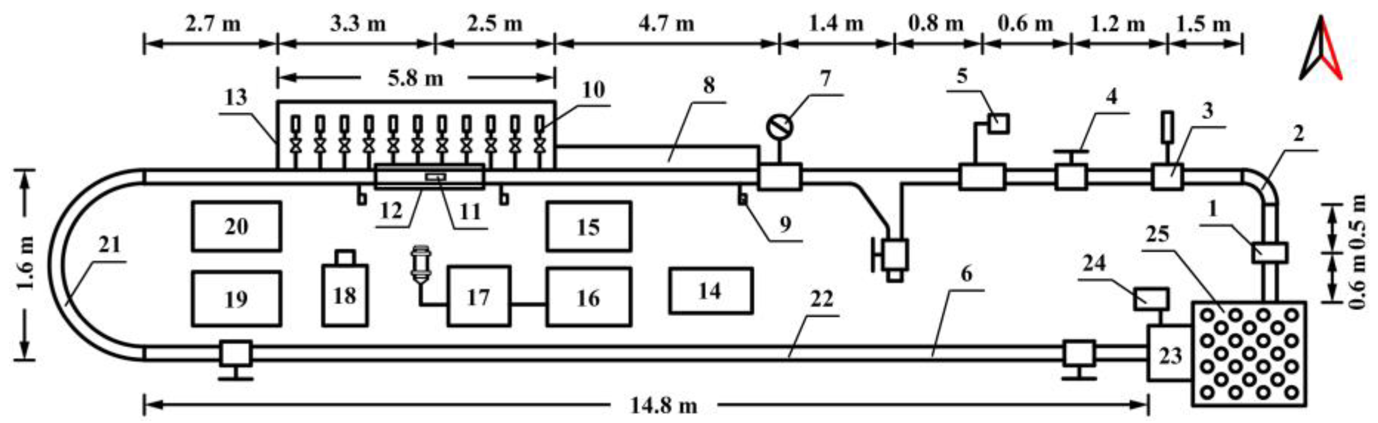
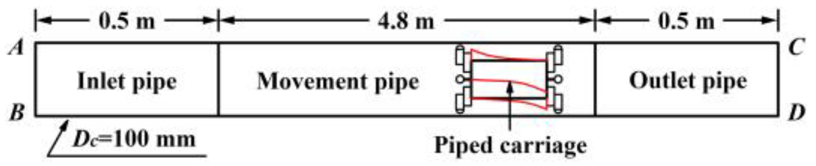
3. Materials and Methods

To verify the reliability of the simulated results from the commercial software ANSYS-Fluent 12.0 (http://www.ansys.com/Products/Fluids/ANSYS-Fluent), we conducted experimental investigations on the local hydraulic characteristics of the piped carriage transport under different placement angles of the guide vanes within the pipelines. The experimental system was located in the Fluid Dynamics Laboratory, Taiyuan University of Technology, which was composed of power devices, adjustment devices, conveying devices and dropping and receiving devices, as shown in Figure 4. The power devices included a centrifugal pumping unit and a water tank, where the rated power of the centrifugal pump motor was 15 kW at 2900 r·min⁻¹. The adjusting devices were composed of an electromagnetic flowmeter, a surge tank, several regulating valves, a braking device of the piped carriage, and a rotating control device [23]. The braking device was used to strictly control the start-up time for the piped carriage. The rotating control device was used to limit the rotary movement of the piped carriage around the center of the pipeline so that the piped carriage only had axial movement along the pipelines. The conveying devices were round Plexiglas pipes with a total length of 28.62 m and an inner diameter of 100 mm. Round flanges and rubber gaskets were used to seal and connect the different pipe sections (a horizontal pipe and a 180° pipe bend). Cast iron supports were arranged at the bottom of the conveying pipes to improve the stability of the piping system. A rectangular water channel was arranged at the Plexiglas pipelines to improve measurement precision by preventing refraction inside the pipelines of the laser beam. The dropping and receiving devices consisted of an input port for the piped carriage, an energy-eliminated orifice plate and plastic recycling bins. Sponge pads was placed on the energy-eliminated orifice plate in order to play a buffering role in emergency braking of the piped carriage. The total length of the test section was 5.8 m. 2.7 m downstream from the inlet cross-section of the 180° pipe bend and 4.7 m upstream from the braking device of the piped carriage. When the test was conducted, the water was pumped from the water tank into the steel penstocks through the centrifugal pumping unit, and the pipe discharge was adjusted to be the experimental design value through the electromagnetic flowmeter and the regulating valves. After the pipe discharge became steady, the piped carriage was first fed into the piping system through the input port of the pipe carriage. Then, the hydraulic characteristics of the internal flow field were measured by using the test instruments when the piped carriage with different guide vane placement angles moved within the horizontal pipeline. Finally, the piped carriage reached the plastic recycling bins with an aid of water thrust force. The water also flowed back to the water tank again through the pipelines, which realized circulating utilization of water. The whole experimental system formed a closed circulatory system [24].

The experimental schemes were shown in

Table 1. Experimental schemes

	Model of Piped Carriage	Model 1	Model 2	Model 3
Barrel	Length/mm	100	150	150
	Diameter/mm	70	60	70
Guide vane	Placement angle/°	3/6/9/12/15/18/21/24/27/30/33/36
	Length/mm	100	150	150
	Height/mm	10
Transport loading/kg		0.6
Pipe discharge/(m3·h−1)		50

. According to the previous published literature [38], it can be seen that the energy losses caused by the above three models of the piped carriage were relatively small. For this mentioned reasons, three types of the piped carriage were studied in this article.

Laser Doppler anemometry manufactured by the Danish company Dantech and the millisecond photoelectric timing devices (702-3A, GOOD-STAR Limited, Hong Kong, China) were used to measure the velocity distributions of the internal flow field within the pipelines. Laser Doppler anemometry was a high-precision and non-contact velocity measuring device with an error of less than 0.2%. The measurement precision of millisecond photoelectric timing devices was 0.001 s, and accurately recorded the precise time when the piped carriage passed the test section through the high- and low-level pulse signals in the system [39]. The pressure sensors (BOOST, Suzhou Xuan Sheng Medical Technology Co., Ltd., Suzhou, China) were linked to standard dynamic pressure collection system (TST5103, Chengdu test, Chengdu, China) to measure piezometric heads along the pipelines. The high-speed camera (Memrecam GX-3, NAC Image Technology, Inc., Tokyo, Japan) was connected to a personal computer via an RJ-45 connector twisted pair to measure the instantaneous axial speed and the instantaneous angular speed of the piped carriage. The high-speed camera with an image resolution of 1504 × 1280 took 500 frames every second in this article.

In this article, three typical cross-sections were selected in the test section to measure velocity distributions of the internal flow field within the pipelines, in which 1#, 2# and 3# cross-sections were 2.75, 2.85, and 2.95 m from the inlet cross-section in the test section. There were 43 velocity measurement points in the velocity test cross-sections, arranged at the intersection between seven equal spaced horizontal lines and the five equal spaced concentric annuluses. There were 12 pressure measuring points (Piezometric tubes) with an interval of 0.5 m on the right side of the horizontal wall of the test section. At the same time, the flow velocity distributions of the inlet cross-section and the pressure distributions of the outlet cross-section were measured in the test section. Measurements were made at each point three times and the average value of the measurements was reported.

The velocity data of the experimental cross-sections and the pressure data along the pipelines were analyzed statistically with Suffer 11.0, Origin 9.0, and SPSS 21.0. The two ends of the piped carriage in the flow direction were defined as the rear end (i.e., upstream end) and the front end (i.e., downstream end), respectively; these terms were important in the analysis presented in Section 6.

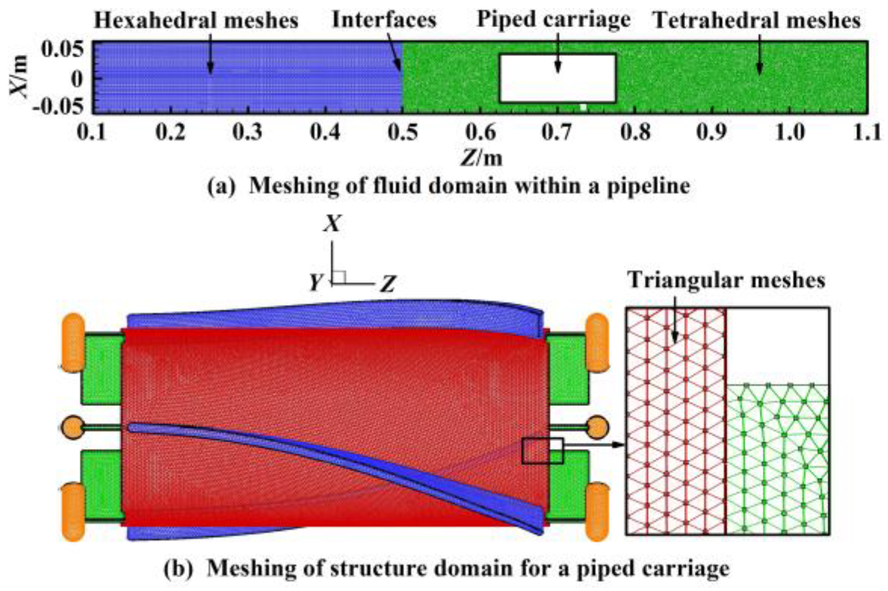
4. Bidirectional Fluid–Structure Interaction Calculation

4.1. Mathematical Model

The surface cloud data of a piped carriage was obtained by using the FARO-LDI 3D laser scanning system (Focus3D X350, FARO, Lake Mary, USA) and the mathematical model of the piped carriage transported within a horizontal pipeline was created by using the commercial software Auto CAD 2014. In order to improve the quality of the meshes, the mathematical model appropriately simplified the original model during the modeling processes. In this study, the original model was used for the numerical calculation, which can improve the calculating precision of the simulated results. The mathematical model was composed of a horizontal pipe model and a piped carriage model, as shown in Figure 5.

The horizontal pipe model was 5.8 m long with a diameter of 100 mm. The horizontal pipe model was divided into three sections: an inlet pipe, a movement pipe and an outlet pipe, where the lengths of these three sections were 0.5, 4.8, and 0.5 m respectively. The 0.5 m long inlet pipe was used in order to allow the pipe fluid to become fully developed [13]. A 0.5 m long outlet pipe can be used to reduce the effects of transporting the piped carriage on the pressure distributions of the outlet cross-section in the mathematical model. A 4.8 m long movement pipe was the scope of motion for the center of the piped carriage. The movement pipe was similar to that of Teke et al. [40], Ulusarslan et al. [28,41], and Asim et al. [30,31]. The horizontal pipe section model was identical to the size of the test section in the experimental system. In this article, three types of piped carriages were selected for the numerical calculation, exactly the same as the size of the mode testing schemes. The placement angles of the guide vanes ranged from 3 to 36° with an interval of 3°. The length of the guide vanes was the same as that of the barrel for the piped carriage, and the height of the guide vanes was 10 mm. Each support body of the piped carriage was composed of a thin cylinder and a sheet-metal plate, where the thin cylinder was 0.02 m in length and 8 mm in diameter. A 0.01 × 0.015 × 0.001 m sheet-metal plate played a significant role in connecting the barrel and the thin cylinder. The universal ball mounted at the end of the support body was a hemispherical structure with a diameter of 8 mm. In this study, the piped carriage model always maintained a concentric position with the horizontal pipe model. In the initial state, the center of the piped carriage model was 0.7 m away from the inlet cross-section in the mathematical model. The pipe discharge was 50 m³·h⁻¹ and the transport loading that consisted of the weight of the bulk solid materials only, and did not include the weight of the empty piped carriage itself was 0.6 kg. In the reference coordinate system, the center point of the inlet cross-section of the mathematical model was considered as the coordinate origin. When facing the downstream direction of the horizontal pipelines, the z-axis was defined as the direction of the water, the x-axis was defined as the direction of horizontally-left, and the y-axis was defined as the direction of vertically upward.

4.2. Governing Equations of Fluid Domain

The commercial ICEM CFD software was used to complete the meshing of the computational domain in the mathematical model. The computational domains of this article were divided into two parts: a fluid domain within the pipelines and a structural domain of the piped carriage. The fluid domain included the inlet pipe, the movement pipe, and the outlet pipe of three parts. The inlet pipe and the outlet pipe were meshed by using the structured hexahedral elements. The reason was that the structured hexahedral mesh elements can be generated in these pipes with a very low skewness and offered more accurate results due to lower numerical diffusion. In order to improve the quality of the meshes near the exterior wall of the piped carriage, the movement pipe was meshed with unstructured tetrahedral elements. The mesh density generally had great influences on the simulated results. If the number of the meshes was larger, the computing methods needed to run a long time. If the number of the meshes was less, the solving accuracy was difficult to ensure for the numerical simulation. So, it was indispensable to analyze a mesh independence test for this purpose. To reduce the effects of the mesh size on the simulated results, the mesh independence test was performed for the fluid domain in the mathematical model [42,43]. By comparing the effects of different mesh sizes on the average pressure of the inlet cross-section in the mathematical model, a reasonable mesh size was selected successfully, as shown in

Table 2. Mesh independence test

Mesh Size/m	Average Pressure of Inlet Cross-Section/Pa
	φv = 6°	φv = 12°	φv = 18°	φv = 24°	φv = 30°	φv = 36°
0.0045	11,703.21	11,606.79	11,571.42	11,518.76	11,811.74	12,111.42
0.004	11,454.86	11,369.96	11,309.38	11,323.09	11,558.04	11,888.51
0.0035	11,265.38	11,218.73	11,143.02	11,172.16	11,381.96	11,707.97
0.003	11,159.14	11,097.55	11,049.43	11,080.63	11,266.71	11,598.59
0.0025	11,101.31	11,023.58	10,967.94	11,010.39	11,201.29	11,527.81
0.002	11,057.74	10,981.52	10,922.61	10,962.48	11,158.22	11,485.09

Note: φ_v represents placement angle of a guide vane.

. The average pressure at the inlet cross-section of the mathematical model as a main indicator of the mesh independence test had the following advantages: (1) because the pressure distributions of the outlet cross-section of the pipe model were consistent, the pressure distributions of the inlet cross-section in the mathematical model can indirectly analyze the pressure drop characteristics of the mathematical model; (2) this indicator can be obtained by using the model testing, and the experimental results were used to verify the correctness of the simulated results for the pressure distributions at the inlet cross-section.

According to the simulated results of the mesh independence test in Table 2, the relative errors of the average pressure of the inlet cross-section in the mathematical model under the six different placement angles of the guide vanes were not more than 0.41% between mesh sizes of both 0.002 m and 0.0025 m. When the mesh size was less than 0.002 m, the effects of the mesh size on the average pressure of the inlet cross-section in the mathematical model were negligible. At the same time, through the comparison between the simulated results and the experimental results for the average pressure of the inlet cross-section, both results were basically consistent, and the maximum relative errors did not exceed 1.65%. When the solving accuracy and the computing efficiency were considered together, it was reasonable to use the mesh size of 0.002 m for the fluid domain of the mathematical model. In this study, local surface meshes were adopted to achieve secondary mesh refinement for the near-wall areas of the piped carriage, in which these meshes consisted of triangular elements with a specific size of 0.001 m. The velocity gradient in the near-wall areas of both the moving boundary of the piped carriage and the static boundary of the conveying pipes varied sharply. Therefore, it was necessary that the rectangular elements were adopted to mesh the boundary layer areas [44]. The thickness of the first layer in the boundary layer areas was calculated to be 0.2537 mm (y⁺ = 30) and the scale factor between two mesh layers was always 1.2. The y⁺ was the main parameter of the mesh scale in the boundary layer areas of the near-wall areas, which was the dimensionless ratio of the product of both the distance from the wall and the frictional velocity to the dynamic viscosity, which reflected the fineness of the meshes as a whole [45]. At the initial time, the meshing of both the fluid domain within the pipelines and the structural domain of the piped carriage in the mathematical model (the placement angle of the guide vanes was 24°) was shown in Figure 6.

The fluid medium in the horizontal HCPs was water with a density of 1 × 10³ kg·m⁻³ and a dynamic viscosity of 1.062 × 10⁻³ Pa·s (water temperature was 18 °C). The operating conditions being given to the solver were the operation pressure of 101,325 Pa (i.e., atmospheric pressure), and ignored the influences of the gravity on the internal flow field within the pipelines. Investigations had been carried out on the support bodies made of stainless steel having a density of 7.93 × 10³ kg·m⁻³ and the barrel made of Plexiglas having a density of 1.2 × 10³ kg·m⁻³ and the sheet-metal plate made of iron having a density of 7.78 × 10³ kg·m⁻³. Taking into account the complexity of the internal flow field caused by transport of a single piped carriage, the following assumptions must be made in the numerical calculation: (1) the physical parameters of the water were constant, thus ignoring any change of the fluid density, (2) the solving process exclude the energy equations of heat transfer, thus ignoring the frictional heat transfer between the pipe fluid and the internal wall of the conveying pipes. The continuity equation and the Reynolds time-averaged N-S equation were used in the solving process. In the Cartesian coordinates, the continuity equation and the Reynolds time-average equation for the incompressible viscous fluid in the form of a tensor index can be expressed as [46]

$$\frac{\partial \rho }{\partial t}+\frac{\partial }{\partial x_i}\left(\rho u_i\right)=0$$

(50)

$$\frac{\partial (\rho u_i)}{\partial t}+\rho \frac{\partial }{\partial x_j}(\rho u_i{u}_j)=-\frac{\partial p}{\partial x_i}+\frac{\partial }{\partial x_j}\left[\mu \frac{\partial u_i}{\partial x_j}-\rho \overline{u_i{}^{\prime }{u}_j{}^{\prime }}\right]+S$$

(51)

where t was time; u_i and u_j were the components of the time-averaged velocity in the i and j directions, respectively; $u_I^{’}$ and $u_j^{’}$ were the fluctuating velocity in the i and j directions, respectively; i and j were 1, 2, and 3, respectively. p was the time-averaged pressure; μ was the dynamic viscosity; x_i and x_j were the coordinate components in the i and j directions, respectively; S was the projection value of the generalized source term of the momentum equation in the i direction.

The criteria for internal flows (such as pipeline flows) to be turbulent that the Reynolds number was greater than 4000. It has been calculated that the flows inside the pipelines transporting the piped carriage were turbulent. Hence, a turbulent model was required to be introduced for the numerical calculation. Compared with the standard k-ε turbulent model and the Realizable k-ε turbulent model, the RNG k-ε turbulent model can better be able to deal with the multiple complicated flow problems like swirling flow, high strain rate flow, and sharply curved streamline flow. The governing equations of the RNG k-ε turbulent model [47] in the form of a tensor index can be expressed as

$$\frac{\partial \left(\rho k\right)}{\partial t}+\frac{\partial (\rho k{u}_j)}{\partial x_j}=\frac{\partial }{\partial x_j}\left({\alpha }_k{\mu }_{eff}\frac{\partial k}{\partial x_i}\right)+G_k+\rho \epsilon$$

(52)

$$\frac{\partial \left(\rho \epsilon \right)}{\partial t}+\frac{\partial \left(\rho \epsilon u_j\right)}{\partial x_j}=\frac{\partial }{\partial x_j}\left({\alpha }_{\epsilon }{\mu }_{eff}\frac{\partial \epsilon }{\partial x_i}\right)+\frac{G_k}{k}\left(C_{1\epsilon }-\frac{\eta \left(1-\eta /{\eta }_0\right)}{1+\beta {\eta }^3}\right)-C_{2\epsilon }\frac{\rho {\epsilon }^2}{k}$$

(53)

where μ_eff was the effective viscosity; G_k was the generation of turbulent kinetic energy due to the average velocity gradients; k was the turbulent kinetic energy; ε was the turbulent dissipation rate; μ_eff = μ + μ_t was the effective viscosity; μ_t = ρC_μk²/ε was turbulent viscosity, C_μ = 0.0845; C_1ε and C_2ε were the turbulent model coefficients, respectively, C_1ε = 1.42, C_2ε = 1.68; α_k and α_ε were the effective Prandtl numbers for k and ε, respectively, α_k = α_ε = 1.39; η₀ and β were constants, η₀ = 4.377, β = 0.012;

$\eta ={\left(2E_{ij}\cdot E_{ij}\right)}^{1/2}\frac{k}{\epsilon }$, $E_{ij}=\frac{1}{2}\left(\frac{\partial u_j}{\partial x_i}+\frac{\partial u_i}{\partial x_j}\right)$.

In the near-wall areas of the computational domain, the RNG k-ε turbulent model was no longer applicable due to the lower Reynolds numbers. Therefore, the standard wall function method was used for further processing and analysis at the low Reynolds numbers in the near-wall areas of the computational domain.

The following boundary conditions of the mathematical model were set as shown in

Table 3. Boundary conditions

Boundary Name	Boundary Condition
Inlet of the horizontal pipe model	Velocity Inlet
Outlet of the horizontal pipe model	Pressure Outlet
Static wall of the horizontal pipe model	Stationary Wall
Moving wall of the piped carriage	Translating Wall
Connecting cross-sections of different pipes	Interface

.

(1) The inlet boundary was set as a ‘velocity inlet’ condition. In combination with the user defined functions (UDFs), the measured velocity was used in order to define the distributions of the flow velocity at the inlet cross-section. The estimated values of Re (Reynolds number), I_c (turbulence intensity), k (turbulent kinetic energy), and ε (turbulent dissipation rate) at the inlet boundary were calculated by using the semi-empirical formulas [48]. In this study, these turbulent parameters of the pipe fluid can be expressed as

$$Re=\frac{U_{av}{D}_c}{\upsilon },I_c=0.16R{e}^{-\frac{1}{8}},k=\frac{3{\left(U_{av}\cdot I_c\right)}^2}{2},\epsilon =C_{\omega }^{0.75}\frac{k^{3/2}}{l}$$

(54)

where υ was the kinematic viscosity; l was the turbulence length scale; C_ω was the empirical constant of the turbulent model, generally taking 0.09. By calculation, the specific turbulent parameters included the Reynolds number of 166,514, the turbulence intensity of 0.035599, the turbulent kinetic energy of 0.0059446 m²·h⁻² and the turbulent dissipation rate of 0.0107589 m²·s⁻³ within the pipelines.

(2) The outlet boundary was set as a ‘pressure outlet’ condition. The measured pressure was used to define the pressure distributions at the outlet boundary of the mathematical model. Based on the measured pressure of the outlet cross-section in the mathematical model, the pressure was set to 9700 Pa.

(3) The static boundary of the horizontal pipe model was set as a ‘no-slip’ condition [30]. The conveying pipes were considered to be hydrodynamically smooth, having a wall roughness constant of zero.

(4) The moving boundary of the piped carriage was defined by using the six-degree-of-freedom (6DoF) coupling model and the UDFs in the moving mesh technology. The macro of the UDFs DEFINE SDOF PROPERTIES needed to define the moment of inertia, the rolling frictional resistance, the migration scope, and the initial state of the piped carriage.

The moment of inertia of the piped carriage [49] can be expressed as

$$J_x=J_y=\frac{1}{12}m\left(\frac{3}{4}{d}_c^2+l_c^2\right),J_z=\frac{1}{8}m{d}_c^2$$

(55)

where J_x, J_y, and J_z were the components of the moments of inertia in the three directions of x, y, and z, respectively; m was the weight of the piped carriage (including the weight of the transport loadings).

According to Equation (2), the frictional resistance was composed of the axial frictional resistance and the circumferential frictional resistance, which can be expressed as the product of the instantaneous support force of the piped carriage multiplied by the rolling frictional coefficient between the piped carriage wall and the Plexiglas pipe wall. The axial and circumferential rolling frictional resistance coefficients were obtained by experiment, and these values were set to 0.428.

Only horizontal movement along the z direction and the rotary movement around the z-axis were considered, while movement in the other directions was strictly limited. The initial instantaneous axial speed and the initial instantaneous circumferential speed of the piped carriage were defined by using the measured values of the instantaneous speed at which the center of the piped carriage passed through the corresponding cross-sections.

(5) The connecting cross-section boundaries between the inlet pipe, the movement pipe and the outlet pipe were set as ‘interface’ condition. The ‘interface’ boundaries realized mutual calling and exchange of data between the internal flow fields with the different mesh types.

In this article, the inlet cross-section and the outlet cross-section of the horizontal pipe model were set as the ‘velocity inlet’ and the ‘pressure outlet’, respectively, which were consistent with the boundary conditions that were set by Asim et al. [30,31].

The PISO velocity–pressure coupling algorithm can modify the distortion of the meshes for several times so that the deformation and reconstruction of the meshes involved in the numerical simulation can be effectively solved. At the same time, this algorithm had higher precision for solving the transient flow field. For this reason, the PISO velocity–pressure coupling algorithm was used in this article. The finite volume methods were used to discretize the governing equations of the fluid domain and reasonable relaxation factors were set to ensure the convergence speed of the simulated results [50]. The pressure terms were discretized by using a PRESTO scheme and the Reynolds stress term was discretized by using a first-order upwind scheme. The convective terms of the momentum equation, the turbulent kinetic energy equation, and the turbulent dissipation rate equation were discretized by using a second-order upwind scheme, while the diffusion terms of the above equations were discretized by using a central differencing scheme. The convergence residuals of the discrete form were set to 1 × 10⁻⁴, and the time step of the unsteady state in the numerical simulation process was 1 × 10⁻⁶ s.

4.3. Motion Equations of Structural Domain

In the 6DoF coupling model, the rigid body motion equations can solve the instantaneous speed, the instantaneous displacement and the instantaneous attitude of the piped carriage at any time. The rigid body motion equations [33,51,52] can be expressed as

$$F=m{a}_{cz},M=I{a}_{c\theta }+{\omega }_{c\theta }\times \left(I\cdot {\omega }_{c\theta }\right)$$

(56)

where F was the resultant force acting on the piped carriage; a_cz was the instantaneous accelerated speed; M was the instantaneous moment; I is the instantaneous moment of inertia matrix; V_cθ was the instantaneous angular speed; and a_cθ was the instantaneous angular acceleration. The Newmark implicit time integral method was used to solve the rigid body motion equations.

At the coupling interface between the fluid domain within the pipelines and the structural domain of the piped carriage, the mutual coupling variables such as the instantaneous displacements and instantaneous stresses of both the fluid domain and the structural domain should be equal or conserved. The conservation equations [53] can be written as

$$n{\tau }_f=n{\tau }_s,r_f=r_s$$

(57)

where τ and r were the instantaneous stress and the instantaneous displacement at the coupling surface, respectively; n was the normal vector; f was the fluid domain; s was the structural domain.

In ANSYS-Fluent 12.0, the resultant forces acting on the piped carriage consisted of the fluid loadings and the non-fluid loadings. The fluid loadings were the coupling forces that the fluids exerted on the piped carriage, including the drag and the lift, and the non-fluid loadings involved axial force and circumferential force of the rolling frictional resistance, the gravity as well as the buoyancy. The coupling forces acting on the piped carriage can be obtained by using the governing equations of the fluid domain described in Section 4.2, while the non-fluid loadings of the piped carriage needed an aided analysis of the UDFs. The gravity of the piped carriage needed to be considered in the 6DoF coupling model.

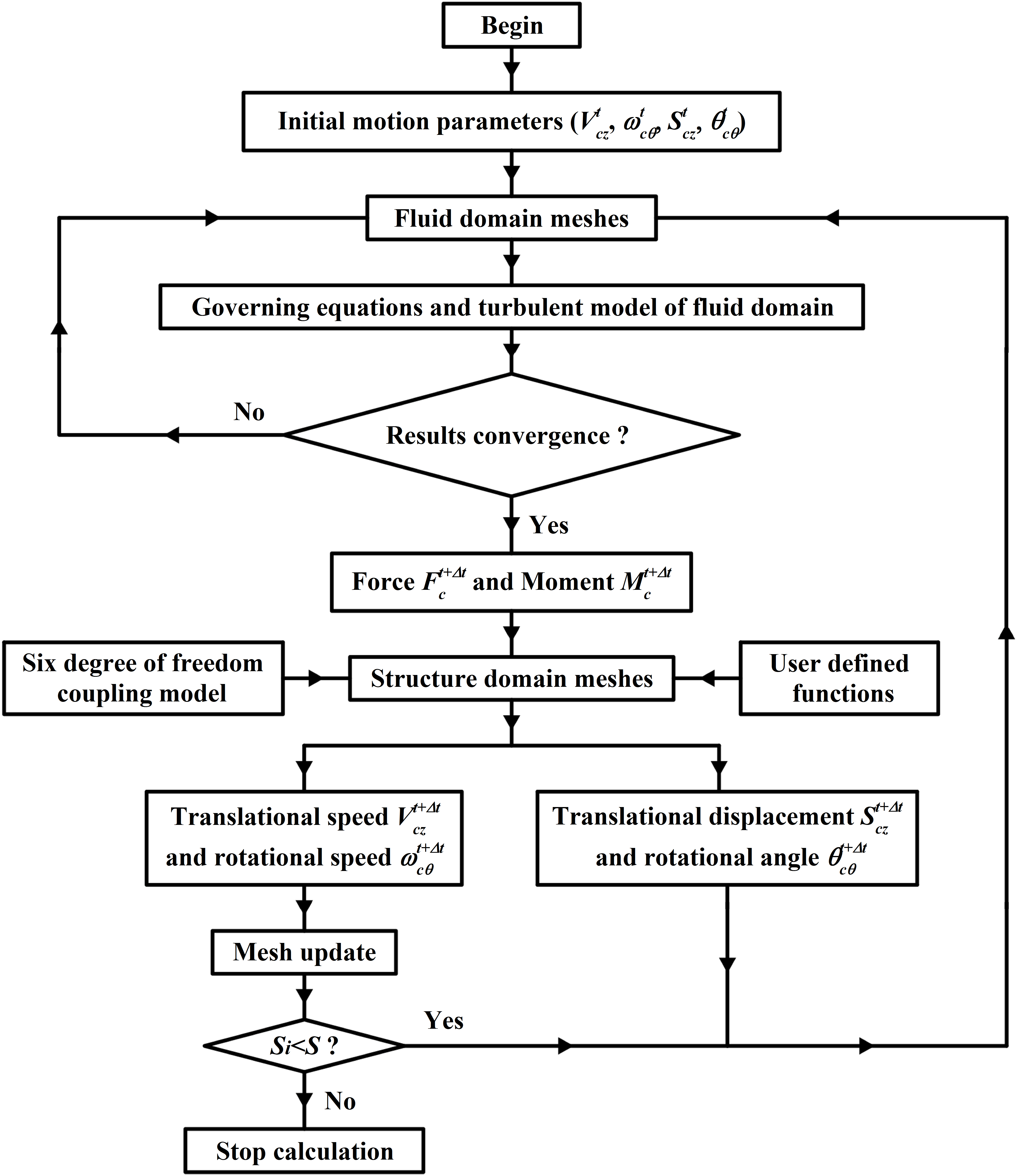
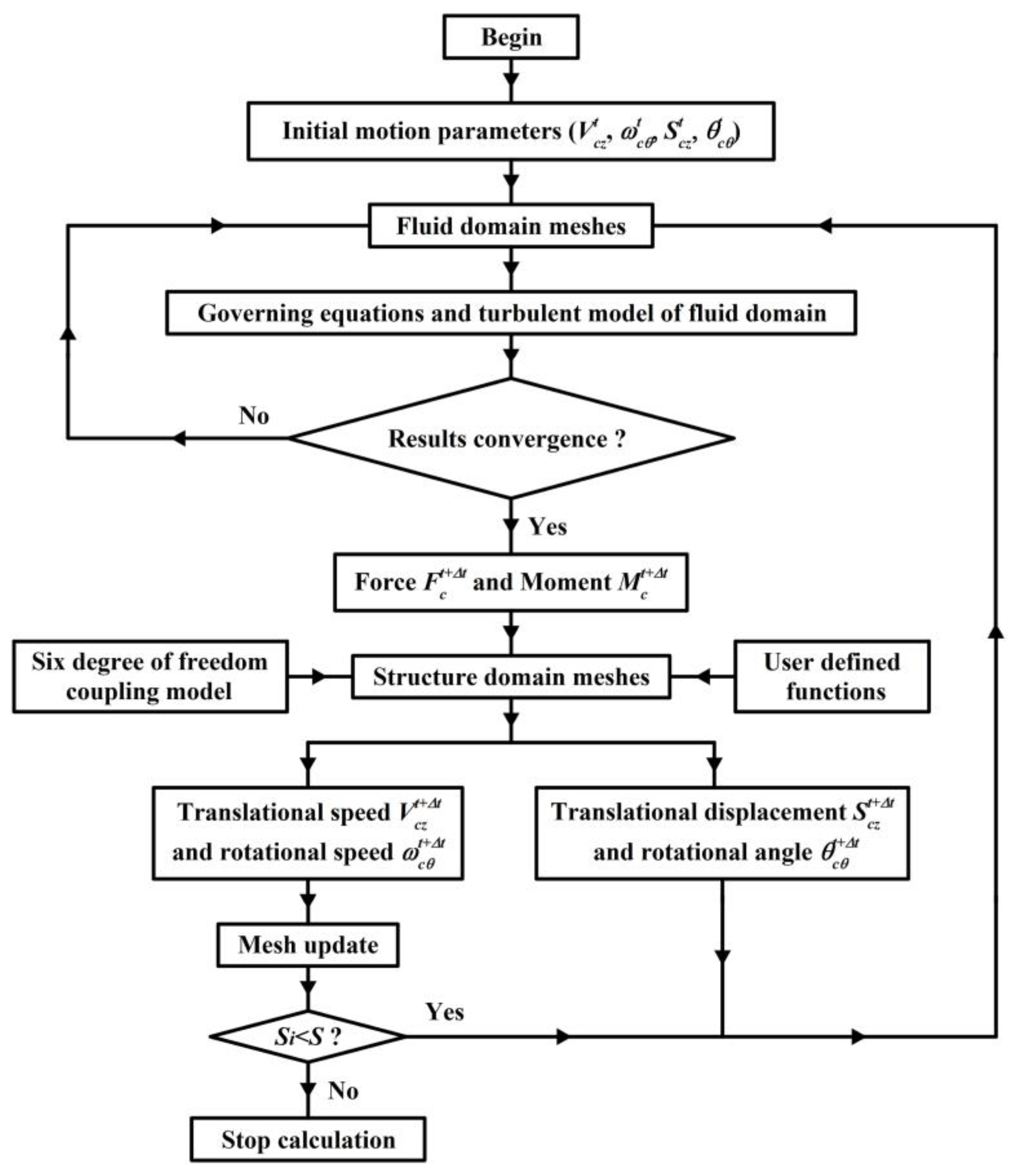
4.4. Bidirectional Fluid–Structure Interaction Algorithm

The mathematical model meshes in real time were modified by exploiting the moving mesh technology of both the elastic smoothing and the local reconstruction to adapt to the transient displacement variation caused by the coupling effects of the piped carriage [54]. Numerical investigations (non-steady state) using the RNG k-ε turbulent model were conducted on the hydraulic characteristics of the piped carriage transport within the horizontal pipelines. The 6DoF coupling model and the UDFs were used to analyze the transient dynamics responses of the single piped carriage. The coupling interface realized real-time exchange of data between the fluid domain information and the structural domain information.

The analysis process of the bidirectional fluid–structure interaction method was shown in Figure 7.

(1)

First of all, the motion parameters of the piped carriage needed to be set at the initial time t, including the instantaneous axial speed, $V_{cz}^t$; the instantaneous angular speed, ${\omega }_{c\theta }^t$; the instantaneous angle, ${\theta }_{c\theta }^t$; and the instantaneous displacement, $S_{cz}^t$.

(2)

The instantaneous axial speed and the instantaneous angular speed at time t were regarded as the boundary conditions for the next iteration. The hydraulic characteristics at time t + ∆t were solved based on the governing equations and the turbulent model of the fluid domain. When the internal flow field was fully converged, the instantaneous resultant force $F_c^{t+\Delta t}$ and the instantaneous moment $F_c^{t+\Delta t}$ acting on the piped carriage at time t + ∆t were obtained.

(3)

The instantaneous axial speed and the instantaneous displacement of the piped carriage at t + ∆t were calculated, which were expressed as

$$V_{cz}^{t+\Delta t}=V_{cz}^t+\frac{F^{t+\Delta t}}{m}\Delta t,S_{cz}^{t+\Delta t}=\frac{\left(V_{cz}^t+V_{cz}^{t+\Delta t}\right)\Delta t}{2}$$

(58)

(4)

The instantaneous angular speed and the instantaneous angle of the piped carriage at time t + ∆t were calculated, which were expressed as

$${\omega }_{c\theta }^{t+\Delta t}=\left(\frac{M}{I}-{\omega }_{c\theta }\times {\omega }_{c\theta }\right)\Delta t,{\theta }_{c\theta }^{t+\Delta t}=\frac{\left(V_{c\theta }^t+V_{c\theta }^{t+\Delta t}\right)\Delta t}{2}$$

(59)

(5)

Combined with the instantaneous displacement $S_{cz}^{t+\Delta t}$ and the instantaneous angle $V_{cz}^{t+\Delta t}$ at time t + ∆t, the piped carriage moved to a new location, and then the meshes of the fluid domain were updated by using the moving mesh technology.

(6)

The instantaneous axial speed and instantaneous angular speed at time t + ∆t were used as the boundary conditions for the next iteration. The above calculation steps were repeated again until the piped carriage arrived at the pre-defined locations in the computational domains.

5. Verification of the Simulated Results

In order to further verify the reliability of the simulated results, the simulated results were validated from three different aspects such as the instantaneous axial speed of the piped carriage, the piezometric heads through the pipelines and the axial velocity distributions of some typical cross-sections.

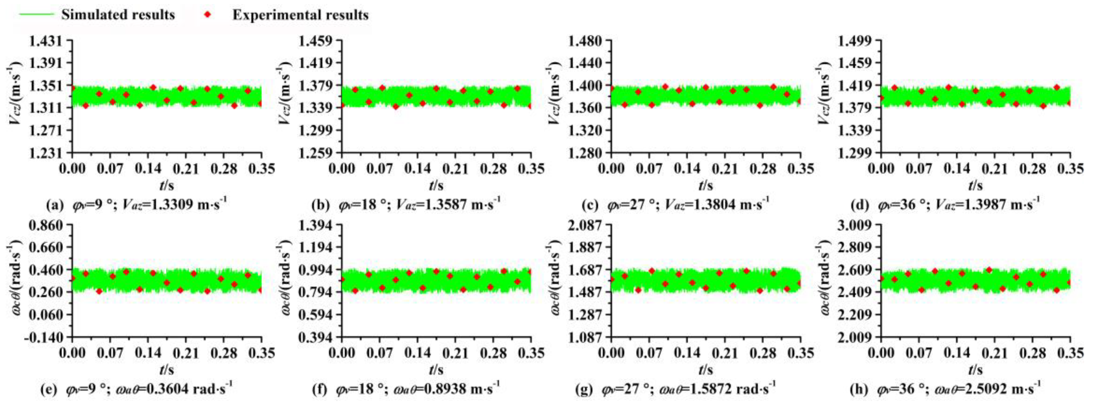
5.1. Instantaneous Speed

Figure 8 showed the comparison of the simulated results and the experimental results for both the instantaneous axial speeds and instantaneous angular speeds when the piped carriage with the four different placement angles of the guide vanes (which were 9°, 18°, 27°, and 36°, respectively) transported within the horizontal pipelines under the pipe discharge of 50 m³·h⁻¹.

The instantaneous axial speeds and the instantaneous angular speeds of the piped carriage in Figure 8 were measured by using the high-speed camera. From Figure 8a–d, the simulated results of the instantaneous axial speed of the piped carriage basically remained consistent with the experimental results, and the maximum relative errors did not exceed 3.81%. The instantaneous axial speed of the piped carriage during transport showed an irregular fluctuation within the range of ±0.02 m·s⁻¹. This appeared that the irregular fluctuation of the fluid pulsation pressure caused a fluctuating change in the instantaneous loadings that fluid acted on the piped carriage, and induced a small variation in the instantaneous acceleration of the piped carriage, resulting in the instantaneous axial speed of the piped carriage to fluctuate within a certain subtle range. Because the fluctuation range of the instantaneous axial speed was approximately two orders of magnitude less than that of the average axial speed, it was considered that the motion status of the piped carriage can be treated as a constant state. From Figure 8e–h, the simulated results of the instantaneous angular speeds of the piped carriage basically remained consistent with the experimental results, and the maximum relative errors did not more than 5.42%. The instantaneous angular speed of the piped carriage during transport showed an irregular fluctuation within the range of ±0.1 rad·s⁻¹. The reason was due to the fact that the irregular fluid pulsation pressure caused a fluctuating change in the instantaneous loadings that fluid acted on the guide vanes and led to an enormous variation of the instantaneous angular acceleration of the piped carriage, which resulted in the instantaneous angular speeds of the piped carriage to fluctuate within a certain subtle range. It can be preliminarily obtained that the piped carriage rotated around the z-axis at a constant angular speed within the pipelines.

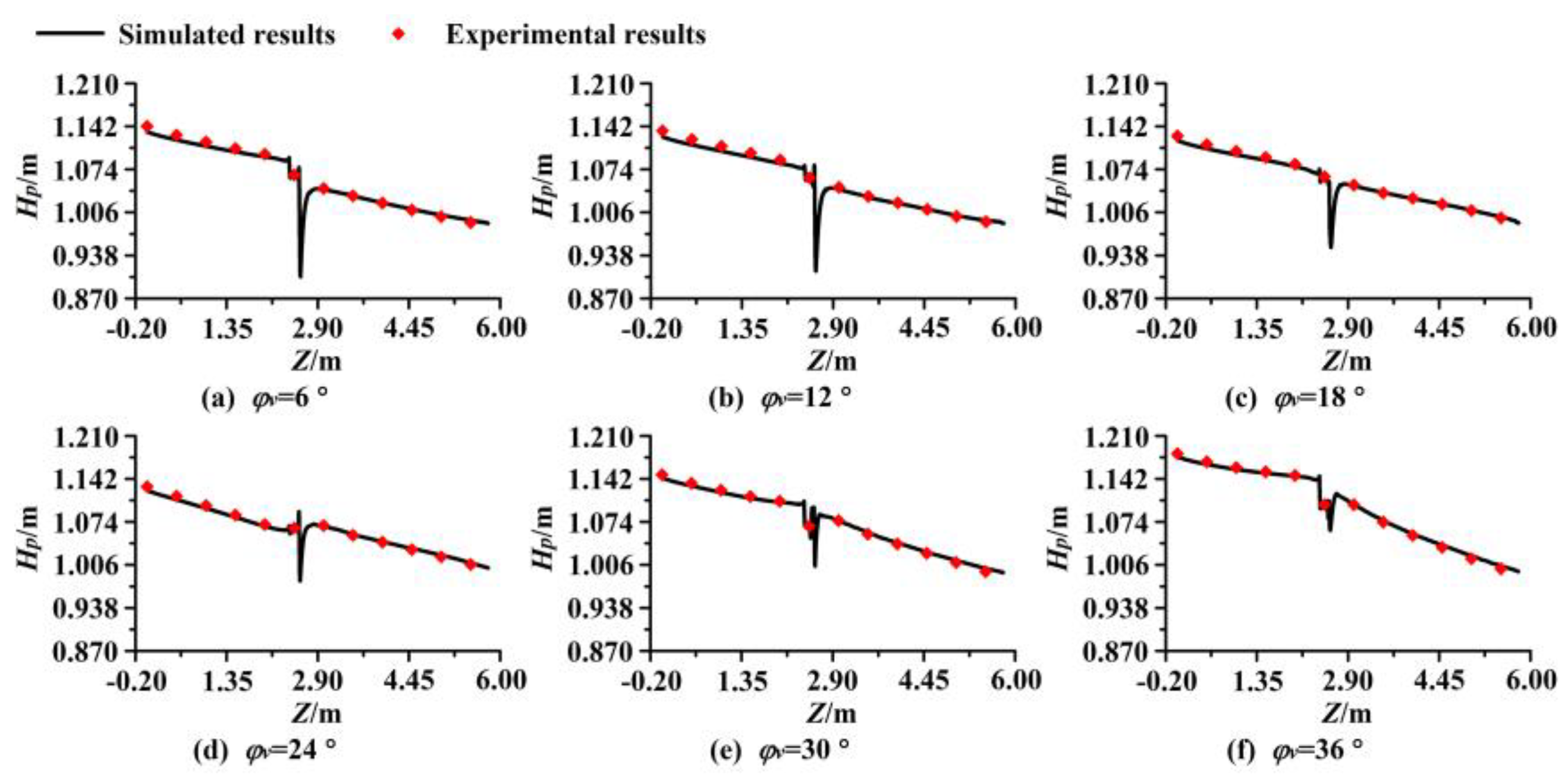
5.2. Piezometric Heads

Figure 9 showed the comparison of the simulated results and the experimental results for the piezometric heads through the pipelines when the center of the piped carriage with the six different placement angles of the guide vanes (which were 6°, 12°, 18°, 24°, 30°, and 36°, respectively) arrived at the location that was 2.5 m from the inlet cross-section of the test section under the pipe discharge of 50 m³·h⁻¹.

The pressure sensors (BOOST, Suzhou Xuan Sheng Medical Technology Co., Ltd., Suzhou, China) were used to measure the piezometric heads along the pipeline. The standard dynamic pressure collection system (TST5103, Chengdu test, Chengdu, China) was used to collect the mean piezometric heads and the pulsating piezometric heads, and transmit them to a personal computer. In order to improve the precision of the data acquiring, the acquisition frequencies of the pressure sensors was set to be 128 Hz, and the acquisition time was set to be 10 s. During a surprisingly short time, the instantaneous piezometric head was the sum of both the mean piezometric heads and the pulsating piezometric heads, and fluctuated around a mean value. This mean value was defined as the mean piezometric head. In order to improve the solving accuracy of the mean piezometric heads, the mean piezometric heads was calculated at approximately one every 0.1 s for the instantaneous pressure data of the piezometric tubes. Thereby, the variation trend of the mean piezometric heads over time was obtained. From Figure 9, it was obtained that the simulated results of the piezometric heads along the pipelines were consistent with the experimental results, and the maximum relative errors did not exceed 1.18%. As the placement angle of the guide vanes increased, the pressure drop of the piezometer heads near the front end of the piped carriage gradually decreased. This appeared because the increase of the guide vane placement angle caused an increase in the flow rate of the spiral flow in the annular slit areas towards the back-flow areas, leading to a decrease in the axial velocity in the back-flow areas. According to the flow conservation law, the axial velocity near the interior wall of the pipeline at the downstream flow field of the piped carriage gradually decreased, resulting in a decrease in the pressure drop in this region. With the increase of the guide vane placement angle, the slope of the piezometric head lines at the downstream flow field of the piped carriage gradually increased, while the slope of the piezometric head lines at the upstream flow field of the piped carriage was the same. This appeared because the increase of the guide vane placement angle caused an increase in the spiral flow intensity at the upstream flow field of the piped carriage, which led to an increase in the local energy losses of the internal flow field; thus, producing an increase in the slope of the piezometric head lines at the downstream flow field of the piped carriage with the increase of the guide vane placement angle. In addition, due to the structure of the guide vanes, the spiral flow only existed at the downstream flow field of the piped carriage; thus, the slope of the piezometric head lines at the upstream flow field of the piped carriage did not change with the increasing guide vane placement angle.

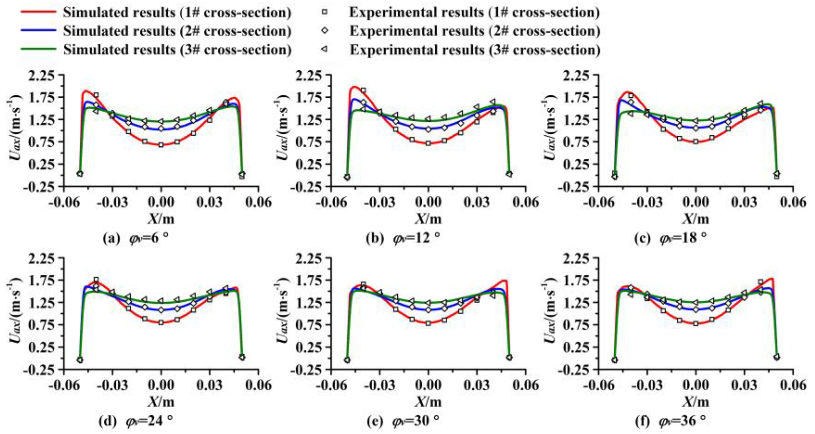
5.3. Velocity Distributions

Figure 10 showed the comparison of simulated results and experimental results for the axial velocity at the horizontal polar axis of the three different cross-sections at the downstream flow field of the piped carriage when the center of the piped carriage with the six different placement angles of the guide vanes (which were 6°, 12°, 18°, 24°, 30°, and 36°, respectively) arrived at the location that was 2.5 m from the inlet cross-section of the test section under the pipe discharge of 50 m³·h⁻¹.

Figure 10 showed the simulated results of the axial velocity at the horizontal polar axis of the three different cross-sections were consistent with the experimental results, and the maximum relative errors did not exceed 5.16%. Because the piped carriage transport had a significant impact on the velocity distributions of its downstream flow field, the simulated results of the flow velocity at the downstream flow field of the piped carriage needed to be verified. There was an obvious back-flow phenomenon near the front end of the piped carriage. The reason was due to the fact that the transition of the pipe fluid from the annular slit areas in the part where the piped carriage was to the downstream flow field of the piped carriage caused the boundary layer separation phenomenon, which led to the downstream fluid of the piped carriage gradually flowing into the cavity areas near the front end of the piped carriage. The closer the experimental cross-sections were to the front end of the piped carriage, the more obvious the back-flow phenomenon became. The reason was that the back-flow phenomenon was caused by the boundary layer separation. Therefore, the closer the experimental cross-sections were to the front end of the piped carriage, the more obvious the influences of the boundary layer separation were. Due to the effects of the guide vanes, the axial velocity distributions of the internal flow field near the front end of the piped carriage were asymmetrical. When the guide vane placement angle was 12°, the axial velocity distributions of different cross-sections in the near-wall areas of the pipeline were significantly different, and when the guide vane placement angle was 24°, the axial velocity distributions of different cross-sections in the near-wall areas of the pipeline were basically the same. The reason was due to the fact that the increasing placement angle of the guide vanes led to an increase in the flow rate of the annular slit flow flowing into the cavity areas created by the boundary layer separation so that the axial velocity of the backflow fluid diffusing towards the near-wall areas of the pipeline decreased, which led to a small change in the axial velocity gradient of different cross-sections in the near-wall areas of the pipeline. Therefore, as the placement angle of the guide vanes increased, the axial velocity distributions of different cross-sections in the near-wall areas of the pipeline were more consistent.

The numerical simulation of the bidirectional fluid–structure interaction can directly obtain the instantaneous axial speed and instantaneous angular speed of the piped carriage, which had obvious advantages by comparing with the unidirectional fluid–structure interaction method. Moreover, it was feasible to use commercial CFD software ANSYS-Fluent 12.0 to solve the hydraulic characteristics of the local flow field when the piped carriage with different placement angles of the guide vanes moved within the horizontal pipelines.

6. Results and Discussion

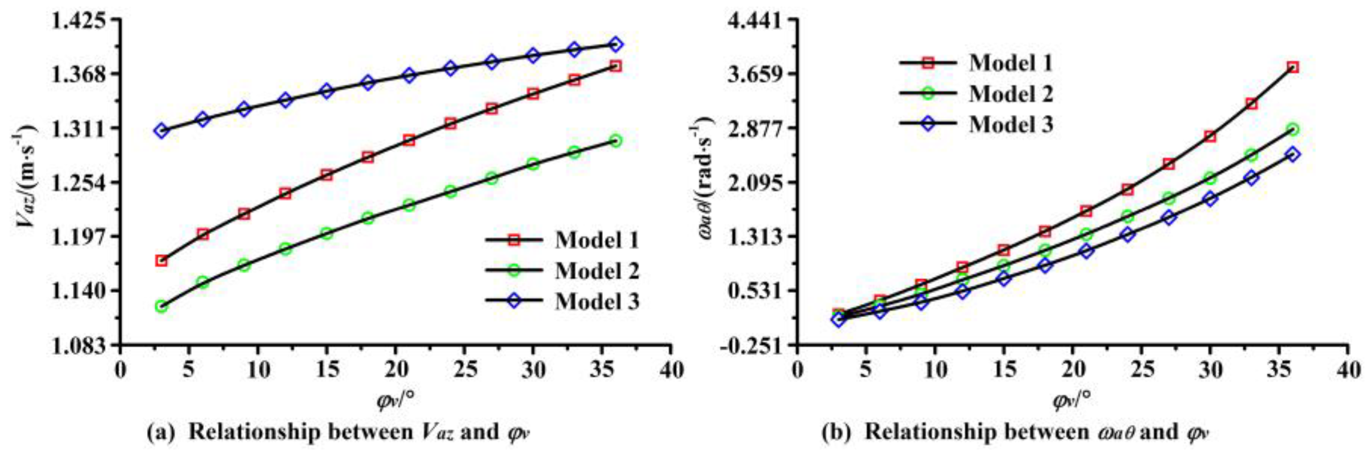
6.1. Average Speed Analysis

Figure 11 showed the changes in the average axial speeds and average angular speeds of the piped carriages as the placement angle of the guide vanes increased. From Figure 11a, it can be seen that the average axial speed of the piped carriage showed a logarithmic growth trend with the increase of the placement angle of the guide vanes. The phenomenon occurred because the increasing placement angle of the guide vanes caused an increasing axial force acting on the guide vanes under the action of the pipe fluid, resulting in an increase in the average axial speed of the piped carriage. The increase in the diameter and the length of the piped carriage caused a gradual increase in the buoyancy acting on the piped carriage, which led to a decrease in the frictional resistance. The greater the diameter of the piped carriage was, the larger the pressure gradient force that fluid acted on the piped carriage was. The greater the length of the piped carriage was, the greater the shear stress that fluid acted on the sidewall of the piped carriage was. Because the shear stress was significantly smaller than the pressure gradient force for the piped carriage, the Model 3 of piped carriage had the largest average axial speed, and Model 1 of the piped carriage was the second, and Model 2 of the piped carriage was the smallest. According to Equation (30), the average axial velocity of the piped carriage can be qualitatively analyzed. The increase of the guide vane placement angle caused growth rate of the C₁ to be larger than that of the B₁ so that the symmetry axis of the equation gradually increased, which led to an increase in the abscissa of the intersection point between the equation and the x-axis. Therefore, the average axial speed of the piped carriage gradually increased with increasing placement angle of guide vanes. From Figure 11b, it can be seen that the average angular speed of the piped carriage increased exponentially as the placement angle of the guide vanes increased. The phenomenon occurred because the increase of the placement angle caused an increase in the reverse resistance and the circumferential force acting on the piped carriage, resulting in an increase in the average angular speed of the piped carriage. From Equation (49) in Section 2.4, it can also be found that the increase of the guide vane placement angle caused a logarithmic growth of sinφ_v, resulting in a logarithmic increase in the average angular speed. When the placement angles of the guide vanes were the same, the closer the relative velocity between the piped carriage and the pipe fluid was, the smaller the average angular speed of the piped carriage was. Therefore, the Model 2 of the piped carriage had the largest average angular speed, the Model 1 of the piped carriage was the second, and the Model 3 of the piped carriage was the lowest. According to Equation (55), the rotational torque of the Model 3 of the piped carriage was the smallest, which further explained that the average angular velocity of the Model 3 of the piped carriage was the largest.

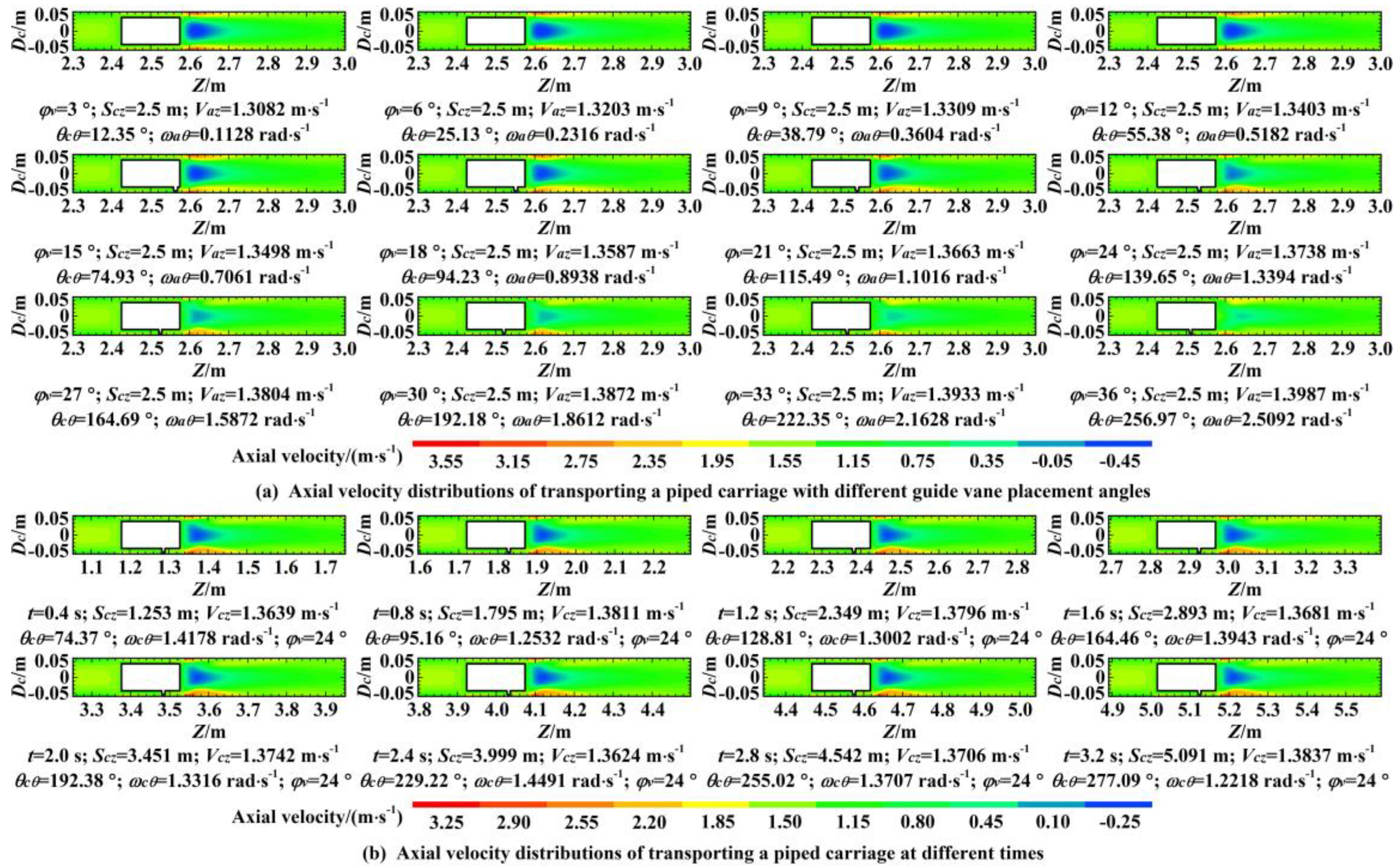
6.2. Axial Velocity Distributions

Figure 12a showed the axial velocity distributions of the internal flow field within the pipelines when the center of the piped carriage with the different placement angles of the guide vanes arrived at the location that was 2.5 m away from the inlet cross-section of the test section under the pipe discharge of 50 m³·h⁻¹. For the sake of contrastive analysis of the internal flow field characteristics, all the flow field distributions of the center cross-sections in Section 6 were selected to be perpendicular to the support bodies.

As shown in Figure 12a, the obvious back-flow areas existed near the front end of the piped carriage. The phenomenon occurred because there was the adverse pressure gradient existed in the boundary layer of the piped carriage wall, which resulted in the boundary layer separation in the annular slit areas of the front end of the piped carriage. As a result, the annular slit flow leaved the front end of the piped carriage and its downstream fluid randomly flowed into the cavity areas formed by the boundary layer separation. There were two high velocity areas at the entrance location of the annular slit flow and in the near-wall areas of the pipeline at the downstream flow field of the piped carriage. The reason why the high velocity areas at the entrance location of the annular slit flow were generated was that the boundary layer separation caused a decrease in the main cross-section areas so that the axial velocity at these areas increased. The high velocity areas in the near-wall areas of the pipeline at the downstream flow field of the piped carriage were formed by the interaction of the back-flow fluid with the front end of the piped carriage, resulting in high-speed diffusion of the back-flow fluid towards the near-wall of the conveying pipes. In addition, due to the influences of the guide vanes, the distributions of the high axial velocity areas were asymmetrically at the downstream flow field of the piped carriage. As the placement angle of the guide vanes increased, the affected range in the axial velocity of the back-flow areas at the downstream flow field of the piped carriage gradually decreased. These results occurred such that the increasing placement angle of the guide vanes led to an increase in the flow rate of the annular slit flow flowing into the cavity areas created by the boundary layer separation, thus resulting in a decrease in the affected range in the axial velocity of the back-flow areas. With the increase of the placement angle of the guide vanes, the axial velocity of the high velocity areas near wall of the conveying pipes at the downstream flow field of the piped carriage gradually decreased. This was mainly due to that fact that the decreasing axial velocity in the back-flow areas caused a decrease in the relative velocity between the back-flow fluid and the piped carriage, resulting in a decrease in the axial velocity that diffused towards the near-wall areas at the downstream flow field of the piped carriage.

Figure 12b showed the axial velocity distributions of transporting a piped carriage having a guide vane placement angle of 24° at different time under the pipe discharge of 50 m³·h⁻¹.

Due to the interaction between the piped carriage and the pipe fluid, the axial velocity in the near-wall areas of the piped carriage appeared to be unsteady. As shown in Figure 12b axial velocity distributions in the near-wall areas of the piped carriage were basically the same at different times, and there was no periodic variation of the axial velocity distributions over time. The difference between the maximum axial velocity and the average maximum axial velocity was not more than 1.53%. These results occurred because the instantaneous axial speed and instantaneous angular speed changed with a limited range, leading to the uniform axial velocity distributions of the bidirectional interaction system formed by both the piped carriage and the pipe fluid at any time.

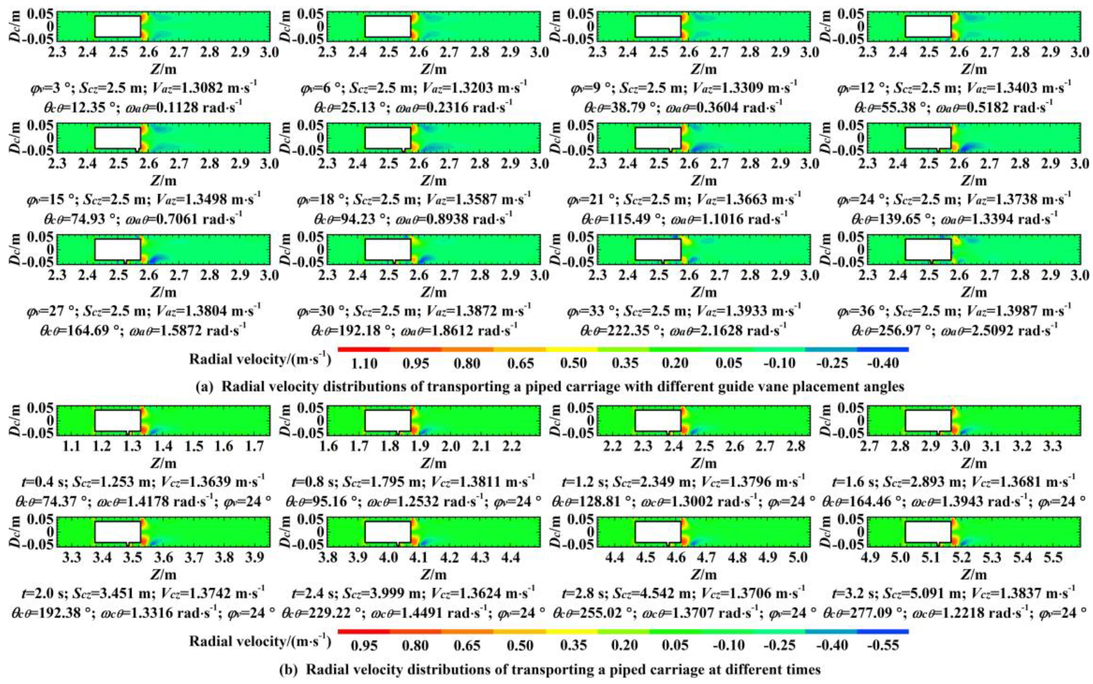
6.3. Radial Velocity Distribution

Figure 13a showed the radial velocity distributions of the internal flow field within the pipelines when the center of the piped carriage with the different placement angles of the guide vanes arrived at the location that was 2.5 m away from the inlet cross-section of the test section under the pipe discharge of 50 m³·h⁻¹.

From Figure 13a, the radial velocity of the internal flow field within the pipelines was mainly distributed near the front and rear ends of the piped carriage, and the direction of the radial flow velocity was directed from the center of the pipe to the pipe internal wall. This phenomenon appeared because the forming principles of the radial velocity near the front and rear ends of the piped carriage were different. For the radial velocity near the rear end of the piped carriage, the reason was that the pipe fluid affected by the rear end of the piped carriage shrank into the annular slit areas, which caused radial velocity flowing from the center of the pipe to the wall of the pipe. As for the radial flow velocity near the front end of the piped carriage, the reason was due to the fact that the pipe fluids in the back-flow areas and the front end of the piped carriage interacted with each other, which led to the radial velocity dispersed from the center of the pipe to the wall of the pipe. The greater the relative velocity between the pipe fluid and the piped carriage was, the larger the radial velocity of the internal flow field was. Because of the higher relatively relative velocity between the back-flow fluid and the front end of the piped carriage, the radial velocity of the internal flow field near the front end of the piped carriage was greater. The radial velocity at the downstream flow field of the piped carriage was smaller, and the direction of the radial velocity pointed to the center of the pipe from the pipe wall; this area was formed by the diffusion of the annular slit flow towards the downstream flow field of the piped carriage. As the placement angle of the guide vanes increased, the affected areas of the radial velocity near the front and rear ends of the piped carriage gradually decreased. These results occurred because as the placement angle of the guide vane increased, the decreasing relative velocity between the rear end of the piped carriage and the pipe fluid caused a decrease in the affected areas of the radial velocity near the rear end of the piped carriage. In addition, the decreasing relative velocity between the front end of the piped carriage and the back-flow fluid decreased the areas of affected radial velocity near the front end of the piped carriage.

Figure 13b showed the radial velocity distributions of transporting a piped carriage having a guide vane placement angle of 24° at different time under the pipe discharge of 50 m³·h⁻¹.

Due to the interaction between the piped carriage and the pipe fluid, the radial velocity in the near-wall areas of the piped carriage appeared to be unsteady. As shown in Figure 13b radial velocity distributions in the near-wall areas of the piped carriage were basically the same at different times, and there was no periodic variation of the radial velocity distributions over time. The difference between the maximum radial velocity and the average maximum radial velocity did not more than 2.09%. These results occurred because the instantaneous axial speed and instantaneous angular speed changed with a limited range, leading to the uniform radial velocity distributions of the bidirectional interaction system formed by both the piped carriage and the pipe fluid at any time.

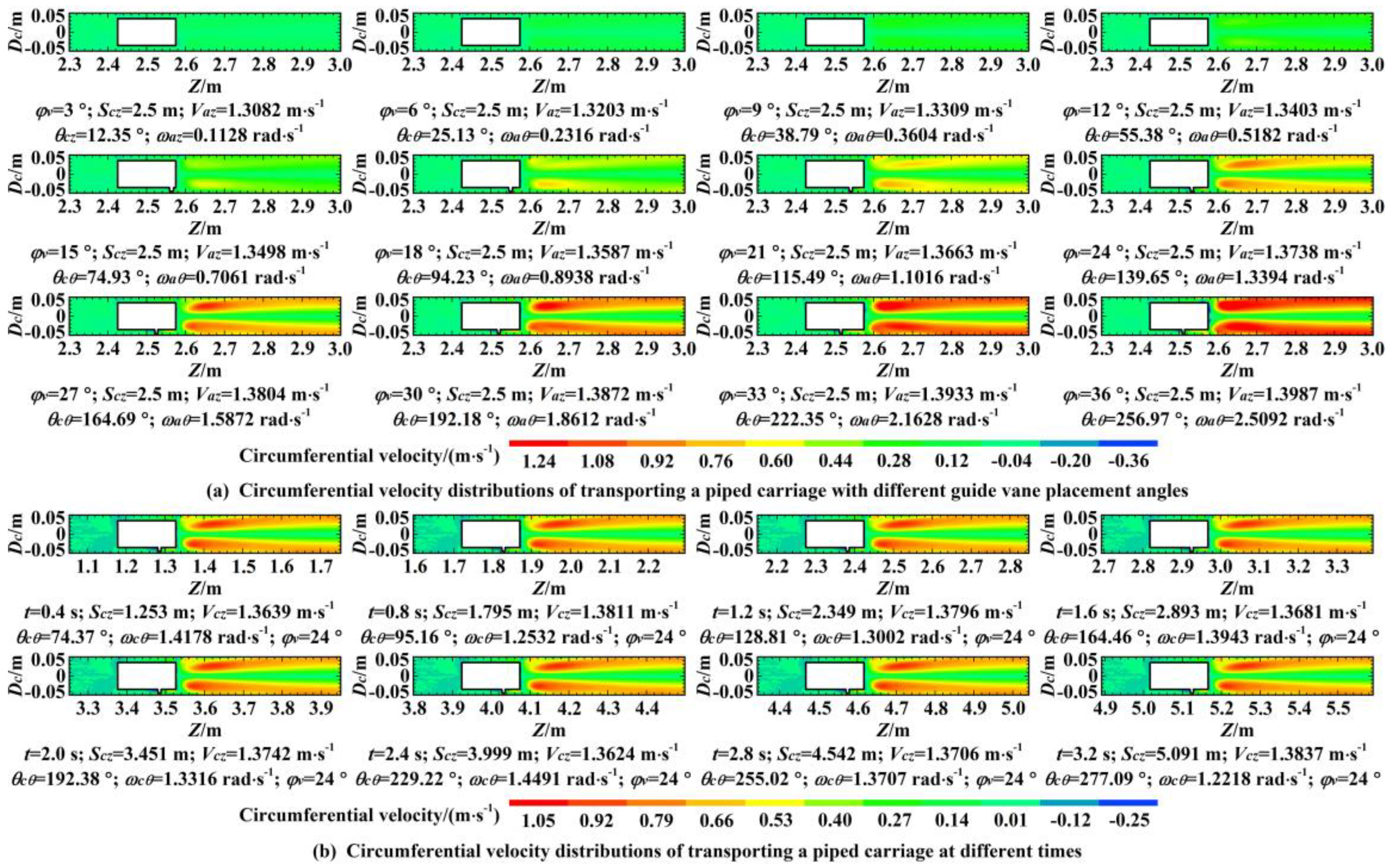
6.4. Circumferential Velocity Distribution

Figure 14a showed the circumferential velocity distributions of the internal flow field within the pipelines when the center of the piped carriage with the different placement angles of the guide vanes arrived at the location that was 2.5 m away from the inlet cross-section of the test section under the pipe discharge of 50 m³·h⁻¹.

From Figure 14a, the circumferential velocity near the rear end of the piped carriage was caused by the support bodies, therefore the maximum circumferential velocity appeared near the wall of the support bodies. Under the action of the pipe fluid, the front end of the piped carriage rotated clockwise. This variation occurred because the pipe fluid had a certain viscosity, the circumferential velocity near the front end of the piped carriage presented clockwise. Because the twisting direction of the guide vanes rotated counterclockwise from the rear end of the piped carriage to its front end, the circumferential velocity near the front end of the piped carriage was in the clockwise direction. There were larger circumferential velocity distributions near the wall of the guide vanes in the annular slit areas. This was due to the fact that two forces of both the reverse resistance and the vertical lift generated by the fluid acting on the guide vanes caused a large degree of curvature of the streamlines near the wall of the guide vanes, resulting in the formation of a spiral flow with uniform intensity of vorticity within the pipelines. The circumferential velocity at the downstream flow field of the piped carriage was formed by the diffusion of the spiral flow in the annular slit areas towards its downstream flow field. As the placement angle of the guide vanes increased, the circumferential velocity and the affected areas at the downstream flow field of the piped carriage gradually increased. This variation occurred because the increase of the placement angle of the guide vanes caused an increase in the curvature of the streamlines at the downstream flow field of the piped carriage, resulting in the increase of the velocity circulation formed within the pipelines. Since the average angular speed of the piped carriage gradually increased with the increase of the placement angle of the guide vanes, the circumferential velocity near the front end of the piped carriage gradually showed a trend of increasing with the increase of the placement angle of the guide vanes. When the piped carriage travelled through the horizontal pipelines, the obvious areas of circumferential velocity distributions were developed at the downstream flow field of the piped carriage. The hydraulic characteristics of transporting the piped carriage were distinguished from that of transporting the carriers in the published literature. Asim et al.’s [30] studies found that significant circumferential velocity distributions were not formed at the downstream flow field of the cylindrical capsule, when the cylindrical capsule moved inside the pipelines.

Figure 14b showed the circumferential velocity distributions of transporting a piped carriage having a guide vane placement angle of 24° at different time under the pipe discharge of 50 m³·h⁻¹.

Due to the interaction between the piped carriage and the pipe fluid, the circumferential velocity in the near-wall areas of the piped carriage appeared to be unsteady. As shown in Figure 14b circumferential velocity distributions in the near-wall areas of the piped carriage were basically the same at different times, and there was no periodic variation of the circumferential velocity distributions over time. The difference between the maximum circumferential velocity and the average maximum circumferential velocity did not more than 1.75%. These results occurred because the instantaneous axial speed and instantaneous angular speed changed with a limited range, leading to the uniform circumferential velocity distributions of the bidirectional interaction system formed by both the piped carriage and the pipe fluid at any time.

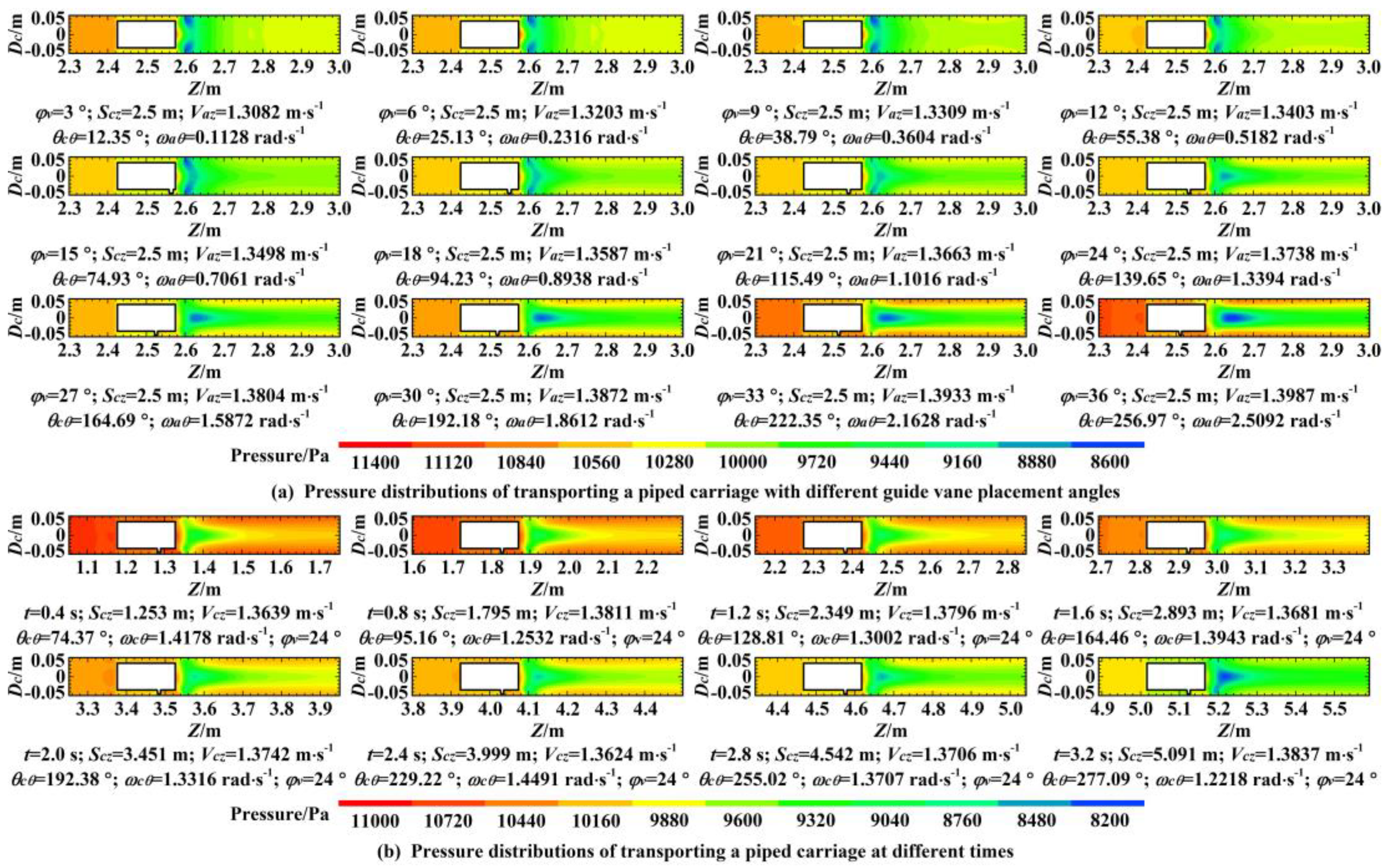
6.5. Pressure Distributions

Figure 15a showed the pressure distributions of the internal flow field within the pipelines when the center of the piped carriage with the different placement angles of the guide vanes arrived at the location that was 2.5 m away from the inlet cross-section of the test section under the pipe discharge of 50 m³·h⁻¹.

From Figure 15a, the local high-pressure areas of the internal flow field existed near the front and rear ends of the piped carriage within the pipelines. This phenomenon appeared for different reasons at the front and rear ends of the piped carriage. Considering the high-pressure areas near the rear end of the piped carriage, the reason was that the fluid kinetic energy was converted into pressure energy under the action of the piped carriage. As for the high-pressure areas near the front end of the piped carriage, the reason was due to fact that collision between the back-flow fluid and the piped carriage caused the fluid kinetic energy to be converted into pressure energy. The greater the relative velocity between the pipe fluid and the piped carriage was, the greater the local pressure growth was; thus, the growth rate of the pressure near the front end of the piped carriage had been obviously higher than that near the rear end. The obvious low-pressure areas at the downstream flow field of the piped carriage were developed, and the pressure at the downstream flow field of this areas gradually rose again. This reason was due to the fact that mixing between the annular slit flow and the downstream fluid of the piped carriage caused two processes such as energy dissipation and energy conversion. The energy dissipation was the process of converting kinetic energy into internal energy due to the viscosity of the fluid when the downstream fluid interacted with the annular slit flow. Simultaneously, the energy conversion was the process of converting the kinetic energy into the pressure energy of the downstream fluid when the annular slit flow collided with the downstream fluid of the piped carriage. The dual effects of both the energy dissipation and the energy conversion together caused the distinct low-pressure areas at the downstream flow field of the piped carriage, while the energy conversion caused the pressure to rise again at the downstream flow field of these low-pressure areas. With the increase of the placement angle of the guide vanes, the scope of the high-pressure areas near the front and rear ends of the piped carriage gradually decreased. This behavior occurred for different reasons near the front and rear of the piped carriage. The reason for the high-pressure areas near the rear end of the piped carriage was that the increase of the placement angular of the guide vanes caused a decrease in the relative velocity between the piped carriage and its upstream fluid, resulting in a decrease in the degree to which kinetic energy was converted into pressure energy. Meanwhile, the reason why the high-pressure areas near the front end of the piped carriage were generated was that the flow velocity of the back-flow fluid under the action of the guide vanes gradually decreased with increasing the placement angle of the guide vanes, resulting in a decrease in the high pressure areas near the front end of the piped carriage. With the increase of the placement angle, the pressure drop at the downstream flow field of the piped carriage became more severe. The reason was that the spiral flow intensity in the annular slit areas gradually increased with the increase of the guide vane placement angle, resulting in severe energy dissipation at the downstream flow field of the piped carriage. The pressure at the upstream flow field of the piped carriage showed a trend of decrease first and then increase. This occurred because the energy losses caused by transporting the piped carriage decreased first and then increased with the increase of the guide vane placement angle. This is described in detail in Section 6.7.

Figure 15b showed the pressure distributions of transporting a piped carriage having a guide vane placement angle of 24° at different time under the pipe discharge of 50 m³·h⁻¹.

From Figure 15b, the pressure in the near-wall areas of the piped carriage showed an overall decreasing trend over time. This occurred because the instantaneous axial speed and instantaneous angular speed changed within a limited range when the piped carriage transported along the horizontal pipelines, which led to the same energy losses of transporting the piped carriage at different times. Because the pressure inside the pipeline gradually decreased, the pressure in the near-wall areas of the piped carriage reduced when the piped carriage moved towards the downstream flow field of the conveying pipes.

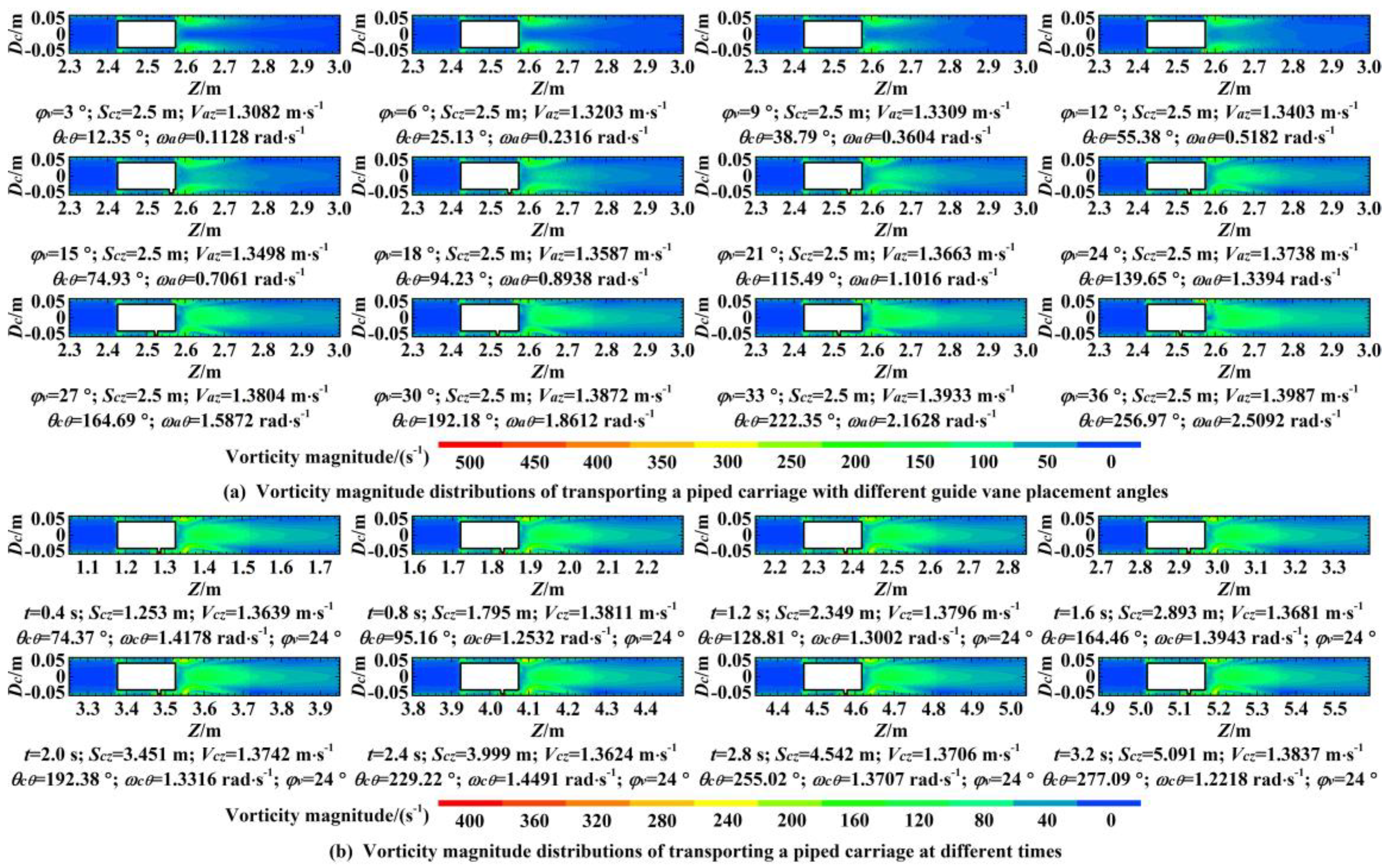
6.6. Vorticity Magnitude Distributions

Figure 16a showed the vorticity magnitude distributions of the internal flow field within the pipelines when the center of the piped carriage with the different placement angles of the guide vanes arrived at the location that was 2.5 m away from the inlet cross-section of the test section under the pipe discharge of 50 m³·h⁻¹.

From Figure 16a, the vorticity magnitude distributions of the internal flow field within the pipelines were mainly distributed near the rear sidewall of the barrel, in the near-wall areas of the guide vanes and at the interface between the annular slit flow and the downstream fluid of the piped carriage. When the piped carriage moved within the pipelines, the boundary layer separation near the rear sidewall of the barrel formed a local vortex, which in turn caused the distinct vorticity magnitude distributions. The reverse resistance and the vertical lift generated by the guide vanes under the action of the pipe fluid caused a large degree of curvature of the streamlines, which led to forming a vortex with uniform intensity of vorticity. The annular slit flow was mixed with the downstream fluid of the piped carriage, which caused the formation of the obvious vorticity magnitude at their interface between two fluids. The vorticity magnitude at the entrance location was greater than that at the exit location for the annular slit areas. The reason for the formation of the vorticity magnitude at entrance location was that the pipe fluid suddenly contracted near the rear end of the piped carriage, and the annular slit flow at the boundary of the piped carriage produced an enormous boundary layer separation. In addition, the vorticity magnitude at the exit location was caused by the disturbance of the guide vanes to the annular slit flow. Due to the greater degree of curvature of the streamlines caused by the boundary layer separation at entrance location of the annular slit areas, the vorticity magnitude in these areas was larger. With the increase of the guide vane placement angle, the vorticity magnitude near the rear end of the piped carriage was gradually reduced, while the vorticity magnitude at the downstream flow field of the piped carriage was gradually increased. This behavior occurred for different reasons. The vorticity magnitude near the rear end of the piped carriage appeared because the increasing placement angle of the guide vanes caused a decrease in the relative velocity between the piped carriage and pipe fluid, leading to a drastic reduction in affected scope of the boundary layer separation. However, the vorticity magnitude at the downstream flow field of the piped carriage appeared because the increase of the placement angle of the guide vanes caused an increase in the circumferential velocity of the annular slit flow and caused a serious blending between the annular slit flow and the downstream fluid of the piped carriage, resulting in an increase in the vorticity magnitude at the downstream flow field of the piped carriage. With the increase of the placement angle of the guide vanes, the affected areas of the vorticity magnitude at the downstream flow field of the piped carriage gradually increased. This appeared because as the placement angle of the guide vanes increased, the back-flow areas existed near the front end of the piped carriage gradually decreased; thus producing an increase in spreading scope of the vorticity magnitude towards the downstream flow field of the piped carriage.

Figure 16b showed the vorticity magnitude distributions of transporting a piped carriage having a guide vane placement angle of 24° at different time under the pipe discharge of 50 m³·h⁻¹.

Due to the interaction between the piped carriage and the pipe fluid, the vorticity magnitude in the near-wall areas of the piped carriage appeared to be unsteady. As shown in Figure 16b vorticity magnitude distributions in the near-wall areas of the piped carriage were basically the same at different times, and there was no periodic variation of the vorticity magnitude distributions over time. The difference between the maximum vorticity magnitude and the average maximum vorticity magnitude did not more than 1.84%. These results occurred because the instantaneous axial speed and instantaneous angular speed changed with a limited range, leading to the uniform vorticity magnitude distributions of the bidirectional interaction system formed by both the piped carriage and the pipe fluid at any time.

6.7. Pressure Drop Characteristics

Figure 17 showed the trend of the average pressure drop coefficient with the increase of the guide vane placement angle under the pipe discharge of 50 m³·h⁻¹, when the three types of the piped carriage moved along the horizontal pipelines.

The energy losses of the piped carriage transport were represented by using the pressure drop coefficient. The pressure drop coefficient was the ratio of the total pressure drop for the piped carriage flow to the total pressure drop that would exist if fluid alone flowed in the same conveying pipes at the same average velocity. Due to the effects of the fluid pulsation pressure, the pressure drop coefficient of the piping system fluctuated irregularly over time. For this reason, the average pressure drop coefficient was used to analyze the energy losses of transporting the piped carriage. Therefore, the average pressure drop coefficient can be expressed as

$$C_p=\frac{\Delta P_m}{\Delta P_n}$$

(60)

where ∆P_m was the total pressure drop for the piped carriage flow; ∆P_n was the total pressure drop that would exist if fluid alone flowed in the same pipe at the same average axial velocity.

With the increasing placement angle of the guide vanes, the average pressure drop coefficient of the piped carriage decreased first and then increased, and the average pressure drop coefficient caused by transporting the piped carriage with guide vane placement angle of 21° was the smallest. According to the change laws of the above curves in Figure 17, it can be founded that when the guide vane placement angle was less than 21°, the average axial speed of the piped carriage played a dominant role such that the increasing speed of the piped carriage decreased the local energy losses. When the guide vane placement angle was greater than 21°, the placement angles of the guide vanes became the main affecting factor, which led to an increase in the energy losses with the increase of the placement angle of the guide vanes. The Model 3 of the piped carriage had the lowest average pressure drop coefficient, the Model 1 of the piped carriage was the second, and the Model 2 of the piped carriage was the highest. This phenomenon appeared because the guide vanes of Model 2 has the largest distortion angle and the lowest average axial speed, so the average pressure drop coefficient caused by this model of the piped carriage was the largest. Simultaneously, the increasing average axial speed of the piped carriage decreased the average pressure drop coefficient. Therefore, the average pressure drop coefficient for the Model 3 of the piped carriage was the lowest.

6.8. Mechanical Efficiencies

Mechanical efficiency was one of the important indicators to evaluate the performance of the mechanical properties. Mechanical efficiency denoted the transformation efficiency with which the total energy of the pipe fluid was changed into mechanical energy for the piped carriage transport in physics. The total energy of the pipe fluid represented the total energy losses of the pipe fluid around the piped carriage, and the mechanical energy represented the kinetic energy of the piped carriage. The mechanical efficiency was defined as the ratio of the average kinetic energy of the piped carriage to the average total energy losses of the pipe fluid around the piped carriage, which can be expressed as

$$\eta =\frac{F_d{V}_{az}}{A_p{U}_{av}\rho g\left(\Delta P_m-\Delta P_n\right)}\times 100\%$$

(61)

where η was the mechanical efficiency; A_p was the pipe cross-sectional areas.

Figure 18 showed the variation trend of the mechanical efficiency of the piped carriage as the guide vane placement angle increased when the piped carriage moved within the pipelines. As shown in Figure 18, with the increase of the placement angle of the guide vanes, the mechanical efficiency of the piped carriage first increased and then decreased clearly. The mechanical efficiency of transporting the piped carriage with guide vane placement angle of 21° was the highest within the pipelines, and reached its maximum value of 85.3%; thus, this higher efficiency sufficiently showed that the piped carriage had a higher transport efficiency than other transport modes. The mechanical efficiency for Model 3 of the piped carriage was the highest, Model 1 of the piped carriage was the second, and Model 2 of the piped carriage was the lowest. The mechanical efficiency for Model 3 of piped carriage was the highest because it had the largest kinetic energy and the smallest total energy losses of the pipe fluid around the piped carriage, while the mechanical efficiency for Model 2 of piped carriage was the lowest because it had the smallest kinetic energy and the largest total energy losses of the pipe fluid around the piped carriage. When the guide vane placement angle was 21°, the mechanical efficiency of the piped carriage in HCPs reached the maximum value. The above conclusions were suitable for the special case in which the pipe discharge was 50 m³·h⁻¹ and the transport loading was 0.6 kg.

6.9. Force Statistics

Figure 19 showed the variation trend of the force statistics of the piped carriage with the increase of the guide vane placement angle. The drag coefficient was the ratio of the drag of the piped carriage to the product of both the hydrodynamic pressure of the fluid and the reference areas which were perpendicular to the pipe flow. Because the drag coefficient of the piped carriage transport within the pipelines changed irregularly over time, the average drag coefficient was used to analyze the drag characteristics of the piped carriage. The average drag coefficient can be expressed as

$$C_d=\frac{2F_d}{\rho {\left(U_{av}-V_{az}\right)}^2{A}_{ve}}$$

(62)

where A_ve was the reference areas which were perpendicular to the pipe flow; F_d was the drag force acting on the piped carriage.

From Figure 19a, it can be seen that the average drag coefficient of the piped carriage increased exponentially with the increase of the guide vane placement angle. The occurred because the increase of the guide vane placement angle caused the decreasing rate of the hydrodynamic pressure to be larger than the increasing rate of the reference areas; consequently, the product of the two parameters showed a decreasing tendency. At the same time, due to smaller extent of variation in the drag of the piped carriage with different guide vane placement angles. Therefore, the average drag coefficient of the piped carriage showed an exponential growth curve.

Because of the asymmetrical structure of the upper and lower surfaces of the piped carriage, the pipe fluid exerted a lifting action on the piped carriage. The lift coefficient referred to the ratio of the lift force of the piped carriage to the product of both the hydrodynamic pressure of the pipe fluid and the reference areas which were parallel to the pipe fluid. Because the lift coefficient of the piped carriage transport had irregular fluctuations over time, the average lift coefficient was used to analyze the lift characteristics of the piped carriage. The average lift coefficient can be expressed as

$$C_l=\frac{2F_l}{\rho {\left(U_{av}-V_{az}\right)}^2{A}_{pa}}$$

(63)

where A_pa was the reference areas which were parallel to the pipe flow. F_l was the lift of the piped carriage.

From Figure 19b, the direction of lift was just sticking straight up. This phenomenon occurred because the support bodies made the path length of the upper surface to be larger than that of the lower surface so that the pressure formed by the pipe fluid on the upper surface was less than that on the lower surface, which resulted in the upward lifting force acting on the piped carriage. The average lift coefficient of the piped carriage increased exponentially with the increase of the placement angle. This reason was due to the fact that the increase of the guide vane placement angle caused the increasing rate of the hydrodynamic pressure of the pipe fluid to be greater than the decreasing rate of the reference areas so that the product of the two parameters presented a decreasing trend. Hence, the average lift coefficient showed an exponential growth curve.

Model 3 of the piped carriage had the largest average drag coefficient and the largest average lift coefficient. Model 1 of the piped carriage was the second, and Model 2 of the piped carriage was the smallest. These results occurred because the average axial speed of Model 3 of the piped carriage was the closest to the average axial velocity of the pipe fluid. Hence, it was found that the force statistics of this model were the largest.

7. An Optimization Model of HCPs

Optimization of HCPs was of great practical importance for the commercial promotion of the piped carriage. An optimization model of HCPs was designed based on Least cost principle, which has been widely studied in a previous published literature [31,55]. This model was based on the least cost principle, i.e., the pipeline transporting capsules were designed such that the total cost of the pipeline was minimal. The published literature mainly was limited to optimization models of HCPs transporting a spherical capsule, a cylindrical capsule and a hexahedral capsule within the pipelines, the above carrier mentioned in the published literature had a density that was equal to that of its carrier fluid. In this study, an optimization model of HCPs transporting the piped carriage was established for the first time within the pipelines. The total cost of HCPs consisted of the manufacturing cost of the pipelines and the piped carriage plus the operating cost of the piping system, which can be expressed as

$$Cos{t}_{Total}=Cos{t}_{Manufacturing}+Cos{t}_{Operation}$$

(64)

Manufacturing cost was further divided into the cost of the pipelines and the cost of the piped carriage. Operating cost referred to the cost of the power. Hence, the total cost of HCPs can be expressed as

$$Cos{t}_{Total}=Cos{t}_{Pipe}+Cos{t}_{Pipedcarriage}+Cos{t}_{Power}$$

(65)

where Cost_Total was the total cost of HCPs; Cost_Pipe was the cost of pipelines; Cost_{piped carriage} was the cost of the piped carriage; Cost_Power was the cost of power being consumed.

7.1. Cost of Pipeline

The cost of pipelines [30] per unit weight of the pipe materials was expressed as

$$Cos{t}_{Pipe}={\chi }_1\pi D_c{e}_p{\rho }_{p}g{L}_c$$

(66)

where e_p was the thickness of the pipe wall; ρ_p was the density of the pipeline materials; L_c was the length of the pipelines; χ₁ was the cost coefficient of the pipelines per unit weight of the pipeline materials. According to the research findings of Zhu et al. [56], the thickness of the pipe wall can be expressed as

$$e_p=C_s{D}_c$$

(67)

where C_s was a proportional constant depending on the expected pressure and diameter range of the pipelines. Therefore, the cost of the pipelines can be expressed as

$$Cos{t}_{Pipe}={\chi }_1\pi C_s{D}_c^2{\rho }_{p}g{L}_c$$

(68)

7.2. Cost of Piped Carriage

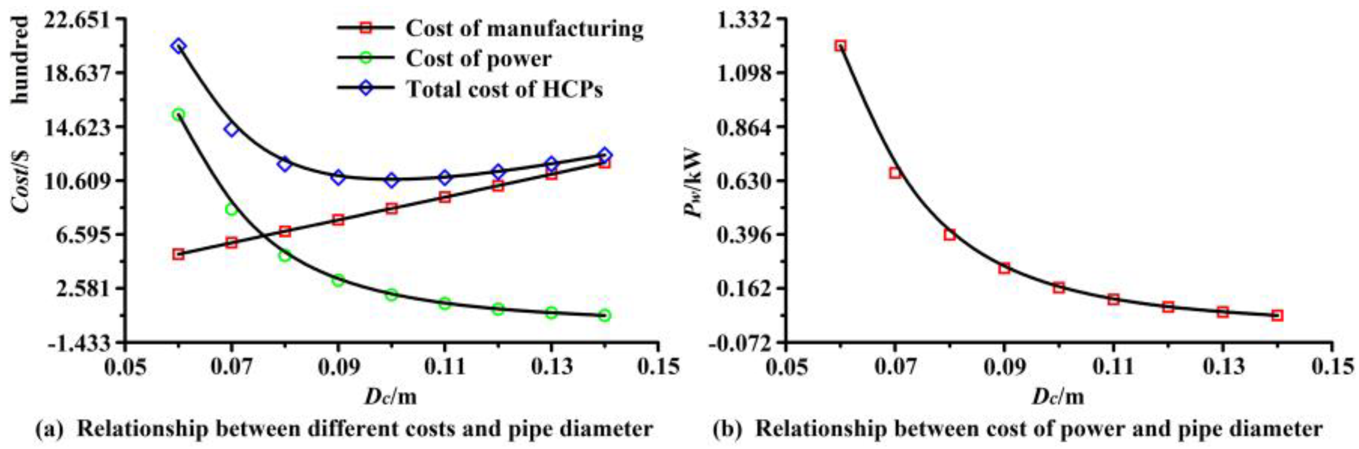
The calculating formula of the piped carriage per unit weight of the piped carriage materials can be expressed as

$$Cos{t}_{Pipedcarriage}={\chi }_2\pi b{D}_c{e}_c{\rho }_{c}g{l}_c+1.5{\chi }_3\pi d_s^2{l}_s{\rho }_{s}g+{\chi }_4{l}_x{m}_x{h}_x{\rho }_{x}g$$

(69)

where χ₂ was the cost coefficient of the barrel per unit weight of the barrel materials; χ₃ was the cost coefficient of the support body per unit weight of the support body materials; χ₄ was the cost coefficient of the sheet-metal plate per unit weight of sheet-metal plate materials; e_c was the thickness of the barrel wall; ρ_c was the density of the barrel; ρ_s was the density of the support bodies; ρ_x was the density of the sheet-metal plate; d_s was the diameter of the support bodies; l_s was the length of the support bodies; l_x, m_x, and h_x were the length, width, and height of the sheet-metal plate, respectively.

7.3. Cost of Power

The cost of power per unit kilowatt hour can be expressed as

$$Cos{t}_{Power}=\frac{{\chi }_5{t}_p{Q}_m\Delta P_{total}}{3.6\times {10}^5{\eta }_p}$$

(70)

where χ₅ was the cost coefficient per unit kilowatt hour; η_p was the efficiency of the centrifugal pumping unit, and generally the efficiency of the industrial centrifugal pumping unit ranged generally between 60% and 75%; t_p was the operating time of the centrifugal pumping unit; P_total was the total pressure drop within the pipelines transporting the piped carriage; Q_m was the mixed pipe discharge. Taking into account the service life of the centrifugal pumping unit, the running time was generally calculated for a one-year period.

HCPs were a typical solid-liquid two-phase flow. To this end, Liu [2] proposed a formula to solve the mixed pipe discharge in Equation (70), which was expressed as

$$Q_m=\frac{\pi D_c^2{U}_{av}}{4}$$

(71)

The above formula only was suitable for a circular pipe. The mixed pipe discharge and pipe discharge in this article were equal in magnitude, but the physical meanings of these two parameters were different. The pipe discharge referred to the fluid mass per hour of single-phase flow at the inlet cross-section of the conveying pipes. The mixed pipe discharge referred to the fluid mass per hour of the two-phase mixing flow of both solid and fluid inside the pipelines.

For the total pressure drop of the carriers transport, the formulas for calculating the total pressure drop within the horizontal pipelines transporting the spherical capsule, the cylindrical capsule and the hexahedral capsule with the density equal to that of its carrier fluid (water) were given in the existing research findings. However, the total pressure drop of the piped carriage transport studied in this article was affected by the transport loading and the rolling frictional resistance for the piped carriage. Therefore, the total pressure drop can only be measured by the numerical simulation of the bidirectional fluid–structure interaction, but not be calculated quantitatively by theories. The studies on the numerical simulation of the bidirectional fluid–structure interaction in Section 4 were of great significance for the establishment of an optimization model of HCPs.

7.4. Optimization Method

The optimization model of HCPs was established to seek the lowest construction cost of the piping system. The construction cost was affected by several factors such as the diameter of the barrel, the length of the barrel, the diameter of the pipeline, the height of the guide vane, the placement angle of the guide vane, the length of the guide vane, and the transport loading. According to the published literature, it can be seen that Model 3 of the piped carriage had the lowest energy losses when transporting along the horizontal pipelines with a diameter of 100 mm. Thus, the optimal diameter ratio of the piped carriage was 0.7 and the optimal length of the barrel was 150 mm. A large number of studies have been conducted on the optimal diameter ratio of piped carriages [57,58]. Combined with the major studies in Section 6, the optimal placement angle of the guide vanes was 21°. Therefore, the model of HCPs can be optimized only by determining the diameter of the conveying pipes.

The solution procedures for determining the diameter of the conveying pipes in the optimization model of HCPs can be expressed as

(1)

Assume the diameter of the pipeline D_c.

(2)

Obtain the total length of the conveying pipe through the dropping and receiving position of the piped carriage L_c.

(3)

Calculate the cost of pipelines and the piped carriage by adopting Equations (68) and (69) based on the materials for the pipelines and the piped carriages and market prices of these materials.

(4)

Determine and configure the physical parameters such as the diameter ratio of the piped carriage, the length of the barrel, the height of the guide vane, the length of the guide vane, the placement angle of the guide vane, as well as the transport loading based on the experimental schemes in Section 2.

(5)

Determine the diameter of the barrel d_c, combined with the diameter of the pipelines.

(6)

Assume the value of the efficiency for the centrifugal pumping unit (0.6–0.75).

(7)

Calculate the total pressure drop of transporting the piped carriage by using the bidirectional fluid–structure interaction method ΔP_total.

(8)

Assume the mixed pipe discharge Q_m, based on the pipe discharge.

(9)

Calculate the cost of power consumption by using Equations (70) and (71) based on the unit price of electricity and the service life of the centrifugal pumping unit.

(10)

Calculate the total cost of HCPs, Cost_Total, using Equations (64) and (65).

(11)

Repeat above Steps 1 to 10 for the various values of the pipe diameters to obtain the minimum value of the total cost of HCPs and its corresponding pipe diameter D_c.

(12)

Find out the optimal diameter of the conveying pipes in order to determine the various indicators for the optimization model of HCPs.

7.5. Design Example

Combined with the contents of Section 6, it was initially found that the energy losses caused by the piped carriage transport within the horizontal pipelines was the lowest when the guide vane placement angle was 21°. Therefore, the piped carriage having the guide vane placement angle of 21° was studied emphatically. The optimization model of HCPs was used to find out the optimal diameter of the conveying pipes and the pumping power required.

Solution: According to the current market, the different constants involved in the optimization model of HCPs can be expressed as

$${\chi }_1=1.575,{\chi }_2=1.837,{\chi }_3=4.724,{\chi }_4=2.435,{\chi }_5=0.139$$

(72)

The billing standard of χ₅ was based on the industrial electricity. In this article, the cost coefficient of the pipelines per unit weight of the pipeline materials χ₁, the cost coefficient of the barrel per unit weight of the barrel materials χ₂, the cost coefficient of the support body per unit weight of the support body materials χ₃, the cost coefficient of the sheet-metal plate per unit weight of sheet-metal plate materials χ₄ and the cost coefficient per unit kilowatt hour χ₅ were defined as the approximate cost coefficients in combination with the actual product costs. From Figure 20a, it can be seen that the cost of manufacturing, the cost of power, and the total costs will be treated as approximate costs. The efficiency of the centrifugal pumping unit was assumed to be 70%. The pipe discharge was 50 m³·h⁻¹ and the transport loading was 0.6 kg. The lengths of both the piped carriage and the conveying pipes were 0.15 m and 28.26 m, respectively. The thicknesses of both the pipe wall and the piped carriage wall were 5 mm and 3 mm, respectively. The rolling frictional resistance coefficient between the piped carriage wall and the Plexiglas pipe wall was 0.428, which was obtained through experiment. The length of the guide vane was 150 mm, its height was 10 mm and its placement angle was 21°. The bidirectional fluid–structure interaction method was used to obtain the total pressure drop of transporting the piped carriage within the horizontal pipelines. From Figure 20a, the optimal diameter of the pipe was 100 mm because the total cost of HCPs was the minimum at D_c = 100 mm, which further validated that it was reasonable to analyze the hydraulic characteristics of transporting the piped carriage with the guide vanes within the pipelines by using the pipe diameter of 100 mm. As shown in Figure 20a, with increase of the pipe diameter, the manufacturing cost of both the pipelines and the piped carriage gradually increased. This variation occurred because the conveying pipes and the piped carriage of larger diameters were more expensive than that of relatively small diameters in terms of the material costs. However, as the pipe diameter increased, the cost of power gradually decreased. The decrease in the cost of power was due to the fact that the decrease in the average axial velocity for a bigger diameter pipe led to a drastic decrease in the energy losses within the pipelines when the pipe discharge was the same. In addition, the total cost of HCPs gradually first decreased from pipeline diameter of 60–100 mm, and then gradually increased with the increase of the pipe diameter. Hence, the optimal pipe diameter corresponding to the minimum cost of HCPs was 100 mm, and the power of the pumping unit corresponding to the optimal pipe diameter was 0.165 kW. Furthermore, based on the optimal pipe diameter, it can be seen that the diameter of the piped carriage in HCPs was set to 70 mm. From Figure 20b, it can be seen that as the diameter ratio increased, the power of the centrifugal pumping unit gradually decreased. The main reason was due to the fact that the variation trends of the pumping unit power and the cost of power consumption were identical, therefore, the pumping unit power gradually decreased with the increase of the pipe diameter.

8. Conclusions

In this article, the structure of the piped carriage was improved by installing the guide vanes on the lateral wall of the barrel, and the hydraulic characteristics of transporting the piped carriage with the different guide vane placement angles within the horizontal pipelines were studied by using the model testing and the numerical simulation. The simulated results were in good agreement with the experimental results, and the maximum relative errors of the hydraulic elements such as the instantaneous axial speed of the piped carriage, the piezometric heads through the pipelines, and the axial velocity distributions of some typical cross-section did not exceed 5.5%, which showed that the bidirectional fluid–structure interaction numerical simulation had obvious advantages for the analysis of HCPs compared with the unidirectional fluid–structure interaction methods. The main conclusions of this study are summarized as follows:

(1)

With the increase of the guide vane placement angle, the average axial speeds of the piped carriage showed a logarithmic growth trend, while the average angular speeds showed an exponential growth trend.

(2)

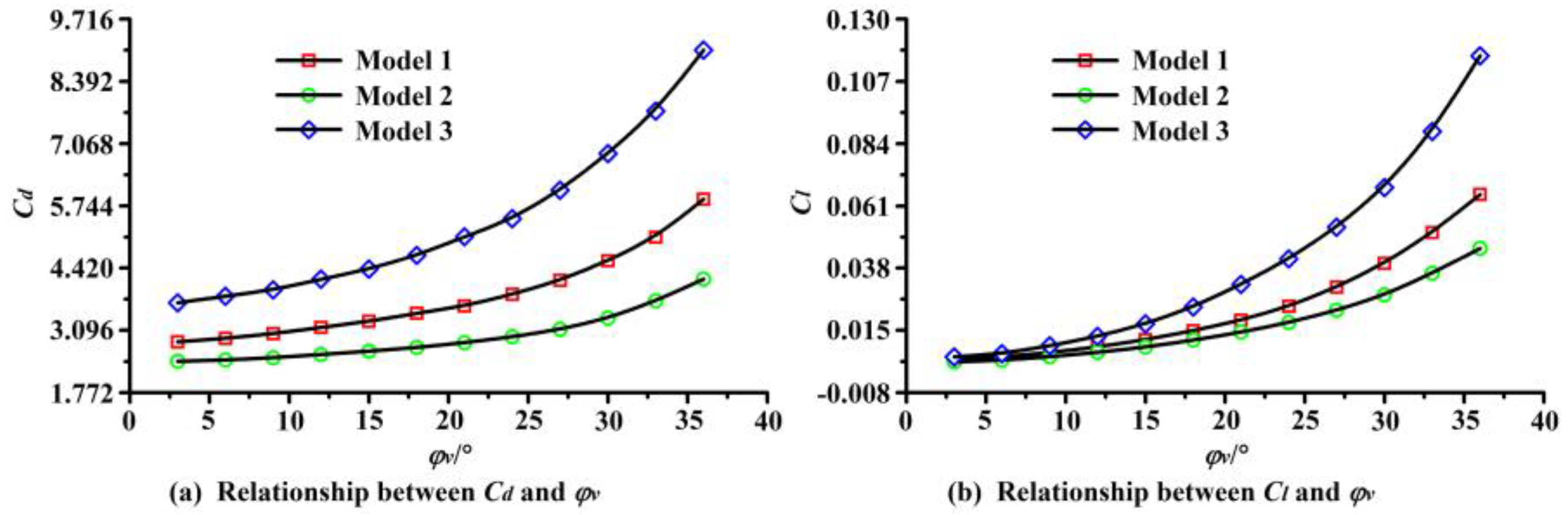
With the increase of the guide vane placement angle, the affected areas of the axial velocity and radial velocity gradually decreased, and the affected areas of the circumferential velocity and vorticity magnitude gradually increased near the front end of the piped carriage. With the increase of the guide vane placement angle, both the average drag coefficient and the average lift coefficient of the piped carriage showed exponential growth.

(3)

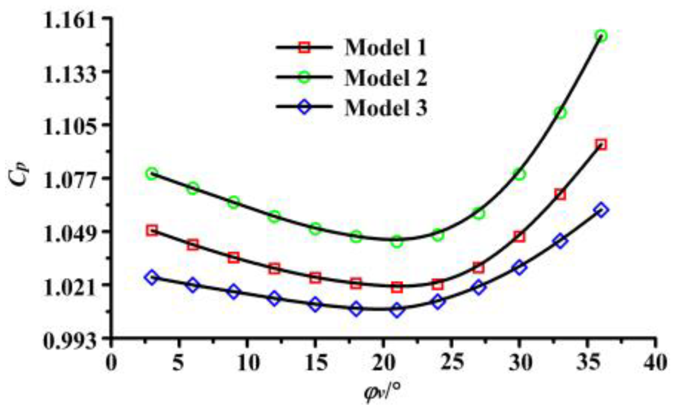
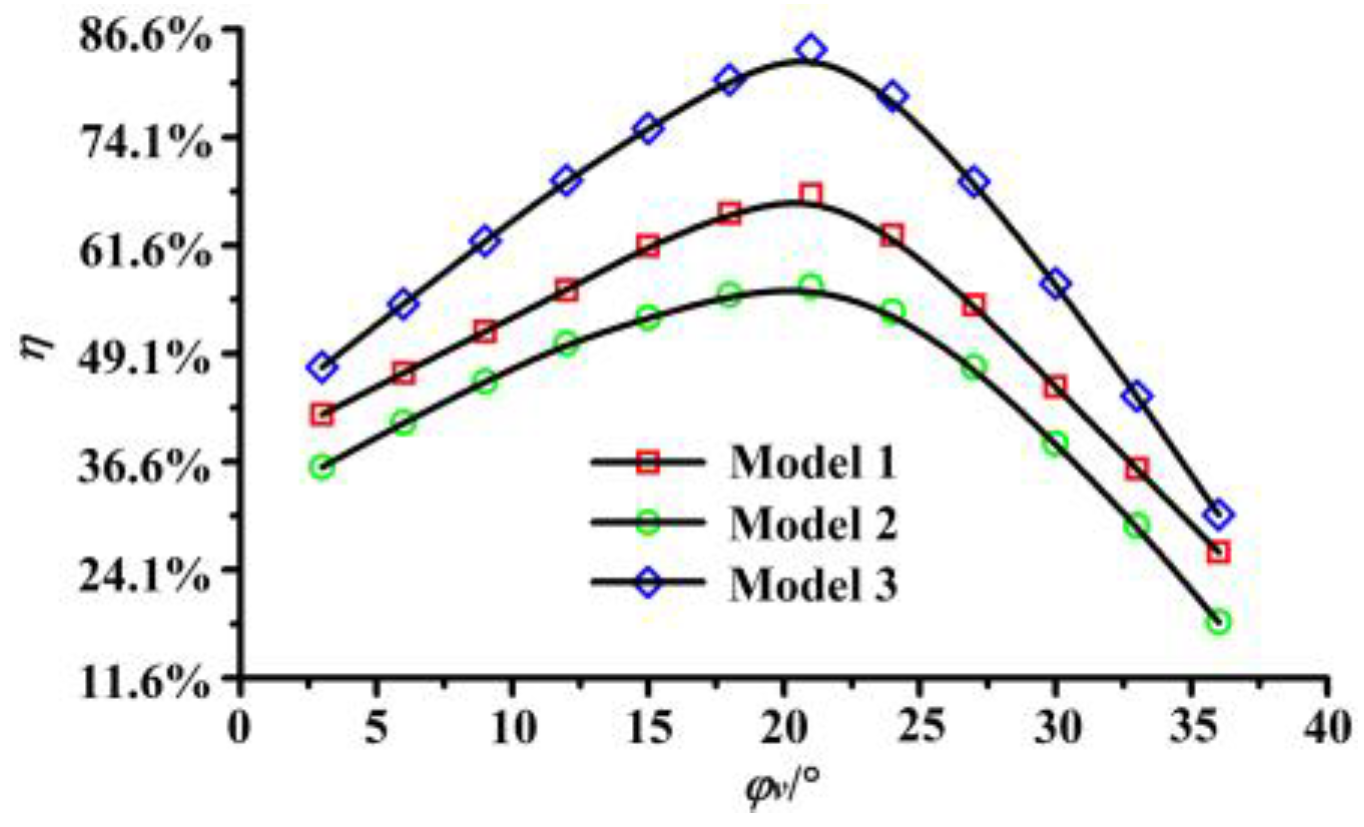
The combined effects of both the energy dissipation and the energy conversion caused the local low-pressure areas to develop near the front end of the piped carriage, and the energy conversion caused the downstream pressure of the piped carriage to rise sharply again. With the increase of the guide vane placement angle, the average pressure drop coefficient of transporting the piped carriage first decreased and then increased, while the mechanical efficiency of transporting the piped carriage first increased and then decreased. The average pressure drop coefficient and mechanical efficiency of the piped carriage collectively indicated that the optimal placement angle of the guide vanes was 21° when the transport loading was 0.6 kg and the pipe discharge was 50 m³·h⁻¹.

(4)

In the near-wall areas of the piped carriage, the axial velocity distributions, radial velocity distributions, circumferential velocity distributions, and vorticity magnitude distributions were basically the same, while the pressure distributions showed a gradually decreasing trend, when the piped carriage moved through the pipelines.

(5)

Based on the least cost principle, the optimization model of HCPs can output the optimal pipe diameter. A practical example has been completed in order to demonstrate the usage and effectiveness of this optimization model.

The research in this article not only provided a practical research method for the technology of hydraulic capsule pipelines, but also offered an abundant theoretical basis for the rational design and extensive application of this technology.

References

1. Tachibana, M.; Matsumoto, Y. Basic studies on hydraulic capsule transportation: Part 1. Loss due to cylindrical capsules set in circular pipe flow. Bull. JSME 1981, 24, 987–994. [Google Scholar] [CrossRef]
2. Liu, H.; Rhee, K.H. Behavior of non-uniform-density capsules in HCP. J. Pipeline 1987, 6, 307–318. [Google Scholar]
3. Brown, R.A.S. Capsule pipeline research at the Alberta Research Council, 1985–1978. J. Pipeline 1987, 6, 75–82. [Google Scholar]
4. Charles, M.E. The pipeline flow of capsules: Part 2: Theoretical analysis of the concentric flow of cylindrical forms. Can. J. Chem. Eng. 1962, 41, 46–51. [Google Scholar]
5. Ellis, H.S. The pipeline flow of capsules: Part 5: An experimental investigation of the transport by water of single spherical capsules with density greater than that of the water. Can. J. Chem. Eng. 1964, 42, 155–161. [Google Scholar] [CrossRef]
6. Round, G.F.; Bolt, L.H. The pipeline flow of capsules: Part 8: An experimental investigation of the transport in oil of single, denser-than-oil, spherical and cylindrical capsules. Can. J. Chem. Eng. 1965, 43, 197–205. [Google Scholar] [CrossRef]
7. Kruyer, J.; Snyder, W.T. Relationship between capsule pulling force and pressure gradient in a pipe. Can. J. Chem. Eng. 1975, 53, 378–383. [Google Scholar] [CrossRef]
8. Latto, B.; Chow, K.W. Hydrodynamic transport of cylindrical capsules in a vertical pipeline. Can. J. Chem. Eng. 1982, 60, 713–722. [Google Scholar] [CrossRef]
9. Tomita, Y.; Yamamoto, M.; Funatsu, K. Motion of a single capsule in a hydraulic pipeline. J. Fluid Mech. 1986, 171, 495–508. [Google Scholar] [CrossRef]
10. Kroonenberg, H.H.V.D. A mathematical model for concentric horizontal capsule transport. Can. J. Chem. Eng. 1987, 56, 538–543. [Google Scholar] [CrossRef]
11. Polderman, H.G.; Velraeds, G.; Knol, W. Turbulent lubrication flow in an annular channel. J. Fluids Eng. 1986, 108, 185–192. [Google Scholar] [CrossRef]
12. Chow, K.W. An Experimental Study of the Hydrodynamic Transport of Spherical and Cylindrical Capsules in a Vertical Pipeline. Master’s Thesis, McMaster University, Hamilton, ON, Canada, 1979. [Google Scholar]
13. Sud, I.; Chaddock, J.B. Drag calculations for vehicles in very long tubes from turbulent flow theory. J. Fluid Eng. 1981, 103, 361–366. [Google Scholar] [CrossRef]
14. Fujiwara, Y.; Tomita, Y.; Satou, H.; Funatsu, K. Characteristic of hydraulic capsule transport. JSME Int. J. 1994, 37, 89–95. [Google Scholar] [CrossRef]
15. Cheng, C.C.; Liu, H. Tilt of stationary capsule in pipe. J. Hydraul. Eng. 1996, 122, 90–96. [Google Scholar] [CrossRef]
16. Lenau, C.W.; El-Bayya, M.M. Unsteady flow in hydraulic capsule pipeline. J. Fluid Eng. 1996, 122, 1168–1173. [Google Scholar] [CrossRef]
17. Huang, X.; Liu, H.; Marrero, T.R. Polymer drag reduction in hydraulic capsule pipeline. AIChE J. 1997, 43, 1117–1121. [Google Scholar] [CrossRef]
18. Agarwal, V.C.; Mishra, R. Optimal design of a multi-stage capsule handling multi-phase pipeline. Int. J. Press. Vessels Pip. 1998, 75, 27–35. [Google Scholar] [CrossRef]
19. Vlasak, P. An experimental investigation of capsules of anomalous shape conveyed by liquid in a pipe. Powder Technol. 1999, 104, 207–213. [Google Scholar] [CrossRef]
20. Yanaida, K.; Tanaka, M. Drag coefficient of a capsule inside a vertical angular pipe. Powder Technol. 1997, 94, 239–243. [Google Scholar] [CrossRef]
21. Azouz, I.; Shirazi, S.A. Numerical simulation of drag reducing turbulent flow in annular conduits. J. Fluid Eng. 1997, 119, 838–846. [Google Scholar] [CrossRef]
22. Sun, X.H.; Li, Y.Y.; Yan, Q.F. Experimental study on starting conditions of the hydraulic transportation on the piped carriage. In Proceedings of the 20th National Conference on Hydrodynamics, Taiyuan, China; 425–431 August 2007. [Google Scholar]
23. Wang, R.; Sun, X.H.; Li, Y.Y. Transportation characteristics of piped carriage with different Reynolds numbers. J. Drain. Irrig. Mach. Eng. 2011, 29, 343–346. [Google Scholar]
24. Li, Y.Y.; Sun, X.H.; Yan, Y.X. Hydraulic characteristics of tube-contained raw material hydraulic transportation under different loads on the piped carriage. Trans. Chin. Soc. Agric. Mach. 2008, 39, 93–96. [Google Scholar]
25. Zhang, X.L.; Sun, X.H.; Li, Y.Y.; Xi, X.N.; Guo, F.; Zheng, L.J. Numerical investigation of the concentric annulus flow around a cylindrical body with contrasted effecting factors. J. Hydrodyn. 2015, 27, 273–285. [Google Scholar] [CrossRef]
26. Wang, J.; Sun, X.H.; Li, Y.Y. Analysis of pressure characteristics of tube-contained raw material pipeline hydraulic transportation under different discharges. In Proceedings of the International Conference on Electrical, Mechanical and Industrial Engineering (ICEMIE), Phuket, Thailand, 24–25 April 2016; pp. 44–46. [Google Scholar]
27. Vlasak, P.; Berman, V. A contribution to hydrotransport of capsules in bend and inclined pipeline sections. Handb. Powder Technol. 2001, 10, 521–529. [Google Scholar]
28. Ulusarslan, D. Comparison of experimental pressure gradient and experimental relationships for the low density spherical capsule train with slurry flow relationships. Powder Technol. 2008, 185, 170–175. [Google Scholar] [CrossRef]
29. Khalil, M.F.; Kassab, S.Z.; Adam, I.G.; Samaha, M.A. Turbulent flow around single concentric long capsule in a pipe. Appl. Math. Model. 2010, 34, 2000–2017. [Google Scholar] [CrossRef]
30. Asim, T.; Mishra, R. Computational fluid dynamics based optimal design of hydraulic capsule pipelines transporting cylindrical capsules. Powder Technol. 2016, 295, 180–201. [Google Scholar] [CrossRef] [Green Version]
31. Asim, T.; Mishra, R.; Abushaala, S.; Jain, A. Development of a design methodology for hydraulic pipelines carrying rectangular capsules. Int. J. Press. Vessels Pip. 2016, 146, 111–128. [Google Scholar] [CrossRef] [Green Version]
32. Li, Y.Y.; Sun, X.H.; Xu, F. Numerical simulation on the piped hydraulic transportation of tube-contained raw material based on FLOW-3D. Syst. Eng.-Theory Pract. 2013, 33, 262–266. [Google Scholar]
33. Feng, J.; Huang, P.Y.; Joseph, D.D. Dynamic simulation of the motion of capsules in pipelines. J. Fluid Mech. 1995, 286, 201–227. [Google Scholar] [CrossRef]
34. Jiang, Q.L.; Zhai, L.L.; Wang, L.Q.; Wu, D.Z. Fluid-structure interaction analysis of annular seals and rotor systems in multi-stage pumps. J. Mech. Sci. Technol. 2013, 27, 1893–1902. [Google Scholar] [CrossRef]
35. Wang, S.B.; Li, S.B.; Song, X.Z. Investigations on static aeroelastic problems of transonic fans based on fluid-structure interaction method. Proc. Inst. Mech. Eng. Part A J. Power Energy 2016, 230, 685–695. [Google Scholar] [CrossRef]
36. Carravetta, A.; Antipodi, L.; Golia, U.; Fecarotta, O. Energy saving in a water supply network by coupling a pump and a pump as turbine (PAT) in a turbopump. Water 2017, 9, 62. [Google Scholar] [CrossRef]
37. Kosugi, S. Effect of traveling resistance factor on pneumatic capsule pipeline system. Powder Technol. 1999, 104, 227–232. [Google Scholar] [CrossRef]
38. Li, Y.Y.; Sun, X.H.; Li, F.; Wang, R. Hydraulic characteristics of transportation of different piped carriages in pipe. J. Drain. Irrig. Mach. Eng. 2010, 28, 174–178. [Google Scholar]
39. Zhang, C.J.; Sun, X.H.; Li, Y.Y.; Zhang, X.Q. Numerical simulation of hydraulic characteristics of cyclical slit flow with moving boundary of tube-contained raw materials pipelines hydraulic transportation. Trans. Chin. Soc. Agric. Eng. 2017, 33, 76–85. [Google Scholar]
40. Teke, I.; Ulusarslan, D. Mathematical expression of pressure gradient in the flow of spherical capsules less dense than water. Int. J. Multiph. Flow 2007, 33, 658–674. [Google Scholar] [CrossRef]
41. Ulusarslan, D.; Teke, I. Comparison of pressure gradient correlations for the spherical capsule train flow. Part. Sci. Technol. 2008, 26, 285–295. [Google Scholar] [CrossRef]
42. Fan, F.; Liang, B.C.; Li, Y.R.; Bai, Y.C.; Zhu, Y.J.; Zhu, Z.X. Numerical investigation of the influence of water jumping on the local scour beneath a pipeline under steady flow. Water 2017, 9, 642. [Google Scholar] [CrossRef]
43. Stancanelli, L.M.; Musumeci, R.E.; Foti, E. Computational fluid dynamics for modeling gravity currents in the presence of oscillatory ambient flow. Water 2018, 10, 635. [Google Scholar] [CrossRef]
44. Vagnoni, E.; Andolfatto, L.; Richard, S.; Münch-Alligné, C.; Avellan, F. Hydraulic performance evaluation of a micro-turbine with counter rotating runners by experimental investigation and numerical simulation. Renew. Energy 2018, 126, 943–953. [Google Scholar] [CrossRef]
45. Zi, D.; Wang, F.J.; Tao, R.; Hou, Y.K. Research for impacts of boundary layer grid scale on flow field simulation results in pumping station. J. Hydraul. Eng. 2016, 47, 139–149. [Google Scholar]
46. Rahimi, H.; Schepers, J.G.; Shen, W.Z.; Ramos García, N.; Schneider, M.S.; Micallef, D.; Simao Ferreira, C.J.; Jost, E.; Klein, L.; Herráez, I. Evaluation of different methods for determining the angle of attack on wind turbine blades with CFD results under axial inflow conditions. Renew. Energy 2018, 125, 866–876. [Google Scholar] [CrossRef] [Green Version]
47. Taghinia, H.; Rahman, M.; Lu, X. Effects of different CFD modeling approaches and simplification of shape on prediction of flow field around manikin. Energy Build. 2018, 170, 47–60. [Google Scholar] [CrossRef]
48. Bambauer, F.; Wirtz, S.; Scherer, V.; Bartusch, H. Transient DEM-CFD simulation of solid and fluid flow in a three dimensional blast furnace model. Powder Technol. 2018, 334, 53–64. [Google Scholar] [CrossRef]
49. Zhang, J.H.; Chao, Q.; Xu, B. Analysis of the cylinder block tilting inertia moment and its effect on the performance of high-speed electro-hydrostatic actuator pumps of aircraft. Chin. J. Aeronaut. 2018, 31, 169–177. [Google Scholar] [CrossRef]
50. Lv, Z.; Huang, C.Z.; Zhu, T.H.; Wang, J.; Hou, R.G. A 3D simulation of the fluid field at the jet impinging zone in ultrasonic-assisted abrasive waterjet polishing. Int. J. Adv. Manuf. Technol. 2016, 87, 3091–3103. [Google Scholar] [CrossRef]
51. Bailoor, S.; Annangi, A.; Seo, J.H.; Bhardwaj, R. Fluid–structure interaction solver for compressible flows with applications to blast loading on thin elastic structures. Appl. Math. Model. 2017, 52, 470–492. [Google Scholar] [CrossRef] [Green Version]
52. Zhu, S.Q.; Hai-Yuan, L.I.; Chen, Z.H.; Huang, Z.G.; Zhang, H.H. Numerical investigations on missile separation of an aircraft based on CFD/CSD two-way coupling method. Eng. Mech. 2017, 34, 217–248. [Google Scholar]
53. Yin, T.Y.; Pei, J.; Yuan, S.Q.; Osman, M.K.; Wang, J.B.; Wang, W.J. Fluid-structure interaction analysis of an impeller for a high-pressure booster pump for seawater desalination. J. Mech. Sci. Technol. 2017, 31, 5485–5491. [Google Scholar] [CrossRef]
54. Zou, D.Y.; Xu, C.G.; Dong, H.B.; Liu, J. A shock-fitting technique for cell-centered finite volume methods on unstructured dynamic meshes. J. Comput. Phys. 2017, 345, 866–882. [Google Scholar] [CrossRef]
55. Asim, T.; Algadi, A.; Mishra, R. Effect of capsule shape on hydrodynamic characteristics and optimal design of hydraulic capsule pipelines. J. Pet. Sci. Eng. 2018, 161, 390–408. [Google Scholar] [CrossRef]
56. Zhu, M.L.; Yang, X.D.; Tian, F.W. The optimal design for long distance conduit of pumping station. J. Hydraul. Eng. 1998, S1, 106–109. [Google Scholar]
57. Shu, D.F. The Research on Hydraulic Characteristics of Migration of Pipe Carriage under Different Diameter Ratios. Master’s Thesis, Taiyuan University of Technology, Taiyuan, China, 2010. [Google Scholar]
58. Sun, L.; Sun, X.H.; Li, Y.Y.; Jing, Y.H. Cyclical slit flow of concentricity under different diameter ratios. Yellow River 2014, 36, 110–113. [Google Scholar]
Figure 1. Entity structure of a piped carriage. Note: 1. Barrel. 2. Support bodies. 3. Universal balls. 4. Guide vanes.
Water 10 01378 g001
Figure 2. Structural diagram of a piped carriage. Note: 1. Pipeline. 2. Barrel. 3. Support bodies. 4. Universal balls. 5. Guide vanes. Dc represents pipe diameter. dc represents diameter of a barrel. lc represents length of a barrel. φv represents placement angle of a guide vane.
Water 10 01378 g002
Figure 3. The force analysis on a piped carriage.
Water 10 01378 g003
Figure 4. Experimental system. Note: 1. Centrifugal pump. 2. Steel penstocks. 3. Surge tank. 4. Regulating valve. 5. Electromagnetic flowmeter. 6. Input port for a piped carriage. 7. Braking device. 8. Rotating control device. 9. Millisecond photoelectric timing devices. 10. Pressure sensors. 11. Piped carriage. 12. Rectangular water channel. 13. Test section. 14. Distributor box. 15. Personal computer. 16. Signal receiver platform of laser Doppler anemometry. 17. Laser Doppler anemometry. 18. High-speed camera. 19. Digital displayer of millisecond photoelectric timing devices. 20. Standard dynamic pressure collection system. 21. 180° pipe bend. 22. Horizontal pipe. 23. Plastic recycling bins. 24. Water temperature control device. 25. Water tank and energy-eliminated orifice plate.
Water 10 01378 g004
Figure 5. Mathematical model. Note: AB represents inlet cross-section of a mathematical model. CD represents outlet cross-section of a mathematical model. AC and BD represent the pipe wall of a mathematical model, respectively. Dc represents pipe diameter.
Water 10 01378 g005
Figure 6. Meshing of computational domains in geometric model.
Water 10 01378 g006
Figure 7. Flow diagram of bidirectional fluid–structure interaction analysis. Note: S represents range of motion for a piped carriage. Si represents instantaneous displacement of a piped carriage at any time.
Water 10 01378 g007
Figure 8. Comparison of simulated results and experimental results for both instantaneous axial speeds and instantaneous angular speeds of a piped carriage. Note: Vaz represents average axial speed of a piped carriage. Vcz represents instantaneous axial speed of a piped carriage. ω represents average angular speed of a piped carriage. ω represents instantaneous angular speed of a piped carriage. φv represents placement angle of a guide vane.
Water 10 01378 g008
Figure 9. Comparison of simulated results and experimental results for piezometric heads through a pipeline. Note: Hp represents piezometric head. φv represents placement angle of a guide vane.
Water 10 01378 g009
Figure 10. Comparison of simulated results and experimental results for axial velocity at horizontal position. Note: Uax represents axial velocity of pipe fluid. φv represents placement angle of a guide vane.
Water 10 01378 g010
Figure 11. Relationship between both average axial speeds and average angular speeds of piped carriages and placement angles of guide vanes. Note: Vaz represents average axial speed of a piped carriage. ω represents average angular speed of a piped carriage. φv represents placement angle of a guide vane.
Water 10 01378 g011
Figure 12. Axial velocity distributions of transporting a piped carriage within a pipeline. Note: φv represents placement angle of guide vane. Scz represents instantaneous displacement of a piped carriage. Vaz represents average axial speed of a piped carriage. Vcz represents instantaneous axial speed of a piped carriage. θ represents instantaneous angle of a piped carriage. ω represents average angular speed of a piped carriage. ω represents instantaneous angular speed of a piped carriage. t represents time. Dc represents pipe diameter.
Water 10 01378 g012
Figure 13. Radial velocity distributions of transporting a piped carriage within a pipeline.
Water 10 01378 g013
Figure 14. Circumferential velocity distributions of transporting a piped carriage within a pipeline.
Water 10 01378 g014
Figure 15. Pressure distributions of transporting a piped carriage within a pipeline.
Water 10 01378 g015
Figure 16. Vorticity magnitude distributions of transporting a piped carriage within a pipeline.
Water 10 01378 g016
Figure 17. Relationship between average pressure drop coefficient and placement angle of guide vanes. Note: Cp represents average pressure drop coefficient of piping system. φv represents placement angle of a guide vane.
Water 10 01378 g017
Figure 18. Relationship between mechanical efficiency and placement angle of guide vanes. Note: η represents the mechanical efficiency. φv represents placement angle of a guide vane.
Water 10 01378 g018
Figure 19. Relationship between force statistics and guide vane placement angle for a piped carriage. Note: Cd represents average drag coefficient of a piped carriage. Cl represents average lift coefficient of a piped carriage. φv represents placement angle of a guide vane.
Water 10 01378 g019
Figure 20. Relationship between different parameters in an optimization model of HCPs and pipe diameter. Note: Cost represents various cost. Pw represents pumping unit power. Dc represents pipe diameter.
Water 10 01378 g020