Valuing the Recreation Benefits of Natural Springs in Florida

Abstract

Karst springs are scenic natural resources in karst areas of Florida, currently under threat from increasing groundwater withdrawal from the Floridan Aquifer and pollution resulting from a variety of sources. This paper estimates the current recreation benefits from visiting springs using the travel cost method and elicits residents’ willingness to contribute for springs restoration using the contingent valuation method. It further compares the performance of count data models correcting for endogenous stratification and truncation, and finds that the annual consumer surplus per person per trip is between $20 and $43, and the annual total recreational value for the four springs studied is about $25 million. Furthermore, visitors are willing to contribute $12 to $14 per person per trip for springs restoration without reducing trip demand.

1. Introduction

Springs, once described as “bowls of liquid light” [1], are one of Florida’s most scenic natural resources. As a result of the karst landform in Florida, these springs are formed when the groundwater from the Floridan Aquifer is under pressure and flows out through a natural opening in the ground [2]. Over 1000 springs have been documented in Florida, representing the highest concentration of springs on Earth [3]. The stable flow rate of spring-run rivers and their relatively constant water temperature make springs ideal habitats for many unique native and migratory species, including the bald eagle, river otter, and West Indian manatee [4]. Additionally, springs are popular destinations for swimming, snorkeling, canoeing, picnicking, and diving [4,5,6]; they are one of the oldest tourist attractions in Florida.

The health and quantity of groundwater in the Floridan Aquifer are critical for the survival of springs and their unique ecosystems. Droughts and overpumping of groundwater to supply population growth and support irrigated agricultural production have been linked to reductions in spring flow [4,7]. Pollution from fertilizers, pesticides, and septic tanks has resulted in elevated nutrient concentrations [4,8]. As a result, native aquatic plants and biodiversity in the springs have declined, and the populations of filamentous algae have increased [4,9]. For example, macroscopic algae are now observed in most springs, and 50% of spring bottoms are covered by macroalgae [9]. Several springs that were once popular swimming holes have diminished to a trickle or have been closed to the public due to poor water quality [4].

The state of Florida provided $191 million for springs restoration between 2012 and 2017 [10]. To prevent further degradation, at least $16 million dollars during the 2017/18 fiscal year was designated for eight projects in the Suwannee River Water Management District (SRWMD) to improve aquifer recharge and septic sewer systems, acquire land, and encourage the adoption of water management practices by agricultural and urban users [10]. Given the volume of tourism and recreation occurring at Florida springs, estimating recreational benefits is a critical step to understanding some of the potential values generated by these kinds of springs restoration projects.

Other cold water springs around the world also provide valuable services to society including providing irrigation and drinking water, supporting biodiversity and habitats, and providing recreation and aesthetic values. Increased water extraction and other economic activities have caused many springs to deteriorate [11]. Understanding the uses and identifying the values provided by springs provide crucial information for effective management, protection, and restoration of springs.

This study contributes to the limited literature focusing on the valuation of springs by estimating the recreational benefits provided by springs in the lower Suwannee and Santa Fe River Basin. This basin includes many iconic springs in spring-fed freshwater river systems that are popular for outdoor recreation yet are experiencing rapid environmental decline. Additionally, we estimate visitors’ willingness to contribute to preserve the springs, thereby providing empirical evidence on the extent to which revenues generated by visitors could be used to support and sustain springs restoration. In contrast, previous studies have documented the economic impact of springs on the local economy [6,8] and a few have examined the recreation benefits of springs in a limited geographic area (i.e., in the Ocala National Forest) or focused on unique recreation activities such as cave-diving [12,13,14]. Furthermore, this study considers the correction for endogenous stratification due to onsite sampling to more precisely estimate the recreation benefits of springs. In contrast, previous studies on springs in Florida using data collected through intercept surveys have not corrected for endogenous stratification. The consumer surplus is likely to be overestimated without correction since onsite data are endogenously stratified by trip frequency and frequent visitors are more likely to be included in the sample.

While many studies use only one valuation method, this survey includes two valuation methods, allowing for a critique of methods. In this study, we demonstrate that contingent valuation methods may result in estimates that are biased downward due to the existence of other related prices that create an arbitrary ceiling on their reported valuation. For our respondents, entrance fees at private springs appear to limit their stated valuation relative to their revealed valuation.

The following sections briefly review related economic literature, summarize data collection and survey responses, present the econometric models of and results from the travel cost and contingent valuation methods, and provide conclusions.

2. Related Economic Literature

Economic studies on the recreation values provided by marine resources, beaches, freshwater rivers, and lakes in Florida have been extensive, but the majority of these studies focus on marine resources (see References [15,16,17] for a review on earlier studies). For example, the value of a beach day in Florida to non-local visitors was $34 in 1984 [15]. The estimated willingness to pay per visit was about $2 to $13.40 in 1998 for freshwater sites, such as lakes [16]. Shrestha et al. [18] found that, on average, visitors would pay $74.18 per visit-day for nature-based recreation in the Apalachicola River region in 2001 using the travel cost method. More recently, Ehrlich el al. [19] used the travel cost method to estimate the value of freshwater-based recreation in the St. Johns River Basin in Florida. On average, households in North and Central Florida were willing to pay $93.63 per trip per household.

However, studies focusing on springs in Florida are limited. A few estimated the economic impact, defined as the number of jobs and the amount of value-added and industry output generated directly and indirectly to the local economy, using the regional input–output model [6,8]. The estimated daily expenditure per group and per person is $215 and $34, respectively, to visit Ichetucknee Springs State Park [6]. Using secondary data on the total number of spring visitors, interviews with local business owners and using regional input–output models, Borisova et al. [8] estimated that the total economic contributions of recreational spending on 20 springs included employment of 1160 jobs and a value added of $52.58 million annually.

Other studies on springs have focused on a few springs in a limited geographical region or focused only on cave diving in the springs. Shrestha et al. [12] estimated visitors’ willingness to pay (WTP) for water-based recreation at four springs in the Ocala National Forest using contingent valuation. Day visitors were willing to pay an average of $4.88, given the current facilities at the spring sites. However, they were willing to pay an additional $8.75 and $11.72 (in 2000) for moderately improved and significantly improved facilities, respectively. While Shrestha et al. [12] provides useful estimates specific to the Ocala National Forest, these springs and corresponding trips to them may have different characteristics than the springs in the Suwannee River Basin, which are part of a much larger spring-fed freshwater river system and are not contained within a national forest. Additionally, while an onsite intercept survey was used in Shrestha et al. [12], correction for the endogenous stratified sample by trip frequency was not applied.

Other studies on springs in Florida focused on diving. Huth and Morgan [13] found that divers were willing to pay between $52 and $83 per cave dive and between $9 and $27 per cavern dive (in 2008) using a contingent valuation method. Morgan and Huth [14] also focused on cave divers and found that the per-person per-trip use value of springs was approximately $155 (in 2009) using the travel cost method. In addition, they presented hypothetical scenarios by either adding a new cave diving system or adding land access to the current diving site and found that consumer surplus was increased by $100 and $50, respectively, by these hypothetical additions. These valuation estimates are likely higher than the valuation of the average springs visitor, who is more likely to engage in lower-cost, less-specialized activities like swimming, picnicking, or canoeing. Additionally, these more common activities have more alternative locations than cave-diving, lessening the potential value of a specific site.

Economic studies on springs in other parts of the United States have been scarce. Mueller et al. [20] found an average willingness to pay $32.60 per household for visiting hot springs in the Grand Canyon using choice experiments. However, values from visiting hot springs in the Grand Canyon are less likely to be applicable to Florida’s freshwater springs.

This study contributes to the existing studies by focusing on springs in two important spring-fed river systems and comparing different empirical strategies in travel cost and contingent valuation. This study also corrects for endogenous stratification as a result of collecting data onsite. The estimated benefits can be used to conduct benefit-cost analysis on ongoing springs restoration initiatives.

3. Data Collection

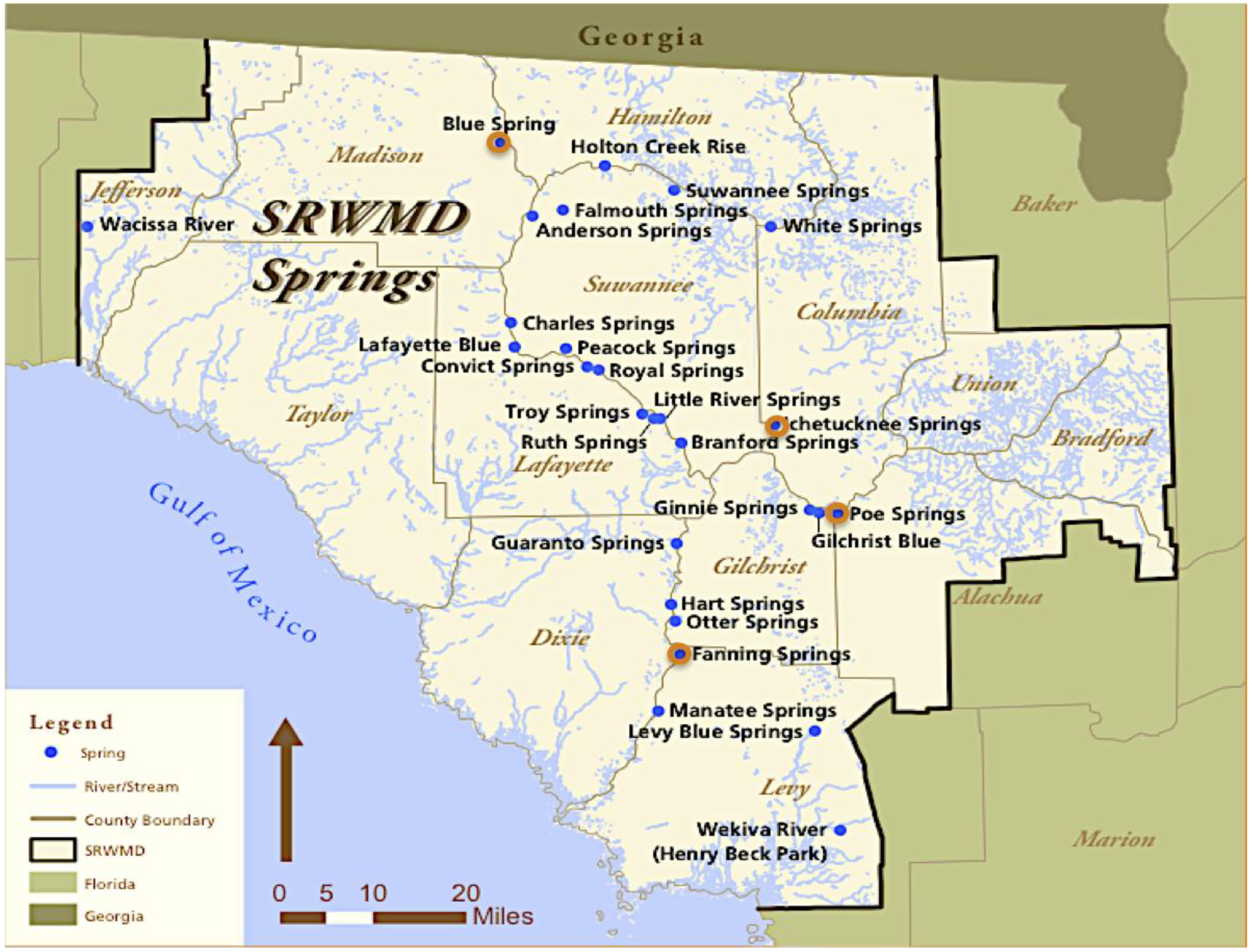
Our research area focused on springs in the Suwannee River and Santa Fe River Basin in North Central Florida, a world-renowned region containing over 300 documented springs. Springs can be classified by discharge. First-magnitude springs discharge more than 2.832 cubic meters per second, and second-magnitude springs discharge between 0.283 and 2.832 cubic meters per second [2]. There are 21 first-magnitude springs in the Suwannee River and Santa Fe River Basin, representing 64% of all the documented first-magnitude springs in the State of Florida. Figure 1 shows the distribution of documented springs in the Suwannee River Water Management District.

We selected four springs in the area since they represent a cross section of springs in the river systems in terms of geographical distribution and outflows. These four springs are highlighted in orange circles in Figure 1. They are frequently visited and offer both water-based and land-based recreation opportunities. Three of them are state parks: Fanning Springs, Ichetucknee Springs, and Blue Springs (Madison County). Another spring named Blue Springs (Gilchrist County) was privately operated and was later purchased by the state of Florida after our survey. Two of the springs, Ichetucknee and Blue Springs (Madison County) are first-magnitude springs; the rest of them are second-magnitude springs.

Table 1. Springs information.

Springs Park	Admission Fee	Main Activities
Blue Springs State Park (Madison)	$2.00–$5.00	Scuba diving, swimming, and picnicking
Ichetucknee Springs State Park	$2.00–$6.00	Tubing, scuba diving (Blue Hole), picnicking, snorkeling, canoeing, swimming, hiking, and wildlife viewing.
Fanning Springs State Park	$2.00–$6.00	Boating, kayaking, swimming, and wildlife viewing
Blue Springs Park (Gilchrist) (private)	$10	Swimming, snorkeling, and underwater photography

summarizes the conditions and recreation opportunities at the four springs.

This study used an onsite intercept survey, which is more cost-effective at targeting visitors. We randomly sampled 494 visitors at these four springs from May 2016 to August 2016 during the peak season for spring visitors in the region. To ensure representativeness of the visitor population, three weekdays and four weekends were randomly selected for the survey in a given month, and equal numbers of respondents were collected among the four springs. All survey participants provided informed consent, and the survey protocol was approved by the University of Florida Internal Review Board (IRB # IRB201600752).

The survey instrument included questions about the respondent’s frequency of trips to the spring in the past year, recreation experiences, and perceptions about water clarity and condition of the facility and green space. It also elicited information on demographics on each of the respondents, such as home zip code, age, education, and household income. Additionally, respondents were presented with a hypothetical increase in entrance fee per person for spring restoration. Respondents were randomly assigned into one of four levels of increases in entrance fees per person: $10, $15, $20, and $25, respectively. Respondents were then asked how their recreation visits to the spring would change based on a Likert scale, including “visit fewer times, about the same, more times, and not sure”. The increase in entrance fee was used as a payment vehicle since the current entrance fee is a small fraction of the total travel cost compared to other tourist attractions in Florida and recreation is the most wide-spread use of springs. For example, the entrance fee to most of the state-operated spring parks was $2 per pedestrian or $4–$6 per vehicle (smaller springs were usually free). In contrast, privately-operated springs charged between $10 and $15 per person. An increase in the entrance fee might be a potential way to generate spring restoration funding.

4. Methods

The travel cost method (TCM) is one of the commonly used revealed preference methods in recreational demand analysis. TCM applies the basis of demand theory to recreational demand in that the travel cost to visit a site represents the price paid for recreation at the site. Individuals who live farther away from the targeted sites pay higher travel costs and thus take fewer trips than those who live closer, based on the basic law of demand. An individual’s valuation of the recreational benefits provided by the natural resource can be revealed by estimating the number of trips taken at a given travel cost. Since the income effect on recreation is typically low and recreation only accounts for a small share of the household budget, the willingness to pay to access the recreation site can be approximated by calculating the consumer surplus, an integral above the travel cost and below the demand curve, based on the estimates of the income-constant recreational demand curve [21].

Given that recreational trip frequency is a nonnegative integer and reported frequencies tend to be small, positive integers, count data models are often used to estimate the recreational demand in the single-site TCM. Suppose the population distribution of trip frequency follows a Poisson process, the probability of observing $y_i$ number of trips for respondent $i$ is shown in Equation (1):

$$Pr\left(Y=y_i\right)=\frac{e^{-{\mu }_i}{u}_i^{y_i}}{y_i!},y=0,1,2,3,\dots$$

(1)

where ${\mu }_i$ indicates the conditional expected value of $y_i$.

Recreational demand observed at the individual level may be influenced by other factors in addition to travel cost. These factors include the household’s income, the presence of a substitute recreation site, quality of the recreation site, and other demographic characteristics, as shown in Equation (2):

$$ln\left(y_i\right)={\beta }_o+{\beta }_{tc}\ast t{c}_i+Z_i^{\prime }{\beta }_1+S_i^{\prime }{\beta }_2+{\epsilon }_i$$

(2)

where $t{c}_i$ represents respondent $i\prime \mathrm{s}$ travel cost to visit the spring, $Z_i$ represents a vector of respondent characteristics, and $S_i$ indicates a vector of spring characteristics and respondent $i\prime \mathrm{s}$ access to a substitute recreation site. The exponential of ε is assumed to follow a gamma distribution. The parameters in Equation (2) can be estimated using maximum likelihood [22].

The consumer surplus per visit can be estimated using −1/${\widehat{\beta }}_{tc}$, where ${\widehat{\beta }}_{tc }$ represents the estimated coefficient for the travel cost variable [21]. Specifically, the consumer surplus represents the access value for the site for an “average” visitor in the underlying visitor population [23]. The total consumer surplus for the entire recreation season is give by Equation (3):

$$C{S}_i=-\frac{{\tilde{u}}_i}{{\widehat{\beta }}_{tc}}$$

(3)

where ${\tilde{u}}_i$ is the expected number of trips to the spring. For its confidence interval, a parametric bootstrapping procedure by Krinsky and Robb [24] can be used to produce the simulated distribution of per group per trip consumer surplus based on 1000 draws from its posterior distribution.

Estimating Equation (2) requires one to take into account the nature of the data collection through the onsite intercept survey. Specifically, trip frequency collected through an onsite survey is a non-negative integer and truncated at 1. Additionally, individuals who take more frequent trips are more likely to be included in the onsite example. In other words, the composition of the sample is endogenously stratified by trip frequency [25].

Shaw showed that correcting for truncation and endogenous stratification by $y$ can be achieved by adjusting the conditional density function of Equation (1) into Equation (4):

$$Pr\left(Y=y_i|Y>0\right)=\frac{e^{-{\mu }_i}{\mu }^{y_i-1}}{\left(y_i-1\right)!}$$

(4)

where $E(y_i|x_i)={\mu }_i+1$ and $Var(y_i|x_i)={\mu }_i$.

However, the Poisson model is restrictive by assuming that the conditional mean and variance are equal. This strong assumption will potentially cause misspecification for many recreational demand data in the presence of overdispersion [26]. A negative binomial model is often used in the presence of overdisperson, and an additional overdispersion parameter is introduced. The Poisson model is a special case of the negative binomial model when the parameter of overdispersion equals zero.

In the presence of truncation only, the conditional density of the truncated negative binomial distribution is shown as Equation (5):

$$r\left(Y=y|Y>0\right)=\frac{\Gamma \left({\alpha }^{-1}+y\right)}{\Gamma \left({\alpha }^{-1}\right)\Gamma \left(y+1\right)}{\left(1+\alpha \mu \right)}^{-(y+{\alpha }^{-1})}{\left(\alpha \mu \right)}^y\left(\frac{1}{1-{\left(1+\alpha \mu \right)}^{-{\alpha }^{-1}}}\right)$$

(5)

where Γ(.) represents the gamma distribution and the parameter α determines the degree of overdispersion.

Englin and Shonkwiler [27] extended Shaw’s [25] correction for the Poisson model to the negative binomial model, as shown in Equation (6):

$$Pr\left(Y=y_i|Y\rangle 0\right)=y_i\frac{\Gamma \left({\alpha }_i{}^{-1}+y_i\right)}{\Gamma \left({\alpha }_i{}^{-1}\right)\Gamma \left(y_i+1\right)}{\left(1+{\alpha }_i{\mu }_i\right)}^{-(y_i+{\alpha }_i{}^{-1})}\frac{{\left({\alpha }_i{\mu }_i\right)}^{y_i}}{{\mu }_i}$$

(6)

where $(y_i|x_i)={\mu }_i+1+{\alpha }_i{\mu }_i$, and $Var(y_i|x_i)={\mu }_i\left(1+{\alpha }_i+{\alpha }_i{\mu }_{i }+{\alpha }_i{}^2{\mu }_i\right)$.

There are several options to parameterize ${\alpha }_i$ [28]. Englin and Shonkwiler [26] chose ${\alpha }_i=\alpha /{\mu }_i$ in their specification, such that

$$Pr\left(Y=y_i|Y\rangle 0\right)=y_i\frac{\Gamma \left({\alpha }^{-1}{\mu }_i+y_i\right)}{\Gamma \left({\alpha }^{-1}{\mu }_i\right)\Gamma \left(y_i+1\right)}{\left(1+\alpha \right)}^{-\left(y_i+{\alpha }^{-1}{\mu }_i\right)}\frac{{\left(\alpha {\mu }_i\right)}^{y_i}}{{\mu }_i}$$

(7)

where $E(y_i|x_i)={\mu }_i+1+\alpha$ and $Var(y_i|x_i)={\mu }_i+\alpha +\alpha {\mu }_{i }+{\alpha }^2$.

Alternatively, Martinez-Espiñeira and Amoako-Tuffour [29] parameterize the dispersion parameter ($a_i)$ by regressing it on selected demographic characteristics of the visitors. Landry et al. [30] parameterized ${\alpha }_i$ with $\alpha {\mu }_i{}^{p-2}$, by introducing an additional parameter $p.$ If $p=1$, it matches Englin and Shonkwiler’s setting of the dispersion parameter. If $p=2$, it becomes negative binomial model with a constant dispersion parameter $a_i=\alpha$ for all respondents.

The selection on the appropriate distribution is based on the information-based criteria and log likelihood values. A likelihood-ratio test can be used to test the significance of the overdispersion parameter for selecting negative binomial versus Poisson model [29]. In this paper, we compare the estimates from standard Poisson model (Poisson), truncated Poisson (TP), and truncated Poisson with endogenous stratification (TPS) by Shaw [24], and the estimates from the negative binomial models (NB), truncated NB (TNB), and truncated NB with endogenous stratification by Englin and Shonkwiler [27] and Martínez-Espiñeira and Amoako-Tuffour [29]. Because having an additional parameter complicates the maximum likelihood estimation and we could not obtain convergence using Landry et al. [30], we use the Akaike information criterion (AIC), Bayesian information criterion (BIC), and the log likelihood values to select the best fit from these models.

To empirically estimate the TCM model, each individual respondent’s travel cost of visiting the study area was estimated using the monetary cost of travel and the opportunity cost of travel time. Following existing studies, we determined the centroid of the visitor’s home zip code to estimate the distance traveled to the recreation location using the Google maps functions in R (http://journal.r-project.org/archive/2013-1/kahle-wickham.pdf). We also elicited information on alternative recreation locations. Most respondents indicated that their alternative choice was within the same river system, and some identified alternative springs, though others were not sure about the exact location of the access point. To avoid bias created by assuming the alternative location to be the nearest point of the river to a visitor’s home as shown in Reference [31], we used a dummy variable to indicate that the respondent had an alternative recreation location. The cost per mile was $0.55 based on the standard mileage rate determined by the Internal Revenue Service of U.S. in 2016, and the average travel speed was assumed to be 40 miles (64 km) per hour. The cost per mile was multiplied with the round-trip travel distance from the centroid of the respondent’s home zip code to the spring to determine the monetary cost of the travel. The opportunity cost of the travel time was calculated by multiplying a fraction of the implicit hourly wage rate by the time spent traveling. Following the TCM literature, the implicit hourly wage rate was calculated as the household income divided by 2080 h, assuming a 40-h workweek for 52 weeks a year. The fraction of this implicit wage rate was assumed to be one third, which is commonly used by existing studies (e.g., References [29,30,31,32,33]).

In addition to estimating the TCM, we analyze the visitors’ responses to the hypothetical increase in entrance fees for a proposed springs restoration program following the contingent valuation method, which is a widely used method to elicit values for proposed policy interventions, such as in Aslam et al. [34] and Kwak et al. [35]. For simplicity and ease of administration during an onsite intercept survey, a single-bounded CV question was used. During the survey, respondents were randomized into four levels of hypothetical increases in entrance fees per person, and were asked if such an increase would affect their future trip demand by reducing their visit frequency, maintaining their visit frequency, or even increasing their trip frequency. We treat their responses as a dichotomous choice variable where maintaining or increasing visit frequency was “yes” in terms of willingness to pay the new entrance fee and reducing trip frequency was “no”.

Following the single-bounded CV model, the probability that a respondent would respond “yes” to a hypothetical increase in entrance fee can be expressed in a basic exponential logistic form parameterized by $\gamma$, as shown in Equation (8):

$${\pi }_{i,\gamma }\left(X_i\right)=\frac{exp\left(X_i{}^{\prime }\gamma \right)}{1+exp\left(X_i{}^{\prime }\gamma \right)}$$

(8)

where ${\pi }_{i,\gamma }\left(X_i\right)$ represents the probability of accepting the increased entrance fee for individual $i$. When there are no other control variables, $X\prime \gamma ={\gamma }_0+{\gamma }_{bid}\ast Fee+v_i,$ where $v_i$ represents the error term. Hanemann [36] and Duffield and Patterson [37] showed that the mean WTP can be approximated using $WTP=\frac{-1}{\widehat{{\gamma }_{bid}}}ln\left(1+exp\left(\widehat{{\gamma }_0}\right)\right).$ When there are control variables represented by a vector of $G,$ we have $X_i^{\prime }\gamma ={\gamma }_0+{\gamma }_{bid}\ast Fee+G^{\prime }{\gamma }_1+v_i$, and the mean WTP is approximated by $WTP=\frac{-1}{\widehat{{\gamma }_{bid}}}ln\left(1+exp\left(\widehat{{\gamma }_0}+\overline{G^{\prime }}\widehat{{\gamma }_1}\right)\right),$ where $\overline{G}$ represents the control variables evaluated at their means [38]. A parametric bootstrapping procedure by Krinsky and Robb [24] can be applied to derive the confidence intervals. The control variables are typically correlated with trip frequency, such as recreation experience and household income.

The estimation of Equation (8) may also suffer from endogenous stratification if avid visitors are more likely to be included in the sample, and their willingness to contribute may be correlated with trip frequency. A few studies, such as Gonzalez et al. [39], discussed the implications of onsite sampling on the estimates using CV. One option is to use auxillary information collected from an offsite survey. González-Sepúlveda and Loomis [40] used exogenous sampling maximum likelihood (WESML) based on Manski and Lerman [41] to correct the parameter estimates on the onsite conditional WTP. The likelihood function is given by:

$$ln L={\displaystyle \sum }_{i=1}^N{w}_i \{d_{i}ln {\pi }_{i,\gamma }\left(X_{2i}\right)+\left(1-d_i\right)ln(1-{\pi }_{i,\gamma }\left(X_{2i}\right)\}$$

(9)

where $w_i=d_i(\frac{p_1}{s_1})+\left(1-d_i\right)(\frac{1-p_1}{1-s_1})$, $p_1$ is the proportion of local visitors to springs among Florida population; $d_i$ is the dummy response variable, where $d_i$ = 1 if the respondent was willing to travel to the site at least as much as before given the increase in entrance fee, and $d_i$ = 0 otherwise; $s_1$ is the observed proportion of respondents in the sample with $d_i$ = 1. However, the key limitation of WESML is that auxiliary information on $p_1$ is required.

In this study, we compared the estimates and the derived mean WTP with control variables and without control variables, and with and without corrections of endogenous stratification in the CV models.

5. Results

The sample includes 494 observations. Respondents’ characteristics were consistent with the Florida census, except for respondents’ household income and educational attainment. Similar to Florida’s population, we found that 55% of the respondents were female, the average age of the respondents was 41 years old, the average household size was 2.2, and 59% of the respondents had full-time jobs. In contrast, the median household income of the respondents is $60,000, which was higher than the median household income of $48,900 in Florida. Our sample had a higher percentage of college-educated respondents at 38.7% with a bachelor’s degree or higher compared to 27.9% of the Florida population.

The majority of the respondents (90%) visited the springs for the sole purpose of recreation; 72% visited the springs during the weekend; 83% took day trips to the springs; and 17% stayed overnight, averaging 3.2 nights at camping sites. The primary recreation activities included swimming (45%), tubing (19%), and picnicking (17%). The other mentioned categories were nature viewing (6%), hiking (5%), kayaking (4%), and camping (2%). Total expenditure reported when visiting the springs was $117.44 per group. The average one-way travel distance was 162 km.

The final dataset used to estimate econometric models included 408 usable observations, focusing on visitors whose primary purpose was for recreation and those who took day trips [41,42]. In addition, those with highly frequent visits (above the 95th percentile) were dropped to decrease the influences of extreme values.

Household income was collected as a categorical response. Following previous studies, we used the mid-points of the categorical responses as the level of household income. However, 18.2% of the respondents declined to reveal their household income during the intercept survey. We ran a linear regression to predict those missing values using the respondent’s education, age, and employment-status, as in Bin et al. [26].

Table 2. Summary statistics for variables.

Variable	Mean	Std. Dev.	Definition
Trip	2.36	3.16	Number of visits to the spring in the past 12 months
Household income	57761	25154	Mid-point of household income brackets ($thousands)
Travel cost	147.11	134.65	Round-trip travel cost
Substitute	0.79	0.41	Dummy variable: 1 if the respondent has identified an alternative site; 0 otherwise
Male	0.45	0.5	Dummy variable: 1 if male; 0 otherwise
Private	0.27	0.44	Dummy variable: 1 if the spring is privately operated; 0 otherwise
Perception for facility	4.00	1.33	Perception for conditions of the facilities at the spring (a 5-point Likert scale, where 1 was “below average” and 5 was “above average”)
Perception for water clarity	4.58	0.90	Perception for water clarity in the spring (a 5-point Likert scale, where 1 was “below average” and 5 was “above average”)
Past experience	0.36	0.48	Dummy variable: 0 if it was the first time to visit the springs; 1 otherwise.

shows the descriptive statistics of variables used in the econometric analysis. The mean number of trips, total travel cost, and household income were 2.36, $147.11, and $57,761, respectively. Most of the respondents (i.e., 79%) indicated that they had alternatives for similar recreation activities if the spring they visited was closed. We asked the respondents to describe their perceptions on the water clarity (cleanliness) of the water in the springs and the conditions of facilities at the spring, using a scale from 1 to 5, where 1 was “below average” and 5 was “above average”. We found that the average perceived water clarity rating was 4.58 and the average rating for the conditions of the facilities was 4.

5.1. Model Estimates

The estimation results of recreation demand are shown in

Table 3. Estimated results of the travel cost models.

	Poisson			Negative Binomial
	Poisson	TP	TPS	NB	TNB	TNBS	GTNBS
Travel cost	−0.32 ***	−0.76 ***	−0.90 ***	−0.28 ***	−0.92 ***	−0.86 ***	−0.86 ***
	(0.05)	(0.13)	(0.16)	(0.04)	(0.20)	(0.10)	(0.10)
Household income	0.01	0.02	0.02	0.00	0.02	0.02	0.02
	(0.03)	(0.03)	(0.04)	(0.02)	(0.05)	(0.03)	(0.03)
Substitute	0.26	0.40	0.48	0.26*	0.49	0.43 **	0.39 *
	(0.16)	(0.36)	(0.42)	(0.15)	(0.44)	(0.22)	(0.22)
Male	−0.08	−0.11	−0.14	−0.07	−0.02	−0.09	−0.76
	(0.12)	(0.17)	(0.21)	(0.11)	(0.25)	(0.15)	(357.22)
Perception for water clarity	0.10	0.19	0.22	0.09	0.27 *	0.22 **	0.21 **
	(0.06)	(0.13)	(0.15)	(0.06)	(0.16)	(0.10)	(0.10)
Perception for facility	0.07	0.09	0.11	0.07*	0.25 **	0.18 ***	0.19 ***
	(0.04)	(0.07)	(0.08)	(0.04)	(0.12)	(0.06)	(0.06)
Private	0.05	0.05	0.06	0.05	0.12	0.07	0.09
	(0.13)	(0.18)	(0.22)	(0.13)	(0.29)	(0.16)	(0.16)
Constant	0.31	−0.20	−0.79	0.30	−18.97 ***	−13.05 *	−16.06
	(0.33)	(0.67)	(0.79)	(0.30)	(1.63)	(6.61)	(219.38)
$ln\left(\alpha \right)$				−0.89 ***	18.34 ***
AIC	1818.20	1600.94	1757.47	1579.80	1123.58	1183.51	1188.51
BIC	1850.29	1633.03	1789.56	1615.90	1159.69	1219.61	1236.65
Log likelihood	−901.10	−792.47	−870.74	−780.90	−552.79	−582.76	−582.26
Observations	408	408	408	408	408	408	408

Standard errors in parentheses: *** p < 0.01, ** p < 0.05, * p < 0.1.

. The first three columns report the estimates from the standard Poisson model (Poisson), truncated Poisson (TP), and truncated Poisson with endogenous stratification (TPS) by Shaw [25], respectively. The remaining columns of

Table 4. Consumer surplus (CS) estimation.

Model	CS/Group per Trip	Expected Number of Trips a	CS/Group per Year	CS/Person per Trip b
NB	$357.14 ($287.89, $471.30)	2.35	$839.29	$94.98
TNB	$108.70 ($76.71, $162.05)	2.33	$253.26	$28.91
TNBS	$116.28 ($95.28, $148.47)	2.35	$273.26	$30.93
GTNBS	$116.28 ($94.74, $149.63)	2.36	$274.42	$30.93
Poisson	$312.50 ($240.18, $444.71)	2.36	$737.50	$83.11
TP	$131.58 ($101.11, $199.58)	2.36	$310.53	$34.99
TPS	$111.11 ($83.48, $166.28)	2.36	$262.22	$29.55

95% confidence intervals are in parentheses. ^a $E(y|x)=\mu$ for models without any correction; $E(y|x)=\frac{u}{1-e^{-\mu }}$ for TP; $E(y|x)=\frac{\mu }{1-{\left(1+\alpha \mu \right)}^{-{\alpha }^{-1}}}$ for TNB; $E(y_i|x_i)={\mu }_i+1$ for TPS; $E(y_i|x_i)={\mu }_i+1+{\alpha }_i{\mu }_i$ for TNBS and GTNBS. ^b Based on an average size of 3.76 per group.

report the estimates from the negative binomial models (NB), truncated NB (TNB), and truncated NB with endogenous stratification (TNBS by Englin and Shonkwiler [27], and GTNBS by Martínez-Espiñeira and Amoako-Tuffour [28]). The overdispersion parameter ($\alpha$) in GNBS was parameterized using the age of the respondent, gender, and the number of adults in a household. First, we performed the likelihood ratio test on the significance of the over dispersion parameter, $\alpha$ = 0, between each of the three pairs (NB and Poisson, TNB and TP, TNBS and TPS) with one degree of freedom. The chi-squared values for these three comparisons were 240.4, 479.36, and 575.96, respectively. They exceeded the critical value, 3.84 for 95% confidence, indicating the presence of overdispersion in the data. The likelihood-ratio tests suggested that all Poisson models were overly restrictive.

Second, among the three sets of estimates based on negative binomial models, the truncated negative binomial (TNB), which accounted only for truncation, provided the best fit, based on the minimized AIC or BIC. This was different from Martinez-Espiñeira and Amoako-Tuffour [29] and Landry et al. [30] who showed models correcting for endogenous stratification and truncation outperform other models that simply corrected for truncation alone. This may be due to the nature of this dataset. The proportion of respondents reported taking only one trip was 61.8% and the percentage reporting two trips was 13.5% of the sample. Only a small fraction of the sample visited the springs more frequently; thus, endogenous stratification by trip frequency was less likely to influence our estimates.

Third, focusing on the results from the truncated negative binomial model (TNB), we found that the coefficient for the travel cost variable was negative (−0.92) and statistically significant, implying a downward-sloping demand curve. A visitor with higher travel costs tended to make fewer visitations, ceteris paribus. Additionally, the estimated coefficients for travel costs were consistent across various negative binomial specifications correcting for truncation and endogenous stratifications. However, without correcting for truncation, standard Poisson and negative binomial estimates were significantly overestimating the coefficients of the travel cost variable.

Finally, the coefficient of household income was insignificant, which was consistent with many studies using TCM [22,40,42]. The coefficients for variables indicating the presence of a substitute recreation site, private ownership of the spring, and the respondent’s gender were also not statistically significant. We found a positive association between trip frequency and respondents’ perception of water clarity and conditions of the facilities. For example, a one unit increase in the Likert scale of the conditions of the facilities was associated with 25% more visits, and a one unit increase in the Likert scale of the perceived water clarity was associated with 27% more visits, holding other variables constant. As expected, better water clarity and better facilities attract more visits.

As a robustness check, we also estimated the TCM as an incomplete demand system in which the availability of an alternative site was excluded in the TCM since the incomplete demand system had to satisfy homogenous degree zero in all prices and income, a requirement for correct welfare analysis as discussed in Reference [43]. The empirical results were qualitatively similar.

5.2. Consumer Surplus

Table 4 reports the estimated consumer surplus from the six TCM estimates. First, without correcting for truncation and endogenous stratification, the consumer surplus estimates from either Poisson or negative binomial models were much larger. This was consistent with other studies that show that consumer surplus was overestimated without correcting for truncation and endogenous stratification [30]. Based on our preferred TCM from the truncated negative binomial estimates, the consumer surplus per visitor-group per trip under TNB was $108.70 with a 95% confidence interval between $76.71 and $162.05.

Dividing the consumer surplus per group by the sample mean of visitor group size, we obtained the consumer surplus per person per trip, which was $28.91 with a 95% confidence interval between $20.40 and $43.10. Compared to other studies on recreation in springs, per person per trip consumer surplus from this paper was higher than the estimates in Shrestha et al. [12] and smaller than Morgan and Huth [14]. Given the average expected trip frequency of 2.33, the annual consumer surplus per person per year is $67.36. Annual consumer surplus can be multiplied by the population of spring visitors in Florida to calculate total annual benefits.

In the absence of the size of the entire visitor population, we could calculate the total consumer surplus for each spring by multiplying the number of annual visitors recorded by the Florida Parks and Recreation with the CS per person per trip. The total recreational value for these four springs was about $25 million annually as shown in

Table 5. Total consumer surplus (CS).

Springs	Annual Day-Trip Visitors (June 2015–June 2016)	Total CS per Year ($)
Blue Springs (Gilchrist)	77,500	2,240,525
Fanning Springs	218,963	6,330,220
Ichetucknee Springs	507,238	14,664,251
Blue Springs (Madison)	48,209	1,393,722
Overall	851,910	24,628,718

. Ichetucknee Springs was the most popular spring and thus had the highest annual use value. The formerly privately-operated Blue Springs was valued at $2.24 million.

5.3. Willingness to Contribute

Table 6. Coefficient estimates of contingent valuation models.

	Without Controls		With Controls
	(1)	(2)	(3)	(4)
	Uncorrected	Corrected	Uncorrected	Corrected
Bid value	−0.104 ***	−0.105 ***	−0.109 ***	−0.110 ***
	(0.022)	(0.022)	(0.022)	(0.022)
Household income			0.094 **	0.093 **
			(0.047)	(0.047)
Travel distance to the spring			0.367 **	0.362 **
			(0.147)	(0.145)
Male			0.087	0.085
			(0.229)	(0.229)
Perception for water clarity			0.064	0.063
			(0.123)	(0.123)
Perception for facility			0.018	0.020
			(0.089)	(0.088)
Past experience			−0.077	−0.081
			(0.261)	(0.261)
Constant	1.199 ***	1.007 ***	−1.230	−1.399
	(0.385)	(0.384)	(1.007)	(1.005)
AIC	480.437	427.710	475.819	425.377
BIC	488.385	435.658	507.610	457.167
Log likelihood	−238.219	−211.855	−229.910	−204.688
Observations	393	393	393	393
Mean WTP	$14.06 ($11.15, $21.51)	$12.57 ($10.06, $18.92)	$13.73 ($11.03, $20.75)	$12.26 ($9.98, $18.37)

Standard errors in parentheses: *** p < 0.01, ** p < 0.05, * p < 0.1.

shows the results for CV models. Columns 1 and 3 report the estimated logit models without correcting for endogenous stratification, and Columns 2 and 4 report the corrected estimates. Estimates in Columns 1 and 2 only include the randomized hypothetical increase in the entrance fee, and Columns 3 and 4 include other control variables.

To correct for endogenous stratification with WESML, two proportions are required: the number of participants accepting “yes” in the CV question (135 out of 393), and the proportion of the population that visited springs in the past 12 months. Unfortunately, we did not have secondary data for the latter proportion. To approximate the proportion, we use the population in Florida (20.66 million in 2016), and the number of visitors to these four springs (0.852 million). We assumed that 94% of visitors were from Florida, as indicated by our survey, so 0.8 million trips were taken by Floridians. Given that the predicted number of trips is 2.33, the total trips number corresponds to 0.34 million unique Florida visitors out of a population of 20.66 million Florida residents. This yielded a proportion of 0.015.

The estimated coefficients for the hypothetical increase in entrance fee (bid value) were relatively robust across four models. The coefficients on the bid value in all four models were statistically significant and negative; indicating as the level of the hypothetical increase in entrance fee increases, the probability of a “yes” response declines. The coefficients were between −0.105 and −0.110 after WESML correction and were between −0.104 and −0.109 before correction. Additionally, adding control variables did not significantly change the magnitude of the estimated coefficients on the bid value. Given the likelihood statistics, models estimated with WESML fit the data better, regardless of the inclusion of control variables.

The probability of accepting the increase in fee was also influenced by household income and the respondent’s travel distance to the springs. Specifically, visitors with longer travel distances or higher household incomes were more likely to contribute to springs restoration through an increase in entrance fee. In contrast, the respondent’s gender, perceived water clarity, conditions of facilities, and past experience did not significantly influence the probability.

Since the likelihood of maintaining the current trip frequency or increasing trip frequency was modeled with respect to a hypothetical increase in entrance fee per person, the mean WTP represented the per person per trip amounts that visitors were willing to contribute to springs restoration (in addition to their current entrance fee) without reducing their trip demand. Without control variables, the mean WTP was $14.06 beyond their current entrance fee and the mean WTP decreased to $12.57 with correction for endogenous stratification. Including control variables and holding them at their means, the mean WTP for visitation was $13.73 without any correction and decreased to $12.26 after correction.

We conducted the method proposed by Poe at al. [44] to compare the value estimates between the TCM and CV models. Based on the 1000 random draws on both values, one could construct a one-sided significance test by calculating the number of times one value was smaller than the other among the complete combinations of the two vectors of values divided by the total number of complete combinations. We found that the TCM estimates were significantly higher than the CV estimates at the 5% level. Our result of value difference from TCM and CV was consistent with some of the existing literature that found that TCM tended to generate higher-value estimates than the CV [45,46,47,48,49,50,51]. A range of framing and methodological issues may potentially explain differences between value estimates from the TCM and the CV. Key framing issues that usually explain the differences include the presence of alternative recreation opportunities and strategic responses to the CV question [51]. The estimated mean WTP (around $12–$14) was close to the current price charged at privately operated spring parks in the region. It was likely that respondents implicitly considered these alternatives as benchmarks. It was also likely that some respondents might respond strategically. For example, they might anticipate an increase in entrance fee as a result of the survey and thus they would say “no” to avoid the increase. Additionally, respondents might protest by refusing the increase in entrance fee, since they believe state parks should be free to everyone. These types of strategic responses would cause underestimation of the WTP in CV.

6. Discussions and Conclusions

This article used TCM and CV to estimate the recreational benefits of springs in Florida. We compare models to correct for truncation and endogenous stratification. In this particular case, since the majority of the visitors came to the springs once or twice a year, we found that models correcting for truncation alone fit data better than models correcting for both truncation and endogenous stratification, which was more computationally intensive. The consumer surplus per person per trip was between $20 and $43. The total recreational value for the four springs was about $25 million. This value could be used to justify the allocation of public funding for springs’ restorations and could provide guidance in decisions regarding fresh water management in Florida. Specifically, improvements in water quality and conditions of the facilities are likely to increase visitation frequency and the total recreational value of springs.

Though this study focused on four popular springs, their values could be used to infer values provided by springs of similar characteristics that are first or second magnitude springs and state parks. Additionally, future studies can apply the benefit transfer method, as summarized in References [47,48], to infer values to comparable springs in Florida as well as in other parts of the U.S. (e.g., Mammoth Spring in Arkansas or Barton Springs in Texas). Note that in our estimation, TCM only measured the use value of springs and not non-use value. Thus, the estimates we made in this article were usually considered as a lower bound of the total economic value of springs. More studies need to be taken to evaluate the total values for these springs in order to make a cost-benefit analysis.

We found that visitors were willing to contribute between $12.26 and $13.76 beyond their current trip expenditures to preserve the springs without reducing their current trip demand. Considering that the current entrance fee for springs is very low at the state parks, there is potential to use entrance fees to generate funds for water conservation and ecosystem payment program. The primary conservation strategy used in Florida has been acquiring land adjacent to the springs for protecting springs. Additional strategies may be considered to prevent springs from further degradation. For example, exclusion of cattle grazing or having grazing and non-grazing rotations near springs are used in other countries [11]. Additional findings may be used to incentivize agricultural producers to adopt conservation practices that reduce water use and non-point source pollution.

However, using entrance fees paid by spring visitors as the sole funding source for spring restoration is likely to have several limitations. First, we found that the average willingness to contribute was bounded by the entrance fee currently charged by private spring parks. It was likely that visitors used private parks as an implicit market price benchmark. Second, we found that the likelihood to contribute was positively correlated with respondent’s household income, thus the potential regressive welfare impact from an increase in entrance fee needs to be evaluated. It is likely that residents who live closer to springs, which are primarily located in rural areas, have lower household income than other visitors but may visit the springs more often. An increase in entrance fee will negatively affect their welfare by reducing their trip frequency and by reducing their recreational values from each visit. In contrast, visitors to the springs who live further away and only visit the springs once or twice a year were less likely to be deterred by an increase in entrance fee, since it is a much smaller proportion of their travel cost. Future research is needed to evaluate the extent to which the choice of payment vehicle affects respondents’ willingness to pay for spring restoration. Last, total economic value of natural resources includes use value (e.g., recreation) and non-use value (e.g., existence value). An offsite household survey including visitors and non-visitors could also be used to evaluate the size of the market for springs recreation and to elicit total economic values, including non-use values, of the springs.