Dongting Lake Water Level Forecast and Its Relationship with the Three Gorges Dam Based on a Long Short-Term Memory Network


1
School of Resource and Environmental Science, Wuhan University, 129 Luoyu Road, Wuhan 430079, China
2
Changjiang Water Resources Protection Institute, Wuhan 430010, China
3
Yangtze River Water Resources Protection Bureau, Wuhan 430010, China
4
Key Laboratory of Geographic Information System, Ministry of Education, Wuhan University, 129 Luoyu Road, Wuhan 430079, China
5
Key Laboratory of Digital Mapping and Land Information Application Engineering, National Administration of Surveying, Mapping and Geo-information, Wuhan University, 129 Luoyu Road, Wuhan 430079, China
*
Author to whom correspondence should be addressed.
Water 2018, 10(10), 1389; https://doi.org/10.3390/w10101389
Submission received: 17 August 2018
/
Revised: 21 September 2018
/
Accepted: 1 October 2018
/
Published: 4 October 2018
(This article belongs to the Special Issue Flood Forecasting Using Machine Learning Methods)
Abstract
:To study the Dongting Lake water level variation and its relationship with the upstream Three Gorges Dam (TGD), a deep learning method based on a Long Short-Term Memory (LSTM) network is used to establish a model that predicts the daily water levels of Dongting Lake. Seven factors are used as the input for the LSTM model and eight years of daily data (from 2003 to 2012) are used to train the model. Then, the model is applied to the test dataset (from 2011 to 2013) for forecasting and is evaluated using the root mean squared error (RMSE) and the coefficient of determination (R2). The test shows the LSTM model has better accuracy compared to the support vector machine (SVM) model. Furthermore, the model is adjusted to simulate the situation where the TGD does not exist to explore the dam’s impact. The experiment shows that the water level of Dongting Lake drops conspicuously every year from September to November during the TGD impounding period, and the water level increases mildly during dry seasons due to TGD replenishment. Additionally, the impact of the TGD results in a water level decline in Dongting Lake during flood peaks and a subsequent lagged rise. This research provides a tool for flood forecasting and offers a reference for TGD water regulation.
1. Introduction
The large freshwater lakes of the world are an extremely valuable resource, not only because 68% of the global liquid surface freshwater is contained within lakes but also because of their importance to the economies, social structure, and viability of riparian countries [1]. Dongting Lake is the second largest freshwater lake in China and is also renowned for its wetland resources [2]. Wetlands are an area of transition between dry land and water bodies, and wetlands are often described as kidneys of the earth for their great contributions to flood control, groundwater replenishment, water purification, agriculture, and biological diversity [3]. Wetlands vary seasonally because water bodies change dramatically between dry and wet seasons. Therefore, the change in water levels could influence the biodiversity community patterns and functions in lake ecosystems [4]. Thus, it is of great significance to study lake water level variations. In this case, when studying the lake water level changes in Dongting Lake, consideration of the influence of the upstream Three Gorges Dam (TGD) is inevitable.
The TGD is a hydroelectric gravity dam that spans the Yangtze River in the town of Sandouping, Yiling District, Yichang, Hubei Province, China. The TGD is the world’s largest water conservancy project with a total reservoir storage capacity of 39.3 billion m3 [5]. Like any other hydraulic project in the world, the TGD has a large impact on the surrounding geological and environmental systems. Its function of flood control and hydroelectric generation can alter the downstream hydrologic regime by affecting the streamflow of the Yangtze River, the total runoff quantity, water quality, and duration of extreme runoff [6,7]. Additionally, as one of the most controversial projects in the world, the TGD has impacted the landscape, wildlife, agriculture, and other areas [8]. For Dongting Lake, the river–lake relationship becomes increasingly complicated [9], which makes it increasingly challenging to determine how the water level of Dongting Lake is affected by the TGD; however, this relationship is worthy of study.
The research on lake water level variations has a long history, and a considerable number of cases have been studied. The methods used in these studies can be summarized into two categories: physics-based methods and data-driven methods [10,11,12]. Physics-based methods analyze the lake water level based on the physical process, which is often completed through solving hydrodynamic equations. For example, Lai et al. [13] applied the coupled hydrodynamic analysis model to the middle Yangtze River to compute the variation in the water regime induced by water storage. Wu et al. [14] conducted physical model experiments to study the effects of the TGD on the water level in Lake Poyang, which is in the lower reach of the Yangtze River. Jiang and Huang [15] used the Saint Venant equations of river dynamics to study the impacts of the TGD project on the water level of Chenglingji station through modeling of the hydrologic process of the Yangtze River and used this model to predict the water level at Chengilingji station. Data-driven methods involve the use of scientific computing models to simulate the relationship between lake water level and its influencing factors. Different kinds of models have been constructed to stimulate certain scenarios. For example, Liu et al. [16] proposed a multivariate conditional model based on copulas for streamflow prediction and the refinement of spatial precipitation estimates and compared the model with support vector regression (SVR) and the adaptive neuro-fuzzy inference system (ANFIS). Khedun et al. [17] used a copula-based model to examine the dependence structure between the large-scale climate indices and average monthly seasonal precipitation and then used it to forecast precipitation anomalies in different climate divisions of Texas, USA. Liu et al. [18] developed a Bayesian wavelet-support vector regression model (BWS model) using local meteohydrological observations and climate indices as potential predictors for streamflow forecasting and proved its effectiveness for one- and multistep-ahead streamflow forecasting at two sites in Dongjiang basin, southern China. Also, Coulibaly [19] studied the potential of the echo state network (ESN) to make long-term predictions of lake water levels and applied the ESN to the Great Lakes. Coppola et al. [20] used an artificial neural network (ANN) to predict transient water levels in a complex multilayered groundwater system under various conditions. Wang et al. [21] used a support vector regression method to model the relationship between the water level of the lake and the amount of water released from the reservoir. All these methods have enabled progress in this research area; however, simulating a system as complicated as the relationship between a dam and lake levels remains undeniably challenging.
In this article, the deep learning method is proposed to address this problem. Different from other methods, deep learning networks allow computational models composed of multiple processing layers to learn representations of data with multiple levels of abstraction, and these networks simulate the way the human brain works [22]. The deep learning method has been applied in speech recognition, visual object recognition, object detection and many other domains, such as drug discovery and genomics, and has great potential in dealing with sequential data such as text and speech [23]. In this study, deep learning is used as an approach to establish a model that can portray the relationship between the water level of Dongting Lake and the influence of the TGD. With this model, it is feasible to predict the water level of Dongting Lake on a daily basis and shed light on the weight of the TGD influence and therefore provide a reference for flood control and the dam’s operation.
2. Materials and Methods
2.1. Study Area and Data
Dongting Lake is on the south bank of the Jingjiang River, which is another name for the Yangtze River in a specific segment in the middle reach of the Yangtze River region (approximately 28°30′ N–30°20′ N, 111°40′ E–113°10′ E) [24,25]. Dongting Lake is not only the landmark that divides the provinces of Hubei and Hunan, but also the second-largest freshwater lake in China. As shown in Figure 1, Dongting Lake is directedly linked to the Yangtze River in the north, and the water is fed through three entrances: Songzi, Taiping, and Ouchi, which are often called the Jingjiang Three Outlets [26]. There are also four major rivers that drain into Dongting Lake to the south and west: the Xiangjiang, Zishui, Yuanjiang, and Lishui Rivers. The water in Dongting Lake flows back into the Yangtze River through Chenglingji in Yueyang. Dongting Lake can be divided into three parts: East Dongting, West Dongting, and South Dongting Lakes. Among these lakes, East Dongting Lake is the largest, which comprises 50% of the whole area [27]. Therefore, this lake is the main study object in most cases. The water level of Dongting Lake changes seasonally, and there can be a wide disparity between dry seasons and wet seasons. Generally, wet seasons occur from April to September with higher water levels, and October to March are considered dry seasons with relatively lower water levels [28].
The TGD is situated in the Xiling Gorge of the Yangtze River and is the world’s largest hydraulic project with a normal pool level of 175 m after completion. The construction of the TGD was a 17-year, tri-phase project, and the dam is expected to withstand a 100-year flood [8]. On June 1, 2003, the impounding process was officially initiated, and the TGD was first put into use; from that point, the TGD has influenced the water flow in the lower reaches of the Yangtze River with main functions including flood control, power generation, shipping, and water supply. The regulation of water level in the TGD is based on flood peak reduction and drought flow recharge. Thus, during the flood season, the upstream flood peak is drastically reduced to alleviate the pressure of downstream flood prevention, and during the drought season, the discharge is supplemented to attempt to alleviate downstream drought conditions while increasing channel depth and improving the ecology [29]. The impoundment of the TGD is implemented every year approximately from September to October [30].
The data needed in this study for Dongting Lake were obtained from the website of the Hunan hydrology official network (http://www.hnsw.com.cn/Default.aspx), which provides data containing water level, water discharge, flood alert level, and others. The TGD data for this study were acquired from the China Three Gorges Corporation official website (http://www.ctg.com.cn/sxjt/sqqk/index.html), which chronicles in detail the daily discharge of the reservoir.
2.2. Methodology
Recurrent neural networks, often known as RNNs, are networks which contain loops. As Fausett [31] said, the RNN is an ANN with arbitrary connections between neurons. The key point is that the recurrent connections allow a “memory” of previous inputs to persist in the network’s internal state and thereby influence the network output [32]. However, for standard RNN structures, the previous information often decays or blows up exponentially as it cycles around the network’s recurrent connections. This effect is often referred to in the literature as the vanishing gradient problem [33]. To solve this problem, Long Short-Term Memory networks (usually abbreviated to “LSTMs”) are introduced by Hochreiter and Schmidhuber [34]. LSTMs are a special type of RNN designed to avoid the long-term dependency problem, and the structure is illustrated in Figure 2. In Figure 2, xt refers to the vector at time step t, which is the input vector, and ht is the output hidden vector. ht contains information from ht−1, and together with the input vector at time t (xt), the information is passed on to the next time step t + 1, ensuring the information will persist.
Inside the LSTM cells, the most important concept is gates [34], which contain a sigmoid neural net layer and a pointwise multiplication operation and serve as a filter to optionally allow information through to protect and control the cell state. Typically, an LSTM has three of these gates: a forget gate, an input gate, and an output gate. The forget gate controls the information that is allowed through, whereas the input gate decides which values are used to update the information, and the output gate combines the results above and delivers a filtered output. The following Equations (1)–(6) demonstrate in detail how the LSTM cell maps an input vector sequence x to a hidden vector sequence h. In these equations, ft, it, ot, and Ct refer to the forget gate, input gate, output gate, and memory cell vectors, respectively, and Wf, Wi, Wo, and WC are the weighted parameter matrices. σ and tanh are the activation functions computed as Equations (7) and (8).
With each LSTM cell functioning in this manner and multiple LSTM cells stacked together, the LSTM network can constitute a complicated structure, which better serves the discovery of complex relationships between inputs and outputs [35]. Considering the structure of the collected data, we propose to consider this problem from the time series perspective. Because LSTMs have been proven to have better success in capturing long-term dependencies within a sequence [36], we suggest using the LSTM network to address the problem.
2.3. LSTM Model Establishment
2.3.1. Variable Selection
The water level data of Dongting Lake are quintessential to this study. Because the water level change at Chenglingji station can reflect the changes in all of Dongting Lake’s water levels [37], the water level at Chenglingji station is used to represent the water level of Dongting Lake. Eleven years of daily data are extracted for this study, which covers the time period from 2003 to 2013 and is the amount of time the TGD has been actively used. The lake water level varies continuously, and this information is set to persist through the network. Many factors can contribute to changes in the water levels of Dongting Lake, because the lake is a very intricate system. In this study, we consider the water inflow and rainfall. As introduced in the study area section and shown in Figure 1, Dongting Lake is fed by the Yangtze River to the north and four other rivers to the south and west, which are the Xiangjiang, Zishui, Yuanjiang, and Lishui Rivers. The inflow of the Yangtze River is directly linked to the water discharge of the upstream TGD, whereas the inflow of the Xiangjiang, Zishui, Yuanjiang, and Lishui Rivers can be measured by the discharge data at the Xiangtan, Taojiang, Taoyuan, and Jinshi Stations, respectively. The rainfall at Dongting Lake also plays an important role in the water level variations in Dongting Lake and should be considered as a factor. The precipitation at Dongting Lake can be represented by the precipitation measured at the nearest weather station, which is the Yueyang weather station. Therefore, the daily precipitation data are obtained from the Yueyang weather station from 2003 to 2013. As a result, six factors are considered to determine the daily water level of Dongting Lake: the daily average TGD discharge, daily average discharge at Xiangtan Station, daily average discharge at Taojiang Station, daily average discharge at Taoyuan Station, daily average discharge at Jinshi Station, and daily average precipitation.
Quantitatively, a Grey relational analysis (GRA) was conducted to examine these six factors’ correlation to the water level variation. GRA is a measure of the difference between data sequences and can be used to analyze the degree of correlation between these sequences [38]. Let the reference sequence and sequence for comparison be represented as and , i = 1, 2, ..., 6; k = 1, 2, ..., n, respectively, where n is the total number of observations. Here, is the water level sequence and is the sequence of the other factors, namely the TGD discharge sequence, Xiangtan discharge sequence, Taojiang discharge sequence, Taoyuan discharge sequence, Jinshi discharge sequence, and the precipitation sequence. The Grey relational grades are calculated following the procedures below [39]:
- A series of various units must be transformed to be dimensionless using a normalization method. For instance, a comparability sequence is transformed as follows:In Equation (9), is the sequence after data preprocessing, stands for the largest value of , whereas stands for the smallest value of .
- Calculate the Grey relational coefficients using the preprocessed sequences. The Grey relational coefficient is defined as below:In Equation (10), ρ is the distinguishing coefficient and normally ρ is set at 0.5.
- Calculate the Grey relational grade , which is the mean value of each Grey relational coefficient and is defined as follows:
The GRA results are listed in Table 1, showing correlations between each of the six factors and the water level variable, which is the target variable. From Table 1, we can see these factors have similar correlation with the target variable and the TGD discharge factor has the strongest correlation.
As a result, these six factors as well as the daily average water level data are chosen as the seven variables required for the LSTM network, with the water level variable being the target variable. The seven variables are listed in Table 2 (variable is shortened to var), and the values of the variables are shown in Figure 3, from which we can see a synchronized seasonal change.
2.3.2. Data Processing
Because LSTMs are sensitive to the scale of the input data, specifically when the sigmoid or tanh activation functions are used, it is preferable to scale the data before putting them into use. In this study, we scale the data using z-score standardization, which converts the dataset into a new dataset with a zero mean and unit variance [40]. The z-score is calculated using Equation (12), where μ is the dataset mean and σ is the dataset standard deviation.
Furthermore, the dataset contains the seven variables covering eleven years, and the time series data with multiple variables cannot be used directly for the LSTM network. The data must be restructured to a supervised learning dataset. Here, we apply the sliding window method, which uses the value at the previous time step to predict the value at the next time step. Thus, the data are reorganized, as shown in Table 3. The water level variable is the target variable, whose value at time t will be predicted based on the seven variables from time t − 1. Now, the problem is reframed to a supervised learning prediction problem.
Like other supervised learning problems, the dataset is split into a training dataset and a test dataset. Here, we use the first eight years of data (2003–2010) as the training data set and the last three years (2011–2013) as the test data set. Then, we split the training and test sets into input and output variables, with the last column from Table 3 being the output variable and the remainder being the input variables. Finally, the inputs are reshaped into the 3-D format expected by LSTMs, which include “samples, time-steps, and features”.
2.3.3. LSTM Network Design
The LSTM network design follows the “rough to fine” principle. That is, first, we come up with a base model with simple structures and default settings and then we tune the model with different hyperparameters. After that, we update the model, thus enhancing its skills, and finally we have the best model to forecast water levels.
Base Model Design
We designed the LSTM network with a hidden layer and an output layer with one neuron in each layer to predict the water level. The input shape will be one timestep with eight features, and the mean squared error (MSE) will be used for the loss function. The batch size and epoch hyperparameters are set at 1 and 100 respectively. The activation function is set as default, which is tanh.
A rolling forecast scenario is used for model construction, which means that each time step of the test dataset will be walked one at a time. The model will make a forecast for the current time step, then the actual expected value from the test set will be taken and made available to the model for the forecast on the next time step [41]. All forecasts on the test dataset will be collected and an error score will be calculated to summarize the performance of the model.
Model Evaluation
The root mean square error (RMSE) is used for evaluation because the RMSE finds large errors and results in a score that is in the same units as the forecast data. Also, the coefficient of determination (R2) is used to measure prediction performance. These two indexes are calculated using Equations (13) and (14) as follows:
In the equations, n stands for the number of values, refers to the actual water level, refers to the predicted water level, and stands for the mean actual water level. RMSE measures the average of the squares of the errors, so the closer the RMSE is to 0, the better. The coefficient of determination measures how well the regression predictions approximate the real data points, and if R2 is 1, it indicates that the predictions perfectly fit the data. That is, the closer R2 is to 1, the better the prediction model.
Model Optimization
Model optimization involves tuning hyperparameters, such as epoch, batch size, neuron numbers, activation function, layers, and the optimization algorithm; a grid search method is implemented in this process. For epoch, batch size, and neuron numbers, the grid search follows the “rough to fine” principle, which means large strides are used in the first round of the grid search to find the most appropriate range and then small strides are used instead to home in on the best hyperparameters. A validation dataset is created by splitting 30% from the training dataset and the RMSE is used for evaluating the model performance. As a result, the hyperparameters of epoch, batch size, and neuron numbers were set at 200, 32, and 13 for the LSTM network respectively.
For the activation function, as introduced in Section 2.2, the LSTM network involves two kinds of activation functions: the sigmoid activation function and the tanh activation function. The sigmoid function is associated with “gates,” which is the core structure of the LSTM network, so it cannot be changed. However, the tanh function is used for data output and it can be replaced. In this case, a wide range of functions are considered, which include “softmax,” “softplus,” “softsign,” “ReLu,” “tanh,” “sigmoid,” “hard sigmoid,” “linear,” and “ELU” (exponential linear unit). Each of the functions will be tested for the LSTM network, and in our case, each were run 10 times given that the random initial conditions for an LSTM network can result in very different results each time a given configuration is trained. Each time, the RMSE error will be recorded, and the results will all be illustrated in a box-and-whisker plot shown in Figure 4. From this plot, we can see that the activation function “sigmoid” had the best overall performance and hence was chosen as the activation function for the LSTM network. The sigmoid activation function is defined by Equation (7).
In training, the loss function lets us quantify the quality of any particular set of weights. The goal of optimization is to find the weights that minimize the loss function. Gradient descent is a commonly used optimization algorithm for finding the minimum of a function. To minimize a loss function using gradient descent, it updates the parameters in the opposite direction of the gradient at the current point. The learning rate η determines the size of the steps to take to reach a (local) minimum. Stochastic gradient descent (SGD) is a fundamental gradient descent algorithm that performs a parameter update for each training example and as follows [42]:
In Equation (15), θ stands for the model’s parameters, and is the gradient at the current example. There are also a lot of variations of gradient descent algorithm. For example, Momentum is a method that helps accelerate SGD in the relevant direction and Nesterov accelerated gradient (NAG) adjusts the gradient descent direction. Adagrad is an algorithm that adapts the learning rate to the parameters, performing larger updates for infrequent and smaller updates for frequent parameters. Adadelta is an extension of Adagrad that seeks to reduce its aggressive, monotonically decreasing learning rate. Root mean square prop (RMSprop) is an algorithm proposed by Geoff Hinton [42], which is also an extension of Adagrad, that aims to solve the rapid decreasing learning rate problem. Adaptive moment estimation (Adam) is another method that combines RMSprop and momentum. Additionally, the AdaMax method is a variation of Adam, and Nadam is the combination of NAG and Adam. We explored the applicability of different optimization algorithms including SGD, RMSprop, Adagrad, Adadelta, Adam, Adamax, and Nadam. The RMSEs of each algorithm exerted on the LSTM network are calculated and shown in Figure 5. From this box-and-whisker plot, we can see that aside from SGD and Adagrad, the other four algorithms had similar performances, but RMSprop has the potential of reaching the lowest RMSE. As a result, RMSprop was chosen as the optimization algorithm for the model.
The most important difference between RMSprop and SGD is that RMSprop keeps a moving average of the squared gradient for each weight. Let be the gradient of the objective function at the current parameter at time step t. The RMSprop algorithm updates parameters as follows [42]:
In Equations (16) and (17), is the decay rate, which is normally set at 0.9, and is a smoothing term that avoids division by zero (often set at 1 × 10⁻⁶). Also, a good default value for the learning rate η is 0.001.
As for different numbers of hidden layers, the base model uses one LSTM layer and so we explore the possibility of multiple layers. We stack two LSTM layers together as the two-layer structure with 13 neurons on the first layer and half on the second layer. Similarly, we stack three LSTM layers together as the three-layer structures with 13 neurons on the first layer and two-thirds the number of neurons on the second layer and one-third on the third layer. Other multi-layer structures are designed the same way and each model with different layers is evaluated through experiment. The RMSE results are shown in Figure 6. From the figure, it can be seen that the two-layer structure had significantly better performance. Hence, we updated the model with two LSTM layers.
Piecing all the hyperparameters together, the LSTM network has been optimized and updated, thus the LSTM model for water level forecast is completed.
3. Results
We used the eight-year dataset (from 2003 to 2010) to train the LSTM network and then used this trained model to predict the daily water level for the next three years of data (from 2011 to 2013), thus testing the performance of the model. The experiment was carried out using Keras (version: 2.1.3) with the Tensorflow backend (version: 1.4.0). Keras is a high-level neural networks API developed and maintained by Google engineer François Chollet, and TensorFlow is an open-source symbolic tensor manipulation framework developed by Google. The result is shown in Figure 7. From the figure, we can see that the actual value line and predicted value line were nearly coincident.
Quantitatively, with forecasts and actual values both inverted to their original scale, the RMSE and coefficient of determination (R2) were calculated to evaluate the model. The result showed the RMSE was 0.083, and the coefficient of determination was 0.999, which showed high precision. Because one of the main characteristics of deep learning is that it is stochastic, the model is very likely to obtain a different result every time we run the network. However, after a great deal of tests, the RMSE was always within the range of 0.080–0.100. The coefficient of determination stayed at 0.999, which showed the robustness of the LSTM network. Table 4 shows the results of running the model 10 times on the test dataset. The test results suggest that this deep learning network is a sound prediction model and capable of portraying the relationship between the TGD and Dongting Lake water level.
4. Discussion
4.1. Support Vector Machine Comparison Experiment
For comparison, we used a support vector machine (SVM) method to solve the same problem. SVMs are developed based on statistical learning theory and employ the structural risk minimization (SRM) principle for a global solution [43]. SVMs have demonstrated good performance in regression [44] and time series forecasting and prediction [45,46]. For these reasons, an SVM model was chosen for a comparison experiment. We built the SVM model based on the idea proposed by Wang et al. [21]. We selected the discharge of the TGD, Xiangtan, Taoyuan, Jinshi, and Taojiang, as well as the precipitation, as the inputs and consider the water level as the target variable. We used these input factors to predict the water level of Dongting Lake, turning this subject into an SVM regression problem. The input and output variables are shown in Table 5.
The training and test datasets were divided in the same manner as before, with the first eight years of data (2003–2010) used as the training dataset and the last three years of data (2011–2013) as the test dataset. The data were also scaled before being inputted into the SVM model. For the SVM model, we chose the epsilon-SVR model with the Radial Basis Function (RBF) being the kernel function. Other parameters for the model were optimized through the genetic algorithm used on the training dataset. The genetic algorithm (GA) was developed by Holland. The concept is based on the survival of the fittest [47]. It uses genes and chromosomes to represent variables and solutions and imitates the biological process to select the best one. Furthermore, as a result, the cost (c), gamma (g), and epsilon (p) parameters were set at 1.175, 11.239, and 0.035, respectively. Then, the established SVM model was used on the test dataset for prediction, and the result is illustrated in Figure 8 below.
From Figure 7 and Figure 8, we see that the prediction deviation using the LSTM model was far less than when using the SVM model. Quantitatively, the calculated RMSE of the SVM model was 1.157, which was much larger than the LSTM model, and the R2 was 0.873, which was well under the 0.999 LSTM model performance.
Additionally, Figure 7 and Figure 8 indicate that the SVM model tended to make higher predictions during low water periods and lower predictions during high water periods; whereas the LSTM model had an overall satisfying performance. Statistically, we analyzed the water level distribution from the test dataset through percentile and split the data at 33.3% and 66.7%, thus separating the water level data into low, medium, and high categories [18]. Then we calculated the RMSE of the actual water level and the predicted values in each category for both models; the results are shown in Figure 9.
Figure 9 shows that the LSTM model had relatively much smaller RMSEs in all three water level ranges. Additionally, the LSTM model had the best performance for high water levels and the RMSE difference between these three ranges was minute. In contrast, the SVM model had much larger RMSEs in all ranges and especially for low water levels and high water levels. In summary, the LSTM model could deliver better results and was more suitable for predicting the water level of Dongting Lake.
4.2. TGD’s Impact on Dongting Lake Water Level
The LSTM network above has already captured the relationship of the TGD discharge and the water level of Dongting Lake. That is, given a certain amount of TGD discharge and other variables, we were able to predict the water level. This finding can shed some light on how the discharge of the TGD can affect the water level of Dongting Lake and provide a reference for water dispatch and flood control plans.
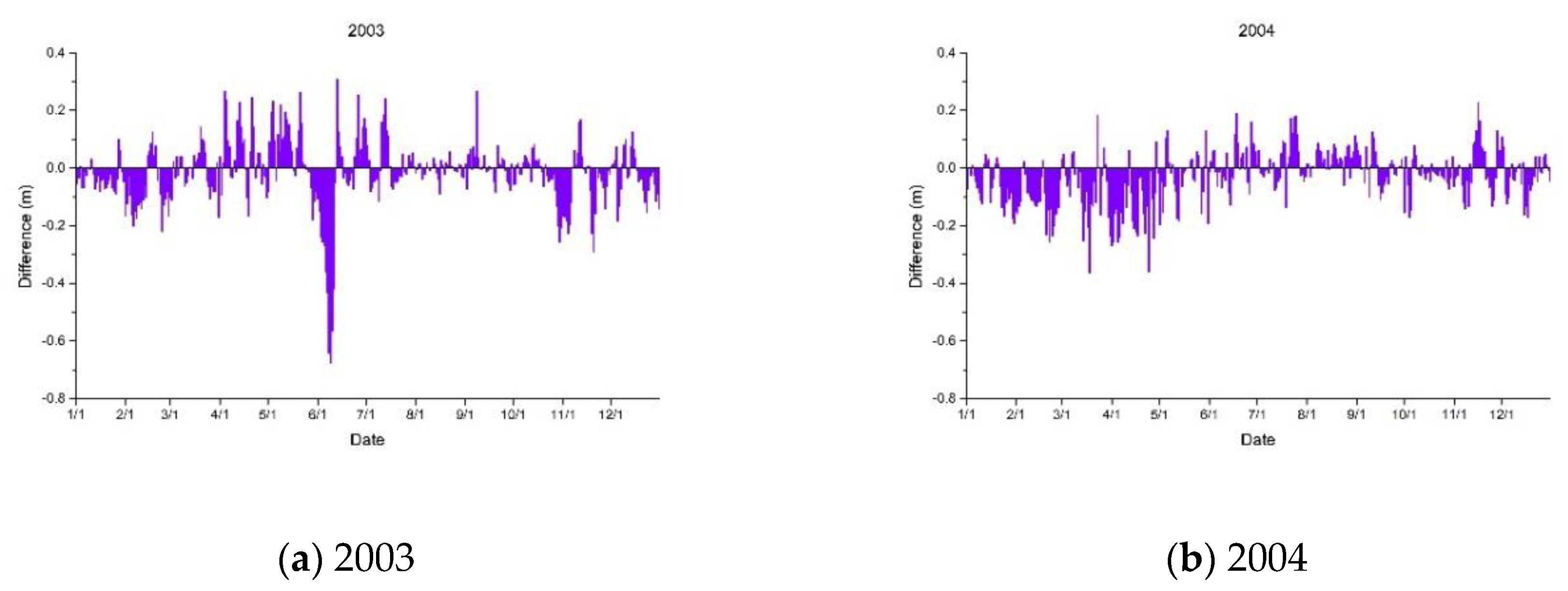
If we changed the TGD discharge variable and keep the other variables fixed, we could separate the TGD discharge impact from the complicated system and determine how it influenced the water level of Dongting Lake. We replaced the TGD discharge variable with the dam’s daily inflow data for the purpose of stimulating a situation where the TGD did not exist and determined how the water level of Dongting Lake changed accordingly [48]. We called this the mock data. The mock data included the inflow data of the TGD from 2003 to 2013, and the other variables were the same as before. We put the mock data into the LSTM network and obtained predictions for the water level of Dongting Lake from 2003 to 2013, and we called this result the mock water level. The difference was evaluated by subtracting the actual water level from the mock water level, which is shown in Figure 10.
In 2003, as shown in Figure 10a, large disparities appear in June. The water level dropped significantly in June compared to the mock data. This was because the TGD started its first impoundment in June 2003 until the water level of the dam reached 135 m at the end of June [49]. That time is when the TGD began to be actively used and started its first phase of operation. Based on this simulation experiment, the water level of Dongting Lake dropped 0.31 m on average during the TGD impoundment in June, and the largest drop on a single day was up to 0.65 m. There was also a noticeable drop in the water levels of Dongting Lake in November 2003 because the TGD impounded water again at that time, which enabled the dam water level to reach 139 m.
Through 2004 and 2005, the TGD did not operate regularly, so the impact on the water level variation was not large. Figure 10b,c shows that the water level of Dongting Lake dropped in the first half of the year in 2004 and 2005, and the water level rose slightly in the second half of the year in 2005.
In September 2006, the TGD started its second phase of operation, pushing the dam water level to 156 m. The impounding process lasted from September until the end of October, during which time there was a major drop in the water level of Dongting Lake, as shown in Figure 10d. The water level of Dongting Lake dropped 0.26 m on average according to the simulation experiment, and on extreme occasions, the drop was as much as 0.66 m.
In 2007, as illustrated in Figure 10e, the water level of Dongting Lake had a relatively large drop in July and August due to the flood control dispatch of the TGD.
In 2008, as shown in Figure 10f, there was a sharp drop in the water level in October and November. The reason for this decline is that the TGD implemented its third phase of operation, and the impounding process completed the goal of reaching the 175 m reservoir water level. Accordingly, the Dongting Lake water level dropped by 0.34 m on average during that time, and the largest drop in a single day was as much as 0.86 m.
In 2009, there was a relatively large increase around March as a result of the TGD’s water replenishment strategy during dry seasons. The water level of Dongting Lake showed a substantial drop in October and November because of the impoundment of the TGD (see Figure 10g).
In 2010, as we can see in Figure 10h, the water level variation was different from before, and what makes this year special was that the Yangtze River experienced one of the largest floods during summer. The flood peak in July was the third largest flood peak ever recorded in the Yangtze River hydrological record, and the flood reached more than 70,000 m3 flow per second [50]. Nevertheless, the water level of Dongting Lake did not increase much as a result. In fact, the lake level dropped 0.22 m after the TGD discharge was reduced to 30000 m3/s (maximum outflow), as opposed to 70000 m3/s (maximum inflow) if the TGD does not exist. The water level increased substantially in August after the flood, which was when the TGD opened sluices to release the flood water. By doing so, the TGD managed to stagger the flood peak to alleviate the rise in water level in Dongting Lake. Then, the water level showed a moderate decline in September and November due to the impoundment of the TGD.
In 2011, there was a mild increase in the water level for the first half of the year because of the dispatch of TGD water replenishment, which started on December 29, 2010, and ended on June 10, 2011. The replenishment raised the water level by 0.16 m on average, and the largest increase reached 0.3 m in the experiment (see Figure 10i). There was a drastic drop in September and October because the TGD was impounding water in order for the dam water level to reach 175 m again, and the drop was as much as 1.2 m.
In 2012, the water level of Dongting Lake increased slightly from January to June due to TGD water replenishment, and the peak increase was 0.48 m (see Figure 10j). Similar to 2010, the Yangtze River observed a large flood again in July, but the water level of Dongting Lake declined by 0.15 m during the first flood peak. Then, the water level rose considerably in August when the TGD opened the sluice and released the flood water. The water level dropped again in the fall because of the TGD impoundment, and the dam water level reached 175 m again on October 30.
In 2013, the water level of Dongting Lake showed a steady increase in the first quarter of the year with an average increase of 0.15 m due to the TGD water replenishment, and the lake showed some mild, intermittent decreases during wet seasons (see Figure 10k). There was a major decline from September to November when the TGD entered its impounding period until the reservoir water level again reached 175 m, and the largest drop of 0.75 m occurred on a single day.
5. Conclusions
In this article, a deep learning model based on an LSTM network was proposed to predict the daily water level of Dongting Lake. Seven variables were selected as input factors quintessential to the water level variations, and eight years of daily data (from 2003 to 2012) were used to train the model. Then, the model was tested on the daily data for the next three years (from 2011 to 2013). The experiments showed that the LSTM model predicted the water level of Dongting Lake with high precision and delivered better results compared to an SVM model.
This LSTM prediction model also established the connections between the water level of Dongting Lake and the TGD discharge. Eleven years of mock data (from 2003 to 2013) were used to simulate a situation where the TGD does not exist to examine how the water level of Dongting Lake differed from reality. Through this experiment, we made the following conclusions:
- The water level of Dongting Lake dropped conspicuously when the TGD is being impounded, which occurred annually from September to November. The drop was approximately 0.3 m on average and could be as large as 1.2 m in a single day.
- The water level increased mildly during dry seasons because of the TGD water replenishment strategy, which demonstrated the water conservancy effects of the dam.
- There was a decline in the water level of Dongting Lake during flood seasons (mostly July during flood peaks) and a lagged increase occurred later, proving that the dam’s effects on flood control and staggering the flood peak.
Overall, the TGD discharge control and its water regulation plans had a strong impact on the water level variation of Dongting Lake. With the forecasting model proposed in this article, the daily water level of Dongting Lake could be predicted, which will help with flood control and water regulation.
Author Contributions
C.L. collected data, and conceived and designed the study with the support of Q.D. C.L., H.L., M.L. and Q.D. drafted and revised the article together. All authors read and approved the final manuscript.
Funding
This research was funded by the National Key Research and Development Program of China (2016YFC0803106).
Acknowledgments
The authors would like to thank Qingyun Du from Wuhan University for his valuable suggestions. This work was supported by the National Key R&D Program of China (2016YFC0803106).
Conflicts of Interest
The authors declare no conflict of interest.
References
- Beeton, A.M. Large freshwater lakes: Present state, trends, and future. Environ. Conserv. 2002, 29, 21–38. [Google Scholar] [CrossRef]
- Yuan, Y.; Zhang, C.; Zeng, G.; Liang, J.; Guo, S.; Huang, L.; Wu, H.; Hua, S. Quantitative assessment of the contribution of climate variability and human activity to streamflow alteration in Dongting Lake, China. Hydrol. Processes 2016, 30, 1929–1939. [Google Scholar] [CrossRef]
- Mitsch, W.J.; Gosselink, J.G. Wetlands, 4th ed.; John Wiley & Sons Ltd.: New York, NY, USA, 2007. [Google Scholar]
- Yuan, Y.; Zeng, G.; Liang, J.; Huang, L.; Hua, S.; Li, F.; Zhu, Y.; Wu, H.; Liu, J.; He, X. Variation of water level in Dongting Lake over a 50-year period: Implications for the impacts of anthropogenic and climatic factors. J. Hydrol. 2015, 525, 450–456. [Google Scholar] [CrossRef]
- Hayashi, S.; Murakami, S.; Xu, K.-Q.; Watanabe, M. Effect of the Three Gorges Dam Project on flood control in the Dongting Lake area, China, in a 1998-type flood. J. Hydro-Environ. Res. 2008, 2, 148–163. [Google Scholar] [CrossRef]
- Jiang, L.; Ban, X.; Wang, X.; Cai, X. Assessment of hydrologic alterations caused by the Three Gorges Dam in the middle and lower reaches of Yangtze River, China. Water 2014, 6, 1419–1434. [Google Scholar] [CrossRef]
- Nakayama, T.; Shankman, D. Impact of the Three-Gorges Dam and water transfer project on Changjiang floods. Glob. Planet. Chang. 2013, 100, 38–50. [Google Scholar] [CrossRef]
- Guo, H.; Hu, Q.; Zhang, Q.; Feng, S. Effects of the Three Gorges Dam on Yangtze River flow and river interaction with Poyang Lake, China: 2003–2008. J. Hydrol. 2012, 416–417, 19–27. [Google Scholar] [CrossRef]
- Hu, Q.; Feng, S.; Guo, H.; Chen, G.; Jiang, T. Interactions of the Yangtze river flow and hydrologic processes of the Poyang Lake, China. J. Hydrol. 2007, 347, 90–100. [Google Scholar] [CrossRef]
- Zhou, J.; Peng, T.; Zhang, C.; Sun, N. Data pre-analysis and ensemble of various artificial neural networks for monthly streamflow forecasting. Water 2018, 10, 628. [Google Scholar] [CrossRef]
- Yu, Y.; Zhang, H.; Singh, V. Forward prediction of runoff data in data-scarce basins with an improved Ensemble Empirical Mode Decomposition (EEMD) model. Water 2018, 10, 388. [Google Scholar] [CrossRef]
- Delgado-Ramos, F.; Hervás-Gámez, C. Simple and low-cost procedure for monthly and yearly streamflow forecasts during the current hydrological year. Water 2018, 10, 1038. [Google Scholar] [CrossRef]
- Lai, X.J.; Jiang, J.H.; Huang, Q. Effect of Three Gorge Reservoir on the water regime of the Dongting Lake during important regulation periods. Resour. Environ. Yangtze Basin 2011, 20, 167–172. [Google Scholar]
- Wu, N.; Luo, Y.; Liu, T.; Huang, Z. Experimental study on the effect of the Three Gorges Project on water level in Lake Poyang. J. Lake Sci. 2014, 26, 522–528. [Google Scholar] [CrossRef] [Green Version]
- Jiang, J.; Huang, Q. Study on impacts of the Three Gorge Project on water level of Dongting Lake. Resour. Environ. Yangtze Basin 1996, 5, 367–374. [Google Scholar]
- Liu, Z.; Zhou, P.; Chen, X.; Guan, Y. A multivariate conditional model for streamflow prediction and spatial precipitation refinement. J. Geophys. Res. Atmos. 2015, 120, 10116–10129. [Google Scholar] [CrossRef]
- Khedun, C.P.; Mishra, A.K.; Singh, V.P.; Giardino, J.R. A copula-based precipitation forecasting model: Investigating the interdecadal modulation of ENSO’s impacts on monthly precipitation. Water Resour. Res. 2014, 50, 580–600. [Google Scholar] [CrossRef]
- Liu, Z.; Zhou, P.; Zhang, Y. A Probabilistic Wavelet-Support Vector Regression Model for Streamflow Forecasting with Rainfall and Climate Information Input. J. Hydrometeorol. 2015, 16, 2209–2229. [Google Scholar] [CrossRef]
- Coulibaly, P. Reservoir Computing approach to Great Lakes water level forecasting. J. Hydrol. 2010, 381, 76–88. [Google Scholar] [CrossRef]
- Coppola, E.; Szidarovszky, F.; Poulton, M.; Charles, E. Artificial neural network approach for predicting transient water levels in a multilayered groundwater system under variable state, pumping, and climate conditions. J. Hydrol. Eng. 2003, 8, 348–360. [Google Scholar] [CrossRef]
- Wang, M.; Dai, L.; Dai, H.; Mao, J.; Liang, L. Support vector regression based model for predicting water level of Dongting Lake. J. Drain. Irrig. Mach. Eng. 2017, 35, 954–961. [Google Scholar] [CrossRef]
- Chen, Y.; Fan, R.; Yang, X.; Wang, J.; Latif, A. Extraction of urban water bodies from high-resolution remote-sensing imagery using deep learning. Water 2018, 10, 585. [Google Scholar] [CrossRef]
- LeCun, Y.; Bengio, Y.; Hinton, G. Deep learning. Nature 2015, 521, 436. [Google Scholar] [CrossRef] [PubMed]
- Ding, X.; Li, X. Monitoring of the water-area variations of Lake Dongting in China with ENVISAT ASAR images. Int. J. Appl. Earth Obs. Geoinf. 2011, 13, 894–901. [Google Scholar] [CrossRef]
- Li, F.; Huang, J.; Zeng, G.; Yuan, X.; Li, X.; Liang, J.; Wang, X.; Tang, X.; Bai, B. Spatial risk assessment and sources identification of heavy metals in surface sediments from the Dongting Lake, Middle China. J. Geochem. Explor. 2013, 132, 75–83. [Google Scholar] [CrossRef]
- Li, Y.; Yang, G.; Li, B.; Wan, R.; Duan, W.; He, Z. Quantifying the effects of channel change on the discharge diversion of Jingjiang Three Outlets after the operation of the Three Gorges Dam. Hydrol. Res. 2016, 47. [Google Scholar] [CrossRef]
- Qin, H. The Succession and Reason Analysis of Hydrological Environment in the Dongting Lake in Recent 50 Years; Hunan Agricultural University: Changsha, China, 2013. [Google Scholar]
- Shi, X.; Xiao, W.; Wang, Y.; Wang, X. Characteristics and factors of water level variations in the Dongting Lake during the recent 50 years. South-to-North Water Transf. Water Sci. Technol. 2012, 10, 18–22. [Google Scholar] [CrossRef]
- Yang, Y.; Zhang, M.; Zhu, L.; Liu, W.; Han, J.; Yang, Y. Influence of large reservoir operation on water-levels and flows in reaches below dam: Case study of the Three Gorges Reservoir. Sci. Rep. 2017, 7, 15640. [Google Scholar] [CrossRef] [PubMed]
- Zhang, J.; Feng, L.; Chen, L.; Wang, D.; Dai, M.; Xu, W.; Yan, T. Water compensation and its implication of the Three Gorges Reservoir for the river-lake system in the middle Yangtze River, China. Water 2018, 10, 1011. [Google Scholar] [CrossRef]
- Fausett, L. Fundamentals of Neural Networks: Architectures, Algorithms, and Applications; Prentice-Hall: Upper Saddle River, NJ, USA, 1994. [Google Scholar]
- Graves, A. Supervised Sequence Labelling with Recurrent Neural Networks; Springer: Berlin/Heidelberg, Germany; London, UK, 2012. [Google Scholar]
- Bengio, Y.; Simard, P.; Frasconi, P. Learning long-term dependencies with gradient descent is difficult. IEEE Trans. Neural Netw. 1994, 5, 157–166. [Google Scholar] [CrossRef] [PubMed]
- Hochreiter, S.; Schmidhuber, J. Long Short-Term Memory. Neural Comput. 1997, 9, 1735–1780. [Google Scholar] [CrossRef] [PubMed]
- Ke, J.; Zheng, H.; Yang, H.; Chen, X. Short-term forecasting of passenger demand under on-demand ride services: A spatio-temporal deep learning approach. Transp. Res. C-Emerg. 2017, 85, 591–608. [Google Scholar] [CrossRef] [Green Version]
- Chemali, E.; Kollmeyer, P.J.; Preindl, M.; Ahmed, R.; Emadi, A. Long short-term memory networks for accurate state-of-charge estimation of Li-ion batteries. IEEE Trans. Ind. Electron. 2018, 65, 6730–6739. [Google Scholar] [CrossRef]
- Han, Q.; Zhang, S.; Huang, G.; Zhang, R. Analysis of long-term water level variation in Dongting Lake, China. Water 2016, 8, 306. [Google Scholar] [CrossRef]
- Arce, M.E.; Saavedra, Á.; Míguez, J.L.; Granada, E. The use of grey-based methods in multi-criteria decision analysis for the evaluation of sustainable energy systems: A review. Renew. Sustain. Energy Rev. 2015, 47, 924–932. [Google Scholar] [CrossRef]
- Tzeng, C.-J.; Lin, Y.-H.; Yang, Y.-K.; Jeng, M.-C. Optimization of turning operations with multiple performance characteristics using the Taguchi method and Grey relational analysis. J. Mater. Process. Technol. 2009, 209, 2753–2759. [Google Scholar] [CrossRef]
- Kreyszig, E. Advanced Engineering Mathematics, 4th ed.; Wiley: New York, NY, USA, 1979. [Google Scholar]
- Huang, L.; Hung, S.; Leu, J. A Study on the Effects of Rolling Forecast with Different Information Sharing Models on Supply Chain Performance. In Proceedings of the 40th International Conference on Computers & Indutrial Engineering, Awaji Island, Japan, 25–28 July 2010; pp. 1–6. [Google Scholar]
- Ruder, S. An overview of gradient descent optimization algorithms. arXiv, 2016; arXiv:1609.04747. [Google Scholar]
- Behzad, M.; Asghari, K.; Coppola, E.A. Comparative study of SVMs and ANNs in aquifer water level prediction. J. Comput. Civ. Eng. 2010, 24, 408–413. [Google Scholar] [CrossRef]
- Dibike, Y.B.; Velickov, S.; Solomatine, D.; Abbott, M.B. Model induction with support vector machines: Introduction and applications. J. Comput. Civ. Eng. 2001, 15, 208–216. [Google Scholar] [CrossRef]
- Kim, K.-J. Financial time series forecasting using support vector machines. Neurocomputing 2003, 55, 307–319. [Google Scholar] [CrossRef]
- Thissen, U.; van Brakel, R.; de Weijer, A.P.; Melssen, W.J.; Buydens, L.M.C. Using support vector machines for time series prediction. Chemometrics Intell. Lab. Syst. 2003, 69, 35–49. [Google Scholar] [CrossRef]
- Tayfur, G.; Singh, V.; Moramarco, T.; Barbetta, S. Flood hydrograph prediction using machine learning methods. Water 2018, 10, 968. [Google Scholar] [CrossRef]
- Huang, Q.; Sun, Z.; Jiang, J. Impacts of the operation of the Three Gorges Reservoir on the lake water level of Lake Dongting. J. Lake Sci. 2011, 23, 424–428. [Google Scholar] [CrossRef] [Green Version]
- Gao, B.; Yang, D.; Yang, H. Impact of the Three Gorges Dam on flow regime in the middle and lower Yangtze River. Quat. Int. 2013, 304, 43–50. [Google Scholar] [CrossRef]
- Lai, X.-J.; Wang, Z.-M. Flood management of Dongting Lake after operation of Three Gorges Dam. Water Sci. Eng. 2017, 10, 303–310. [Google Scholar] [CrossRef]
Figure 1.
River–lake system of Dongting Lake.

Figure 2.
Structure of the LSTM network.

Figure 3.
Data display of the selected variables.

Figure 4.
Box-and-whisker plot for activation function selection.

Figure 5.
Box-and-whisker plot for optimization algorithm selection.

Figure 6.
Box-and-whisker plot for layer number selection.

Figure 7.
Forecasting results of the Dongting Lake water level using the LSTM model.

Figure 8.
Forecasting results of Dongting Lake water levels using the SVM model.

Figure 9.
Model performances in different water level ranges.

Figure 10.
Water level difference between reality and simulation every year with (a–k) showing years 2003–2013, respectively.
Figure 10.
Water level difference between reality and simulation every year with (a–k) showing years 2003–2013, respectively.


Table 1.
GRA results.
| Variables | TGD discharge | Xiangtan discharge | Taojiang discharge | Taoyuan discharge | Jinshi discharge | Precipitation |
| Grey relational grade | 0.7242 | 0.6699 | 0.6798 | 0.6570 | 0.6140 | 0.6197 |
Table 2.
Selected variables.
| Var 1 | Var 2 | Var 3 | Var 4 | Var 5 | Var 6 | Var 7 |
|---|---|---|---|---|---|---|
| Water level | TGD discharge | Xiangtan discharge | Taojiang discharge | Taoyuan discharge | Jinshi discharge | Precipitation |
Table 3.
Converting variables to a supervised dataset for the LSTM network.
| Var1 (t − 1) 1 | Var2 (t − 1) | Var3 (t − 1) | Var4 (t − 1) | Var5 (t − 1) | Var6 (t − 1) | Var7 (t − 1) | Var1 (t) |
|---|---|---|---|---|---|---|---|
| Water level | TGD discharge | Xiangtan discharge | Taojiang discharge | Taoyuan discharge | Jinshi discharge | Precipitation | Water level |
1 Var1 (t − 1) refers to variable 1 at time t − 1, and the same is true for the other variables.
Table 4.
Test results of running the LSTM model 10 times on the test dataset.
| No. | RMSE | R2 |
|---|---|---|
| 1 | 0.083 | 0.999 |
| 2 | 0.091 | 0.999 |
| 3 | 0.099 | 0.999 |
| 4 | 0.090 | 0.999 |
| 5 | 0.086 | 0.999 |
| 6 | 0.086 | 0.999 |
| 7 | 0.085 | 0.999 |
| 8 | 0.085 | 0.999 |
| 9 | 0.088 | 0.999 |
| 10 | 0.087 | 0.999 |
Table 5.
Input and output variables for the SVM model.
| Input | Output | |||||
|---|---|---|---|---|---|---|
| Var1 | Var2 | Var3 | Var4 | Var5 | Var6 | Target variable |
| TGD discharge | Xiangtan discharge | Taojiang discharge | Taoyuan discharge | Jinshi discharge | Precipitation | Water level |
© 2018 by the authors. Licensee MDPI, Basel, Switzerland. This article is an open access article distributed under the terms and conditions of the Creative Commons Attribution (CC BY) license (http://creativecommons.org/licenses/by/4.0/).
Share and Cite
MDPI and ACS Style
Liang, C.; Li, H.; Lei, M.; Du, Q. Dongting Lake Water Level Forecast and Its Relationship with the Three Gorges Dam Based on a Long Short-Term Memory Network. Water 2018, 10, 1389. https://doi.org/10.3390/w10101389
AMA Style
Liang C, Li H, Lei M, Du Q. Dongting Lake Water Level Forecast and Its Relationship with the Three Gorges Dam Based on a Long Short-Term Memory Network. Water. 2018; 10(10):1389. https://doi.org/10.3390/w10101389
Chicago/Turabian StyleLiang, Chen, Hongqing Li, Mingjun Lei, and Qingyun Du. 2018. "Dongting Lake Water Level Forecast and Its Relationship with the Three Gorges Dam Based on a Long Short-Term Memory Network" Water 10, no. 10: 1389. https://doi.org/10.3390/w10101389
Note that from the first issue of 2016, this journal uses article numbers instead of page numbers. See further details here.