Multi-Objective Parameter Estimation of Improved Muskingum Model by Wolf Pack Algorithm and Its Application in Upper Hanjiang River, China

Abstract

In order to overcome the problems in the parameter estimation of the Muskingum model, this paper introduces a new swarm intelligence optimization algorithm—Wolf Pack Algorithm (WPA). A new multi-objective function is designed by considering the weighted sum of absolute difference (SAD) and determination coefficient of the flood process. The WPA, its solving steps of calibration, and the model parameters are designed emphatically based on the basic principle of the algorithm. The performance of this algorithm is compared to the Trial Algorithm (TA) and Particle Swarm Optimization (PSO). Results of the application of these approaches with actual data from the downstream of Ankang River in Hanjiang River indicate that the WPA has a higher precision than other techniques and, thus, the WPA is an efficient alternative technique to estimate the parameters of the Muskingum model. The research results provide a new method for the parameter estimation of the Muskingum model, which is of great practical significance to improving the accuracy of river channel flood routing.

1. Introduction

In recent years, frequent floods have caused serious losses to people’s lives and property [1]. Therefore, it is urgent to identify the flood routing rules to reduce flood losses. As a classic solution of flood routing, the Muskingum model continues to be a popular method for flood routing [2]. The Muskingum model was first developed by McCarthy [3]. In practical application, the key problem for applying the Muskingum model is parameter estimation [4,5], which is a highly nonlinear optimization problem. The studies on the Muskingum model mainly include the parameter estimation method and model improvement.

Traditional parameter estimation methods mainly include the Trial Algorithm (TA), the moment method, the least squares method, and the differential algorithm [5,6]. However, these methods are limited by the optimal estimation of the channel storage curve, which has led to a significant error between the calculated results and the observed data. In recent years, intelligence algorithms have been widely used in solving the nonlinear problem accurately and efficiently [7]. Many researchers have applied various techniques to estimate the parameters of the Muskingum model in recent years. For example, Luo and Xie [4] applied the immune clonal selection algorithm to estimate the parameters of the Muskingum model, getting a higher precision than the other techniques. Mohon [8] proposed the genetic algorithm to estimate the parameters of two nonlinear Muskingum routing models. Chen and Yang [9] applied the Gray-encoded accelerating genetic algorithm in the parameters optimization of the Muskingum model. Chu and Chang [10] used the Particle Swarm Optimization (PSO) algorithm to estimate the Muskingum model parameters, which improves the accuracy of the Muskingum model for flood routing. Barati [11] applied the parameter-setting-free technique, interfaced with a harmony search algorithm to the parameter estimation of the Muskingum model, and found good model parameter values. Zhang et al. [12] applied the Shuffle Complex Evolution Algorithm (SCE-UA) to optimize and estimate the discharge proportion coefficient x of the Muskingum equation and the number of streams subsections partitioned for mainstreams and tributaries. Niazkar and Afzali [13] proposed a hybrid method, which combined the Modified Honey Bee Mating Optimization and Generalized Reduced Gradient algorithms, reducing the sum of the squared (SSQ) value for the double-peak case study. Ouyang et al. [14] applied the invasive weed optimization (HIWO) algorithm to the parameter estimation of nonlinear Muskingum models. Although various techniques were applied to estimate the parameters of the nonlinear Muskingum flood routing model, the application of the model still suffers from a lack of an efficient method for parameter estimation. An efficient method for parameter estimation in the Muskingum model is still required to improve computational precision.

The improved Muskingum model mainly includes parameter setting and optimization criteria [15,16], and studies on model improvement have had a significant breakthrough in recent years. Zhang et al. and Vatankhah [17,18], for example, used a nonlinear Muskingum flood routing model with variable exponent parameters, producing the most accurate fit for outflow data. Moghaddam et al. [19] proposed a new Muskingum model with four parameters, the sum of the squared (SSQ) or absolute (SAD) deviations between the observed and estimated outflows considered as objective functions. Although the new Muskingum model becomes more complex, it improves the fit to observed flow, especially in multiple-peak hydrographs. Luo et al. [20] proposed a multi-objective estimation routine of the Muskingum model, involving single-peak, multi-peak, and non-smooth hydrographs, proving that the multi-objective estimation procedure is consistent and effective in estimating the parameters of the Muskingum model. Easa [21] pointed out models that adopt the outflow criterion result in a poor fit to the observed storages, presenting a new approach that incorporates both criteria in the estimation process and aids trade-off analysis.

This paper proposes a parameter estimation of the Muskingum model based on a new intelligent algorithm—the Wolf Pack Algorithm (WPA). In this paper, several floods with different magnitudes from river channels (Ankang hydropower station–Ankang city and Ankang hydropower station–Shuhe) of the Hanjiang River were first selected to estimate their respective parameters. Secondly, an improved multi-objective of the Muskingum model as well as that of the WPA and its solving steps are proposed. Thirdly, the results from the different algorithms in terms of the weighted sum of absolute difference and the coefficient of determination between the observed and routed outflows are compared to verify the performance of the WPA. Finally, conclusions are drawn based on the results.

2. Materials and Methods

2.1. Research Area

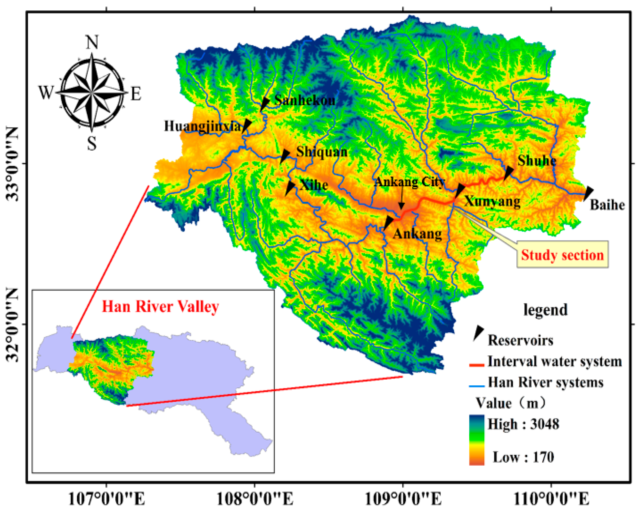
The Ankang to Shuhe section of Hanjiang River in China was chosen as the study area (Figure 1). The length of the river section is 109.36 km, accounting for 7% of the total reach of the Han River, with a drop of 61 m and an average gradient ratio of 0.06% of the river bed. Due to the steep slope of the mountain basin, the poor permeability of the rock formation, and poor adjustment of the channel, the flood process is very fast, the peak shape is thin, the inter-annual variability of the flood is larger, and the flood variation coefficient is larger. The parameters of the river and flood data are shown in

Table 1. Data of river section.

Reach	Height Difference (m)	River Length (km)	Gradient (%)
Ankang Reservoir–Ankang city (Reach 1)	11.24	18.31	0.06
Ankang Reservoir–Shuhe Reservoir (Reach 2)	61.00	109.00	0.06

and

Table 2. Data of flood.

Reach	Flood Event	Flood Peak (m3/s)	Total Amount of Floods (108 m3)	Flood Peak Time (h)
Ankang Reservoir–Ankang city	20100821	7260	173	1
	20120707	8420	241	1
	20120901	7645	171	1
Ankang Reservoir–Shuhe Reservoir	20130722	7178	44	7
	20140909	7607	67	6
	20140914	6637	52	7

.

2.2. Muskingum Model

2.2.1. Model Basic Principle

The Muskingum model is a traditional method for solving river flood routing, which is mainly solved by the continuity equation and the dynamic equation [22]. In order to obtain the flood routing equation, the water balance equation and storage equation are solved by:

$$Q_2=C_0{I}_2+C_1{I}_1+C_2{Q}_1$$

(1)

$$\{\begin{array}{l}{C}_0=\frac{-Kx+0.5\Delta t}{K-Kx+0.5\Delta t}\\ C_1=\frac{Kx+0.5\Delta t}{K-Kx+0.5\Delta t}\\ C_2=\frac{K-Kx-0.5\Delta t}{K-Kx+0.5\Delta t}\end{array}$$

(2)

where $Q_1$ and $Q_2$ are the outflow of the downstream section at the beginning and the end of the period, respectively, $I_1$ and $I_2$ are the inflow of upstream section at the beginning and the end of the period, $K$ is channel storage coefficient, and $x$ is specific gravity coefficient of flow. $C_0$, $C_1$, and $C_2$ are the flow routing coefficients.

2.2.2. Design of Objective Function

The optional parameters of the Muskingum model can be $x$ and $K$, or $C_0$, $C_1$, and $C_2$. If $K$ and $x$ are chosen as the optimization variables, it is necessary to ensure that the water storage capacity of the river is a single linear relationship with the reservoir flow during the optimization process, which is difficult to determine, given the range of variables. Meanwhile, there is no need to go deep into the physical parameters of the model, because of the intelligent algorithm based on the black box model [23]. Therefore, $C_0$ and $C_1$ are chosen as the optimization variables. The results of river flood routing are mainly reflected in the flood process and the flood peak of the simulation.

The results of river flood flow evolution are mainly reflected in the degree of fitting of flood process and flood peak to the actual flood. Some studies indicated that the success of a calibration process is highly dependent on the objective function chosen as a calibration criterion [19]. The most commonly used objective function for the calibration procedure is the SSQ errors between observed and computed outflow [4,5,20,24], but some research has indicated that the SSQ is not necessarily correct [16,25]. Considering the above reasons, the objective function established in this paper can be described as follows:

Objective 1: Minimum weighted sum of absolute difference (SAD):

$$f_1=\min {\displaystyle \sum _{i=2}^n}\left[Q_0(i)\left|C_0{I}_c(i)+C_1{I}_c(i-1)+C_2{Q}_0(i-1)-Q_0(i)\right|\right]$$

(3)

$$\begin{array}{lll}s.t.:& & C_0\in [-1,1]\\ & & C_1\in [-1,1]\\ & & C_2=1-C_0-C_1\in [-1,1]\end{array}$$

(4)

where $Q_0(i)$ is the actual outflow of the downstream section at a time $i$, $I_c(i-1)$ and $I_c(i)$ are the simulated flow for the upstream section at time $(i-1)$ and $i$, respectively, $Q_0(i-1)$ is the simulated flow for the upstream section at time $(i-1)$, and n is the length of the time series used for calibration. $C_0$, $C_1$, and $C_2$ are the flow routing coefficients.

The SAD will give the minimum difference between observed and computed outflow [9,19,26]. Objective 1 is the SAD multiplying the corresponding weight taken from the observed flow at the corresponding time, which will increase large flow influence on the parameter estimation, especially on the flood peak. Thus, the weight can increase the simulation accuracy of the flood peak.

Objective 2: Maximum coefficient of determination $D_c$:

$$f_2=\max D_c=\max \left[1-\frac{{\displaystyle \sum _{i=1}^n}{(Q_c(i)-Q_0(i))}^2}{{\displaystyle \sum _{i=1}^n}{(Q_0(i)-{\overline{Q}}_0)}^2}\right]$$

(5)

where $D_c$ is the coefficient of determination, $Q_c(i)$ is the computed value at time $i$, $Q_0(i)$ is the observed value at time $i$, ${\overline{Q}}_0$ is the mean value of the observed flood process, and $n$ is the number of time series used for calibration [22].

The deterministic coefficient is an indicator to measure the consistency between the flood forecast and the observed process. In this paper, the coefficient of determination as Objective 2 can ensure that the simulated flow process is the closest to the observed values [27,28].

In order to reduce the multi-objective calculation and adaptation algorithm, the comprehensive multi-objective function chosen in this paper is as follows:

$$f=\max ({\varphi }_1(-f_1)+{\varphi }_2{f}_2)$$

(6)

where $f$ is the comprehensive objective, $f_1$ and $f_2$ are Objective 1 and Objective 2, respectively, and ${\varphi }_1$ and ${\varphi }_2$ are the weight coefficient of different objectives, respectively.

3. Methodology

3.1. Wolf Pack Algorithm (WPA)

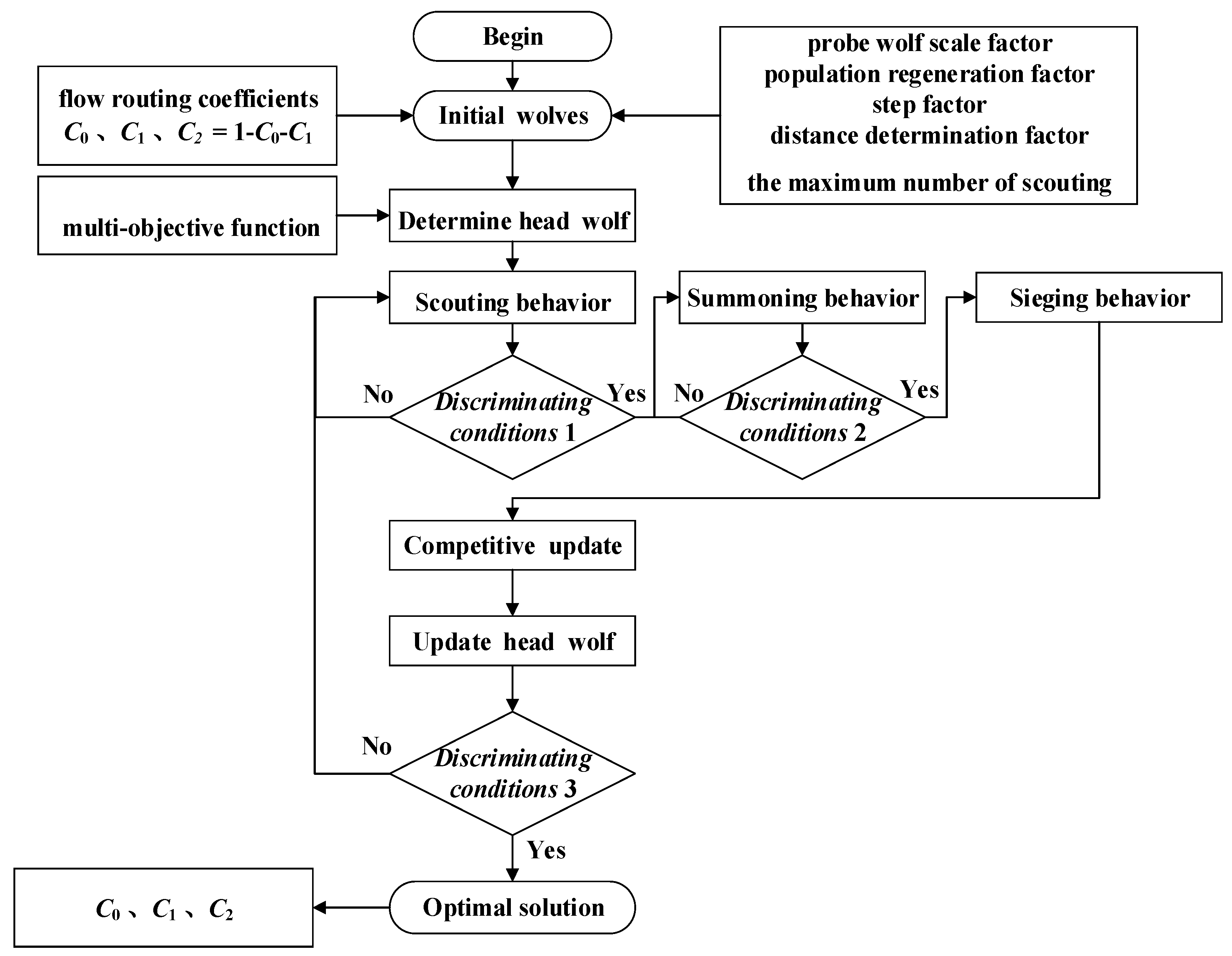
The Wolf Pack Algorithm is a novel swarm intelligence algorithm with strong local search ability and global convergence. It consists of the leading wolf, fierce wolves, and explore wolves, including three kinds of intelligent behaviors: Scouting, summoning, and beleaguering. Simultaneously, with a productive rule for the leading wolf, which is that the winner can dominate all, it is a renewable mechanism, namely survival of the fittest, for a pack of wolves. It has been applied in the field of mathematics, physics, and hydropower station optimization, achieving good calculation results [29,30,31]. In this paper, the WPA is used for the parameter estimation of the Muskingum model. Combining the principle of the WPA with the objective function, we designed a WPA for solving Muskingum model parameters. The procedure of our algorithm for parameter optimal estimation of the Muskingum model is shown as follows:

Step 1: (Initial wolves) We must initially determine the size of the algorithm population $n$ and the number of iterations $gen$, the probe wolf scale factor $a$, the population regeneration factor $b$, the step factor $S$, the distance determination factor $W$, and the maximum number of scouting $T_{\max }$. The Model Parameter $(C_0,C_1)$ is regarded as the position of the artificial wolf $(x_1,x_2)$ in a two-dimensional decision space. The position of the wolf pack is initialized in the range of $C_0$ and $C_1$, as shown in Equation (7):

$$\begin{array}{ccc}{x}_{i,j}=2\times rand-1& & i=1,2,\dots ,n;j=1,2\end{array}$$

(7)

where $x_{i,j}$ is the initial position of the i-th wolf in the j-th decision space; $rand$ is a uniformly distributed random number in the interval [0,1].

Step 2: (Scouting) Choose the objective function f as the prey odor concentration $Y_t(i)$ and calculate the prey odor concentration at the location of the artificial wolf. According to the $Y_t(i)$, sort all artificial wolf positions in descending order, then select the first artificial wolf of the sorted population as a head wolf, whose location is regarded as $x_{lead}$ and the prey odor concentration is $Y_{lead}$. Choose the second to $S+1$ artificial wolves as the explore wolves that total $S=Round(a\ast n)$, and the remaining artificial wolves as the fierce wolves. The explore wolves scout to conduct a fine search, until the maximum number of walks is reached or the maximum global optimal solution is found.

Step 3: (Summoning) The fierce wolfs quickly approach the head wolf to achieve the global convergence of solution, until the Euclidean distance $d_{is}(i)$ between all fierce wolves and the head wolf is less than the judgment value of distance ${d_{nea}}_r$ or a contemporary global optimal solution is found. The calculation formula of the distance judgment value is:

$${d_{nea}}_r=\frac{{\displaystyle \sum _{d=1}^D}\left|{\max }^d-{\min }^d\right|}{D\ast W}=\frac{2}{W}$$

(8)

where ${d_{nea}}_r$ is the judgment value of distance; $D$ is the spatial dimension; $W$ is the distance determining factor; ${\max }^d$, ${\min }^d$ are the upper and lower limits of the decision variable $x_{i,j}$, respectively.

Step 4: (Sieging) Under the command of the head wolf, other artificial wolves further update the location to achieve local fine optimization.

Step 5: (Competitive update) According to the population, update factor b, calculate the amount of the population, update $R$ and regenerate $R$ artificial wolves, which can be alternated with the previous generation of artificial wolves with a low fitness value to ensure the diversity of solutions and to avoid falling into the local optimal.

Step 6: Determine whether the maximum number of iterations has been reached; if it has, output the optimal global solution. If not, proceed to the next generation calculation and return to Step 2 until the maximum number of iterations is reached.

The WPA flow chart for solving the Muskingum model parameters is shown in Figure 2.

3.2. Parameter Sensitivity Analysis

The WPA involves a relatively large number of parameters; the main sensitivity parameters are the distance determination factor $W$ and the step factor $S$. Therefore, this paper focuses on the discussion of parameters $W$ and $S$ on the algorithm. In order to determine the distance determination factor $W$ and the step factor $S$, the parameters were set as follow: Artificial wolf population size $n=20$, explore wolf proportion factor $a=4$, population update factor $b=2$, the maximum number of scouting $T_{\max }=2$, the number of iterations $gen=30$. With the Muskingum principle, the algorithm is used to solve $D$-dimensional space problem $(D=2)$, and the upper and lower limits of the variables are ${\max }^d=1$ and ${\min }^d=-1$, respectively.

The WPA’s raid step:

$$ste{p}_b^d=\frac{2({\max }^d-{\min }^d)}{S}=\frac{4}{S}$$

(9)

where $ste{p}_b^d$ is the step size of the d-dimensional space; $S$ is the step factor; ${\max }^d$, ${\min }^d$ are the upper and lower limits of the decision variable $x_{i,j}$, respectively.

In the summoning act, the condition of the artificial wolf raid termination is $d_{is}<d_{near}$, so the rapid step should meet the following formula:

$${\displaystyle \sum _{d=1}^D}ste{p}_b^d<d_{near}$$

(10)

where the parameters are the same as above.

From Formula (10):

$$S>4W$$

(11)

where the parameters are the same as above.

From the above derivation, it can be seen that the normal operation of the algorithm can be satisfied when the step factor $S$ and the distance determination factor $W$ satisfy the formula (11).

Fixed distance determination factor $W=20$, set $S=100,105,110,115,120$, and 130, respectively. For each $S$, run the program code 20 times independently, select the evaluation index of the algorithm, the absolute deviation of the flood process, and the observed and simulated flood peak deviation. The absolute deviation of the flood process and the formula are as follow:

$$\delta ={\displaystyle \sum _{i=1}^n}\left|(Q_0(i)-Q_c(i))\right|$$

(12)

where $\delta$ is the absolute deviation of the flood process, m³/s.

The flood peak deviation is:

$$f=\frac{1}{n}{\displaystyle \sum _{i=1}^n}\left|(Q_{obs,i}^{peak}-Q_{sim,i}^{peak})\right|$$

(13)

where f is the flood peak deviation; $Q_{obs,i}^{peak}$ and $Q_{sim,i}^{peak}$ are the observed and simulated maximum outflow at peak flow event number i, respectively; n is the number of simulations times.

The evaluation index values are taken from the average of 20 independent runs. Taking the flood event of 20100821 as an example, the results are shown in

Table 3. Sensitivity analysis of step factor.

W	S	δ (m3/s)	Flood Peak Deviation (m3/s)
20	100	7892.7	6.33
	104	7892.4	6.31
	110	7891.9	6.29
	115	7891.7	6.29
	120	7891.6	6.29
	130	7891.6	6.29

.

As shown in Table 3:

(1) With the increase of the $S$ value, $\delta$ decreases slightly from 7892.7 m³/s to 7891.6 m³/s, which indicates that the larger the step size, the finer the search, and the closer the flood forecast results are to the actual flood process.

(2) When $W=20$, the variation range of $\delta$ and flood peak are not large, which indicates that the step size of the WPA has little influence on the forecast results in a certain range.

Keeping in mind that the smaller the searching step, the more time consuming the process is, the initial selection of $S=120$, that is $S=6W$. $W=20,30,40,50,60$, and 70 are selected to simulate the same flood, and the results are shown in

Table 4. Sensitivity analysis of distance judgment factor.

W	S	δ (m3/s)	Flood Peak Deviation (m3/s)
20	120	7891.6	6.29
30	180	7891.4	6.20
40	240	7891.2	6.20
50	300	7891.0	6.12
60	360	7890.8	6.12
70	420	7890.8	6.12

.

As shown in Table 4:

(1) With the increase of $W$, $\delta$ decreases slightly, and the minimum value appears at $W=60$. The peak deviation is also minimized, and then the $W$ value increases; the optimization effect has no obvious change.

(2) The range of $\delta$ is not significant, and indicates that the parameter $W$ of the wolves algorithm on the two-dimensional nonlinear optimization problem has little influence on the algorithm, and the algorithm is more applicable.

With the increase of $W$, the raid step will be smaller, and the optimization result is too fine, which will cause the artificial wolf to turn from difficult to besieging. Thus, the algorithm has the possibility of entering an infinite loop.

In order to further analyze the influence of different weight coefficients on the forecast results, we set different weight coefficients using the same method. The results are shown in

Table 5. Multi-objective weight coefficient analysis.

${\mathit{\varphi }}_{\mathbf{1}}$	${\mathit{\varphi }}_{\mathbf{2}}$	δ (m3/s)	Flood Peak Deviation (m3/s)
0.9	0.1	7916.9	6.16
0.8	0.2	7914.8	6.16
0.7	0.3	7912.9	6.18
0.6	0.4	7906.1	6.19
0.5	0.5	7901.0	6.19
0.4	0.6	7896.6	6.19
0.3	0.7	7891.1	6.20
0.2	0.8	7891.7	6.22
0.1	0.9	7891.6	6.26

.

As shown in Table 5:

(1) With the decrease of ${\varphi }_1$, peak deviation increased slightly, with an increase 0.1 m³/s only. When ${\varphi }_1$ is 0.8 or 0.9, the flood peak deviation takes the minimum, which indicated that the weight factor of Objective 1 focuses on the minimum deviation of flood peak.

(2) With the increase of ${\varphi }_2$, the absolute deviation of the flood process is gradually reduced from 7916.9 m³/s to 7891.6 m³/s, and reaches the minimum value when ${\varphi }_2$ is 0.7, which indicated that the weight factor of Objective 2 focuses on the total error of the entire flood process.

According to comprehensive analysis, the weight coefficient ${\varphi }_2$ had a great influence on the fitting effect of the whole flood process and ${\varphi }_1$ had little effect on the flood peak simulation. Therefore, ${\varphi }_1=0.3$ and ${\varphi }_2=0.7$ were selected for the multi-objective weight value.

4. Results and Discussion

In this paper, we took flood forecasting of Ankang hydropower station to Ankang city and Ankang hydropower station to Shuhe hydropower Station as examples. Considering the length of the two Reaches, the actual demand, and the characteristics of the inflow, the calculation time steps of Reach 1 and Reach 2 were 1 h and 6 h, respectively. The improved Muskingum method (WPA), Particle Swarm Optimization (PSO), and Trial Algorithm (TA) were selected to compare to the observed outflow. In the WPA, the values of distance determination (W) and the step (S) were both 100. The maximum number of iterations was 50. The value of the artificial wolf population size (n) was 20. The values of the explore wolf proportion (a) and population update (b) were 4 and 2, respectively. In the TA [22], the parameters (k, x) of this algorithm are shown in

Table 6. Parameter estimation results obtained from different methods.

Flood Event		20100821	20120707	20120901	20130722	20140909	20140914
TA	k	1.50	1.50	1.50	1.00	1.00	1.00
	x	0.10	0.10	0.10	0.20	0.20	0.20
PSO	k	0.21	1.18	0.88	1.48	1.37	1.17
	x	−4.17	0.23	−0.43	0.23	−0.42	0.11
WPA	k	0.58	1.23	0.86	1.46	1.56	1.20
	x	−0.88	0.24	−0.42	0.22	−0.68	0.12

. In the PSO algorithm, a population of 50 individuals was used. The maximum number of iterations in the program was 100. The values of the acceleration constants $c_1$ and $c_2$ were both set to 0.2.

The corresponding parameters estimated by the WPA, TA, and PSO are listed in Table 6. It can be seen from Table 6 that the parameters obtained from the three methods are all technically reasonable, but do show marked differences. The estimated value of the parameters differ very little between the WPA and PSO, but the parameters of TA vary quite significantly with WPS and PSO.

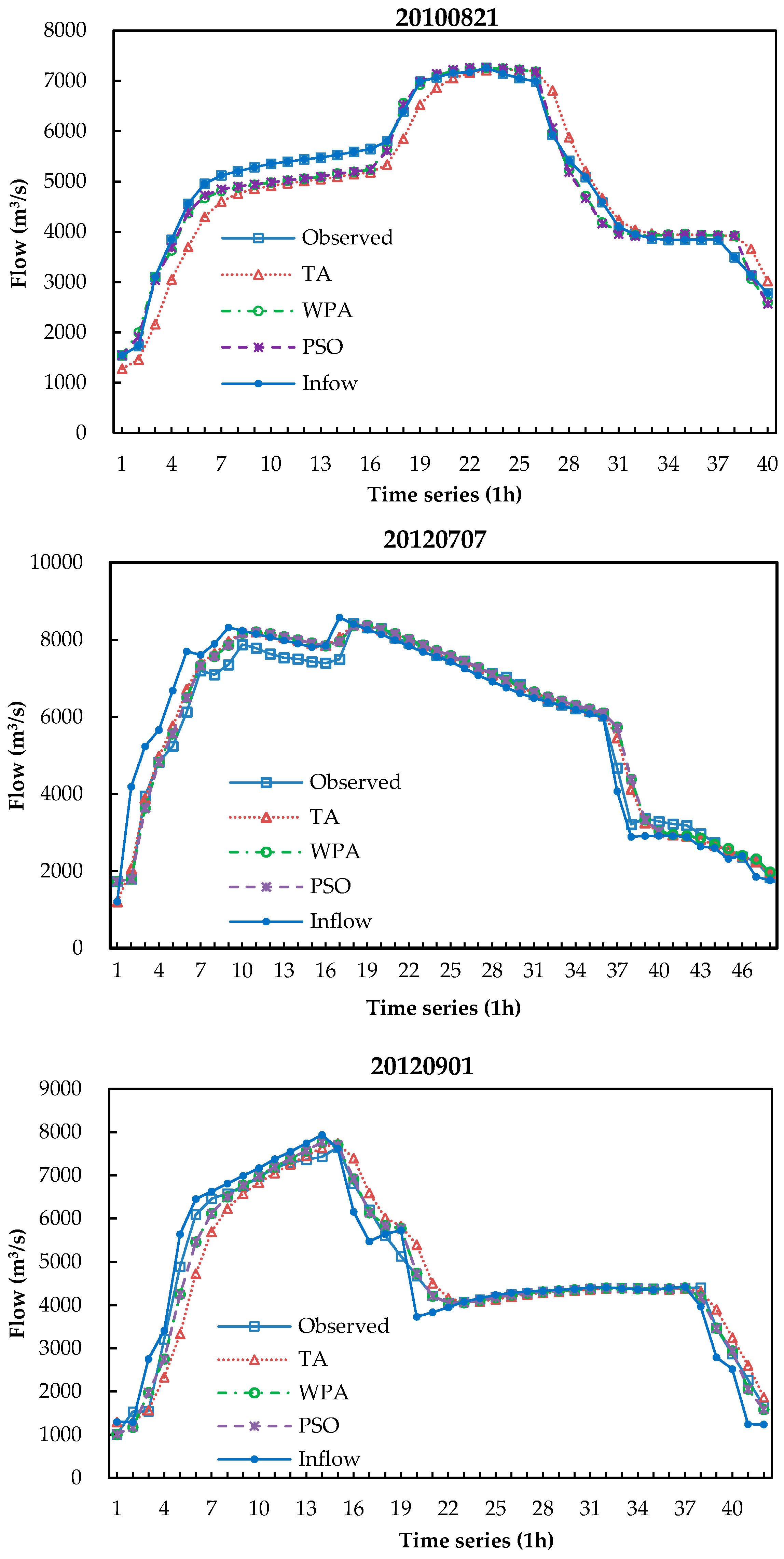
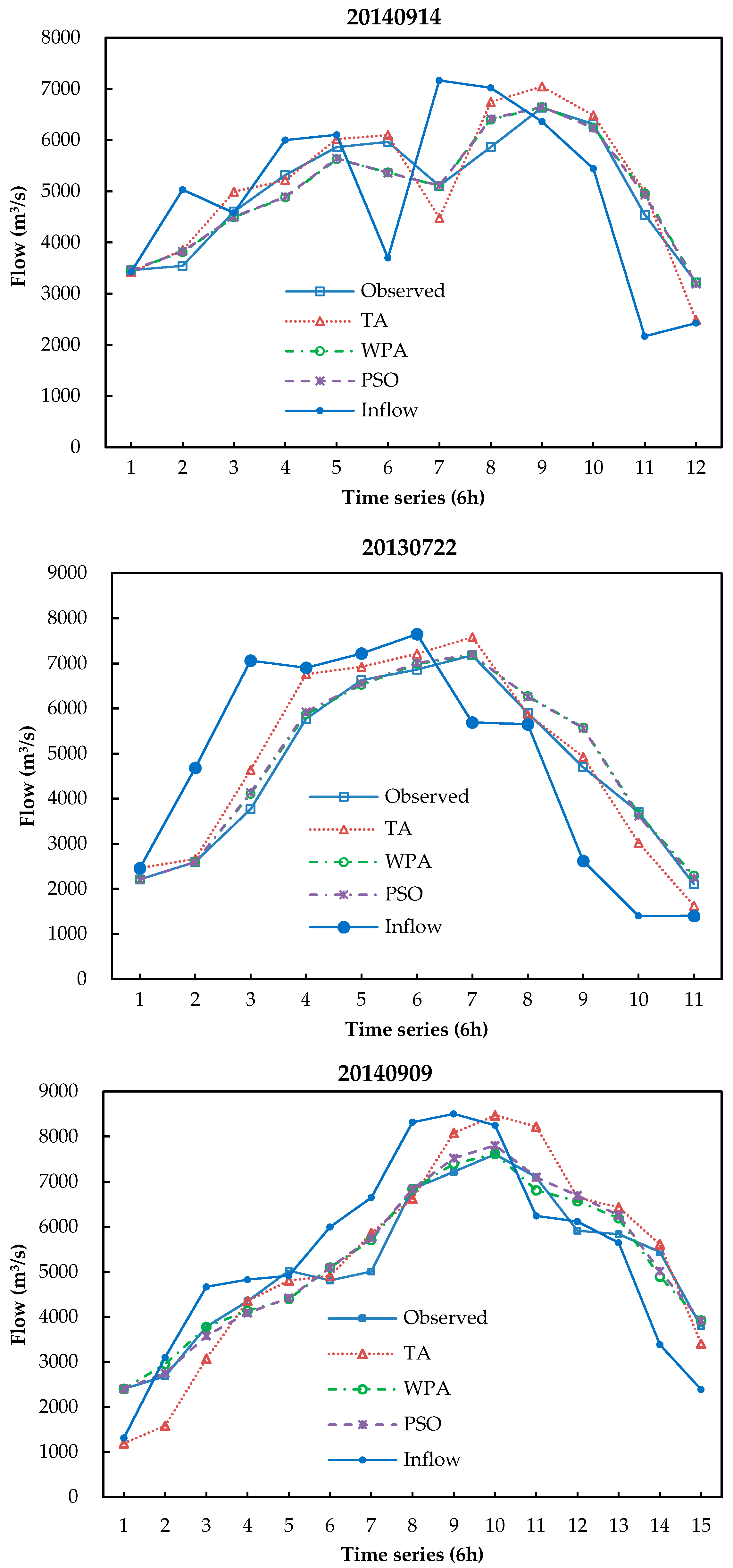
The comparison of the observed and simulation results of these three methods is presented in Figure 3 and Figure 4.

As shown in Figure 3 and Figure 4:

(1) No matter the length of the river, the simulation results of the WPA and PSO compared to those of the TA have a high fitting effect. It is embodied in the following aspects: The simulated peak values are the same as the observed ones, and the simulation process of the backwater segment is almost coincident with the observed process. However, the simulated values by the WPA and PSO in the rising water segment are different from the observed ones. Compared with the observed values, the deviation errors of the simulation values of the WPA are smaller than those of the PSO, and the deviation errors of the simulation values of the TA are the biggest.

(2) The fitting degree of the flood process in short reach is higher than that of the long river section by the WPA, PSO, and TA. Regardless of the length of the river, the error of the TA is the largest, and the WPA simulation deviation is slightly lower than that of the PSO.

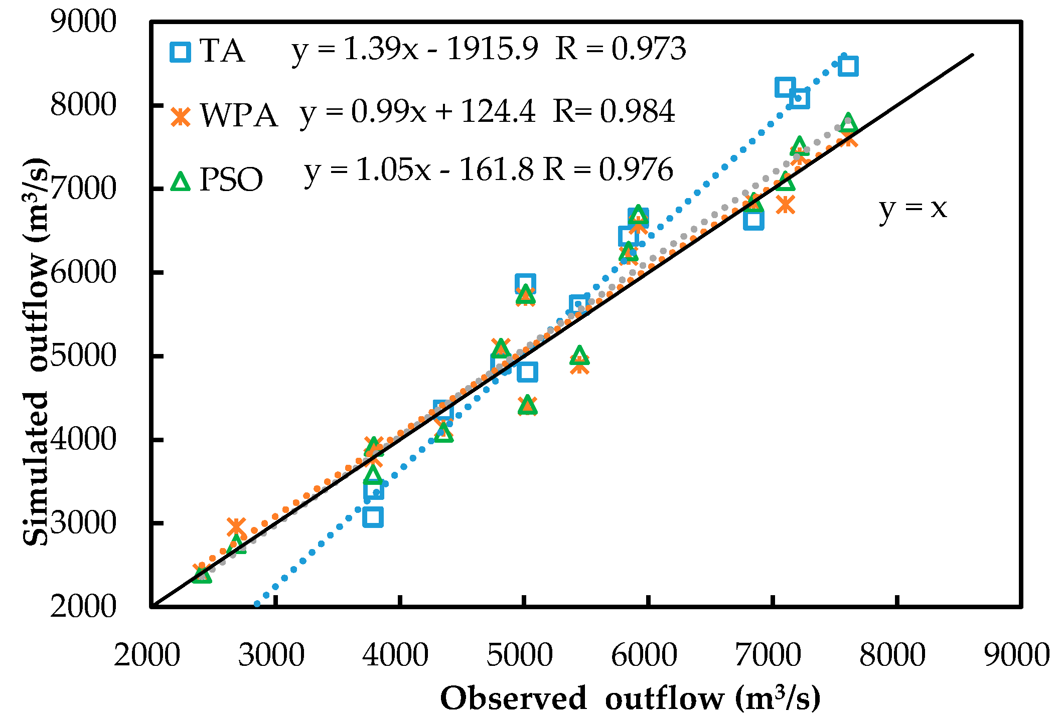
In order to visualize the fitting effect of the three methods, the 20140909 flood of Ankang Power Station to Shuhe Power Station was selected as an example (

Table 7. 20140909 flood simulation of Ankang Power Station to Shuhe Power Station.

Time	Inflow (m3/s)	Outflow (m3/s)				Relative Error (100%)
		Observed	TA	WPA	PSO	TA	WPA	PSO
0	1315	2405.47	1196.50	2405.47	2405.47	50.26%	0.00%	0.00%
6	3105	2682.43	1585.65	2956.10	2682.43	40.89%	10.20%	2.73%
12	4671	3783.79	3076.53	3784.10	3783.79	18.69%	0.01%	5.22%
18	4830	4351.65	4358.84	4141.88	4351.65	0.17%	4.82%	5.96%
24	4916	5026.62	4813.45	4400.83	5026.62	4.24%	12.45%	11.93%
30	5998	4813.56	4914.02	5102.37	4813.56	2.09%	6.00%	5.96%
36	6652	5010.76	5867.91	5709.84	5010.76	17.11%	13.95%	14.74%
42	8318	6846.56	6631.47	6836.78	6846.56	3.14%	0.14%	0.00%
48	8505	7217.19	8082.39	7395.13	7217.19	11.99%	2.47%	4.20%
54	8251	7607.34	8473.15	7616.87	7607.34	11.38%	0.13%	2.59%
60	6247	7101.53	8221.21	6816.21	7101.53	15.77%	4.02%	0.01%
66	6120	5917.64	6654.63	6574.14	5917.64	12.45%	11.09%	13.25%
72	5649	5839.00	6438.00	6196.58	5839.00	10.26%	6.12%	7.21%
78	3390	5446.03	5613.68	4897.68	5446.03	3.08%	10.07%	7.84%
84	2390	3789.75	3409.38	3925.44	3789.75	10.04%	3.58%	3.53%

), and the correlation diagram of observed and simulated flow are drawn in Figure 5.

As shown in Figure 5:

(1) The flooding process of the WPA simulation has 4 points falling on the line, and the trend line coefficient of WPA simulated flood process is 0.99, which is close to 1 compared to that of the PSO and TA, which indicates that the WPA has a high precision in the simulation of the whole flood process.

(2) The simulated flood peeks of the WPA fall in the straight line $y=x$, which indicates that the simulation value is equal to the observed. The peak values of the PSO and TA fall on the upper side of the line $y=x$, which indicates that the WPA has better simulation effect on peak value.

In order to further assess the precision of the WPA on the flood process and flood peak transmission time, the absolute deviation ($\delta$) of flood process, flood peak deviation, and flood peak transmission time error are selected as the evaluation indices.

Table 8. Analysis of Ankang hydropower station–Ankang city simulation results.

Floods	20100821			20120707			20120901
Method	TA	PSO	WPA	TA	PSO	WPA	TA	PSO	WPA
δ (m3/s)	13,960	7892	7865	11,404	10,606	10,607	197,269	5529	5528
Flood peak deviation (m3/s)	34.3	6.5	0.5	33	51.6	51.4	87.76	52.1	51.7
Flood peak time transmission error (h)	1	0	0	0	0	0	1	0	0

and

Table 9. Analysis of Ankang hydropower station–Shuhe hydropower station simulation results.

Floods	20130722			20140909			20140914
Method	TA	PSO	WPA	TA	PSO	WPA	TA	PSO	WPA
δ (m3/s)	4666	2221	2162	9141	4422	4278	4389	2697	2678
Flood peak deviation (m3/s)	402.0	19.5	0.3	865.8	197.1	9.5	409.0	15.0	8.6
Flood peak time transmission error (h)	0	0	0	0	0	0	0	0	0

show the indices values by the WPA, PAO, and TA of different floods.

As shown in Table 8 and Table 9:

(1) The WPA and PSO simulation results have a significant advantage over the results of the TA. Compared to that of the TA, the depreciation of absolute deviation cumulative value of flood process calculated by the WPA and PSO are 53% and 52%, respectively. The depreciation of absolute deviation of flood peak calculated by the WPA and PSO are 99% and 77% based on the 20140909 flood of Ankang power station–Shuhe hydropower station, respectively.

(2) The maximum deviations of the WPA, PSO, and TA are 9.5 m³/s, 197.1 m³/s and 865.8 m³/s, respectively. Moreover, the minimum deviations are 0.3 m³/s, 15 m³/s, and 402 m³/s, respectively, which indicate that the flood peak simulated by the WPA and PSO has obvious advantages over that of the TA. In the 20140909 flood simulation, flood peak deviations are 9.5 m³/s by the WPA and 197.1 m³/s by the PSO, respectively. Flood peak deviation simulated by the WPA is much smaller than that of the PSO, which indicates that the WPA can significantly improve peak forecast accuracy.

5. Conclusions

In this paper, a new multi-objective Muskingum model was established and solved by a new algorithm called the WPA, and its performance was verified by using the Ankang to Shuhe section of Hanjing River datasets. The following work has been done:

(1) After a brief literature review, a novel parameter estimation approach based on the WPA was proposed for parameter estimation of the nonlinear Muskingum flood, which considered two calibration objectives in the calibration procedure: (1) The weighted sum of absolute difference between the routed and observed outflows, and (2) the coefficient of determination between the routed and observed outflows.

(2) The proposed approach is compared to the other methods (TA, PSO) for an example case from the Hanjiang River, and the results demonstrate that the WPA can achieve a high degree of accuracy to estimate the parameters and results in accurate predictions of outflow.

(3) In this study, however, the parameters of WPA, such as the distance judgment factor and the step factor, have limited its application range. A possible reason is that different rivers have its applicable parameters. In future research, more floods in different rivers basins will be used to expand its range of applications.

References

- Kuriqi, A.; Ardiçlioglu, M.; Muceku, Y. Investigation of Seepage Effect on River Dike’s Stability under Steady State and Transient Conditions. Pollack Period. 2016, 11, 87–104. [Google Scholar] [CrossRef]
- Sajikumar, N.; Gyncy, I.; Sumam, K.S. Modelling of Nonlinear Muskingum Method using Control System Concept. Aquat. Procedia 2015, 4, 979–985. [Google Scholar] [CrossRef]
- Mccarthy, G. The unit hydrograph and flood routing. In Proceedings of the Conference of the North Atlantic Division, U.S. Engineer Department, New London, CT, USA, 24 June 1938; pp. 608–609. [Google Scholar]
- Luo, J.; Xie, J. Discussion of “Parameter Estimation for Nonlinear Muskingum Model Based on Immune Clonal Selection Algorithm”. J. Hydrol. Eng. 2010, 15, 391–392. [Google Scholar] [CrossRef]
- Xu, D.M.; Qiu, L.; Chen, S.Y. Estimation of Nonlinear Muskingum Model Parameter Using Differential Evolution. J. Hydrol. Eng. 2012, 17, 348–353. [Google Scholar] [CrossRef]
- Gill, M.A. Flood routing by the Muskingum method. J. Hydrol. 1978, 36, 353–363. [Google Scholar] [CrossRef]
- Kuriqi, A.; Ardiçlioǧlu, M. Investigation of hydraulic regime at middle part of the Loire River in context of floods and low flow events. Pollack Period. 2018, 13, 145–156. [Google Scholar] [CrossRef]
- Mohon, S. Parameter Estimation of Nonlinear Muskingum Models Using Genetic Algorithm. J. Hydraul. Eng. 1997, 123, 137–142. [Google Scholar] [CrossRef]
- Chen, J.; Yang, X. Optimal parameter estimation for Muskingum model based on Gray-encoded accelerating genetic algorithm. Commun. Nonlinear Sci. Numer. Simul. 2007, 12, 849–858. [Google Scholar] [CrossRef]
- Chu, H.J.; Chang, L.C. Applying Particle Swarm Optimization to Parameter Estimation of the Nonlinear Muskingum Model. J. Hydrol. Eng. 2009, 14, 1024–1027. [Google Scholar] [CrossRef]
- Barati, R. Discussion of Parameter Estimation of the Nonlinear Muskingum Model Using Parameter-Setting-Free Harmony Search. J. Hydrol. Eng. 2011, 17, 1414–1416. [Google Scholar] [CrossRef]
- Zhang, H.; Li, Z.; Kan, G.; Yao, C. Muskingum parameter estimation method based on SCE-UA algorithm and its realization in programming. J. Hydraul. Eng. 2013, 32, 43–47. (In Chinese) [Google Scholar]
- Niazkar, M.; Afzali, S.H. Application of New Hybrid Optimization Technique for Parameter Estimation of New Improved Version of Muskingum Model. Water Resour. Manag. 2016, 30, 4713–4730. [Google Scholar] [CrossRef]
- Ouyang, A.; Liu, L.B.; Sheng, Z.; Wu, F. A Class of Parameter Estimation Methods for Nonlinear Muskingum Model Using Hybrid Invasive Weed Optimization Algorithm. Math. Probl. Eng. 2015, 2015, 573894. [Google Scholar] [CrossRef]
- Gupta, H.V.; Sorooshian, S.; Yapo, P.O. Toward improved calibration of hydrologic models: Multiple and noncommensurable measures of information. Water Resour. Res. 1998, 34, 3663–3674. [Google Scholar] [CrossRef]
- Bekele, E.G.; Nicklow, J.W. Multi-objective automatic calibration of SWAT using NSGA-II. J. Hydrol. 2007, 341, 165–176. [Google Scholar] [CrossRef]
- Zhang, S.; Kang, L.; Zhou, L.; Guo, X. A new modified nonlinear Muskingum model and its parameter estimation using the adaptive genetic algorithm. Hydrol. Res. 2017, 48, 17–27. [Google Scholar] [CrossRef]
- Vatankhah, A.R. Nonlinear Muskingum model with inflow-based exponent. Water Manag. 2016, 170, 66–80. [Google Scholar] [CrossRef]
- Moghaddam, A.; Behmanesh, J.; Farsijani, A. Parameters Estimation for the New Four-Parameter Nonlinear Muskingum Model Using the Particle Swarm Optimization. Water Resour. Manag. 2016, 30, 2143–2160. [Google Scholar] [CrossRef]
- Luo, J.; Zhang, X.; Zhang, X. Multi-Objective Calibration of Nonlinear Muskingum Model Using Non-Dominated Sorting Genetic Algorithm-II. Int. Conf. Appl. Math. Simul. Model. 2016. [Google Scholar] [CrossRef] [Green Version]
- Easa, S.M. Multi-criteria optimization of the Muskingum flood model: A new approach. Water Manag. 2015, 168, 220–231. [Google Scholar] [CrossRef]
- Bao, W.M.; Zhang, J.Y. Hydrologic Forecasting, 4th ed.; China Water and Power Press: Beijing, China, 2009; pp. 3–93. (In Chinese) [Google Scholar]
- Liu, C.Y.; Yan, X.H.; Wu, H. The Wolf Colony Algorithm and Its Application. Chin. J. Electron. 2011, 20, 212–216. (In Chinese) [Google Scholar]
- Karahan, H.; Gurarslan, G.; Zong, W.G. Parameter Estimation of the Nonlinear Muskingum Flood Routing Model Using a Hybrid Harmony Search Algorithm. J. Hydrol. Eng. 2013, 18, 352–360. [Google Scholar] [CrossRef]
- Easa, S.M. New and improved four-parameter non-linear Muskingum model. Water Manag. 2015, 167, 288–298. [Google Scholar] [CrossRef]
- Zhang, G.; Xie, T.; Zhang, L.; Hua, X.; Wu, C.; Chen, X.; Li, F.; Zhao, B. “In-Process Type” Dynamic Muskingum Model Parameter Estimation Method. Water 2017, 9, 849. [Google Scholar] [CrossRef]
- Song, X.M.; Kong, F.Z.; Zhu, Z.X. Application of Muskingum routing method with variable parameters in ungauged basin. Water Sci. Eng. 2011, 4, 1–12. [Google Scholar] [CrossRef]
- Franchini, M.; Bernini, A.; Barbetta, S.; Moramarco, T. Forecasting discharges at the downstream end of a river reach through two simple Muskingum based procedures. J. Hydrol. 2011, 399, 335–352. [Google Scholar] [CrossRef]
- Wu, H.S.; Zhang, F.M.; Wu, L. New swarm intelligence algorithm-wolf pack algorithm. Syst. Eng. Electron. 2013, 35, 2430–2438. [Google Scholar] [CrossRef]
- Lai, L.H. Research on gyroscope random drift modeling based on ARMA model and wolf pack algorithm. Transducer Microsyst. Technol. 2016, 35, 56–58. (In Chinese) [Google Scholar]
- Wang, J.; Jiao, Y. Improvement of wolf pack search algorithm and its application to optimal operation of reservoirs. Eng. J. Wuhan Univ. 2017, 50, 161–167. (In Chinese) [Google Scholar]
Figure 1.
Map of the Hanjiang River and the location of major reservoirs.
Figure 2.
Flow chart of parameter estimation.
Figure 3.
Simulation results of different floods in Reach 1.
Figure 4.
Simulation results of different floods in Reach 2.
Figure 5.
Correlation of observed and simulation data.