Artificial Neural Networks for Predicting the Water Retention Curve of Sicilian Agricultural Soils

Abstract

Modeling soil-water regime and solute transport in the vadose zone is strategic for estimating agricultural productivity and optimizing irrigation water management. Direct measurements of soil hydraulic properties, i.e., the water retention curve and the hydraulic conductivity function, are often expensive and time-consuming, and represent a major obstacle to the application of simulation models. As a result, there is a great interest in developing pedotransfer functions (PTFs) that predict the soil hydraulic properties from more easily measured and/or routinely surveyed soil data, such as particle size distribution, bulk density (ρ_b), and soil organic carbon content (OC). In this study, application of PTFs was carried out for 359 Sicilian soils by implementing five different artificial neural networks (ANNs) to estimate the parameter of the van Genuchten (vG) model for water retention curves. The raw data used to train the ANNs were soil texture, ρ_b, OC, and porosity. The ANNs were evaluated in their ability to predict both the vG parameters, on the basis of the normalized root-mean-square errors (NRMSE) and normalized mean absolute errors (NMAE), and the water retention data. The Akaike’s information criterion (AIC) test was also used to assess the most efficient network. Results confirmed the high predictive performance of ANNs with four input parameters (clay, sand, and silt fractions, and OC) in simulating soil water retention data, with a prediction accuracy characterized by MAE = 0.026 and RMSE = 0.069. The AIC efficiency criterion indicated that the most efficient ANN model was trained with a relatively low number of input nodes.

1. Introduction

Soil hydraulic properties are important for simulating water availability and transmission in soils. An important hydraulic property of the soil is the water retention capacity, which affects productivity and soil management. Knowledge of water retention capacity and the effects of land use on this property is critical to efficient soil and water management and to estimate irrigation water supply, which may be affected by changes in the use of soil [1].

The availability of easily accessible and representative soil hydraulic properties is generally a major obstacle to understanding the dynamics of water and solutes in the unsaturated soil [1] and the application of simulation models to prevent and control deterioration of soil due to intensive agricultural activities.

In agricultural contexts, the management of irrigation and drainage and the related plant growth and activity require crucial information on soil properties, such as the soil water retention curve and the unsaturated hydraulic conductivity function [2], which in turn allow modeling of water flow in the vadose zone. Due to their high spatial variability, determination of these properties requires a larger number of soil samples, thus implying expensive and time-consuming field and laboratory analyses [3] that make the direct measurements of soil hydraulic properties quite impractical.

An attractive alternative to the direct measurement of hydraulic properties is their estimation by pedotransfer functions (PTFs). PTFs have been adopted for decades as tools to estimate soil hydraulic properties starting from more easily available soil characteristics (i.e., particle size distribution, soil porosity, organic matter, and bulk density) [4]. Most of the PTFs reported in literature pertain to the estimation of soil water retention points, such as field capacity, permanent wilting point, and plant available water capacity. Parametric PTFs, instead, offer a continuous and smooth representation of the soil water retention curve, which is preferred for modeling purposes. Among the various expressions proposed in the literature to represent the soil water retention curve, the van Genuchten equation (vG) [5] is currently the most widely used [6] and PTFs for predicting its parameters were built, among others, by the authors of References [7,8,9,10,11]. An advantage of the vG equation over other expressions (e.g., References [12,13]) is that the slope of the soil water retention curve is continuous, thus preventing convergence problems in numerical saturated–unsaturated flow problems [14].

Studies in PTF enhancement focus on the development of better functions to estimate soil hydraulic properties for different geographical areas or soil types and determination of the most important basic soil properties as input [15]. Many comparisons of PTF_s have been made in respect to different data sets used, different mathematical procedures (regression versus artificial neural network models), and different input parameters.

When a large database of soil properties is available, artificial neural networks (ANNs) are frequently used to support the hydrological modeling [16]. The ANN has a “black box” nature able to simulate the human brain, which memorizes, learns, associates, and comprises the complex interactions (networks) between data (input, neurons of the hidden layers, and output) [17]. It does not imply any pre-existing knowledge of the relationships between input and output. This means that ANNs require no a priori model concept (they are commonly called black boxes) and they are able to extract the maximum amount of information from the data. Several attempts were carried out to adopt ANNs to predict soil hydraulic properties. For example, Reference [16] developed an ANN capable of predicting the soil water content at any matric potential, without using specific equations or parameterizations; the research proposed by Reference [1] presented two different PTF models trained with fitted water content data; the study of Reference [18] used ANNs to predict the plant available water capacity; and Reference [14] used PTFs and ANNs to predict the soil water retention and the available water of sandy soils. In their research, some of these authors proved how useful it is to train an ANN with a wide range of soil matric potentials to account for most of the variations that are likely to be encountered in the soil, rather than having water retention data collected in a limited range of water potential [14,18].

Notable review articles dwelling on PTF development and its applications include References [11,19]. Reference [11] discussed the accuracy and reliability of PTFs and emphasized that the future developments in PTFs would come from better data-mining tools like neural networks. Reference [20], in their review, evidenced that empirical PTFs (such as that developed by Reference [21]), require a large set of prediction equations to determine the water retention curve. Most recent PTFs reported in the literature used a neural network approach. An advantage of artificial neural networks (ANNs) is their ability to mimic the behavior of complex systems by varying the strength of influence of network components, as well as the structures of interconnections among components. An ANN is simply a sophisticated regression, which has a network of many simple elements (or neurons). ANNs require no a priori model concept, and extract the maximum amount of information from the data.

In the agricultural context of Sicily (southern Italy), where very limited studies on soil physical and hydraulic properties are available in sufficient detail to support irrigation management, a project was initiated to bring together the existing hydraulic datasets collected by the Agricultural Departments of the Universities of Palermo and Catania into a unique database with the aim to train ANNs specifically developed for Sicily. In this research, funded by the Sicilian Region, innovative methodologies for the rapid evaluation of the physical soil quality on a territorial scale were developed. In particular, the applicability of the simplified falling head (SFH) technique and of the Beerkan estimation of soil transfer parameters (BEST) method was evaluated, aimed at surveying the hydraulic properties of the soil [22,23,24].

Starting from the outcomes of the abovementioned project, the main objectives of the present study were (i) to evaluate the reliability of the artificial neural network approach (ANN), implemented with a large and variable database of soil characteristics, when estimating the vG model parameters, and (ii) to identify the ANN structure that guarantees the best prediction performance for the soil water retention curve using evaluation criteria.

2. Materials and Methods

2.1. Soil Samples

Data collected in a total of 359 soil horizons were used for the purpose of the study. The database contains soil data from 21 sites of the Sicilian territory (insular Italy), covering a wide range of soil types and characteristics [22,23,24]. In particular, the following data were available for each sampling point: clay (Cl), silt (Si), and sand (Sa) fractions, dry bulk density (ρ_b), geometric mean particle diameter (d_g), organic carbon content (OC), porosity (φ), and volumetric soil water content (θ), determined during a drying sequence of at least eleven matric heads (h) in the range from −0.01 to 150 m. Fractions of Cl, Si, and Sa were determined according to the United States Department of Agriculture (USDA) standard for particle size distribution conducted using the hydrometer method for particles having diameters d < 74 mm and by sieving for particles with 74 ≤ d ≤ 2000 [25]. The texture triangle in Figure 1 shows that all USDA classes were included in the considered database. For each investigated site,

Table 1. Mean values and standard deviations of the fractions of clay (Cl), silt (Si), and sand (Sa), geometric mean particle diameter (d_g), dry soil bulk density (ρ_b), organic carbon content (OC), and porosity (φ) for the investigated Sicilian soils; n is the number of sampled soils at each site.

Site	n	Clay (%)	Silt (%)	Sand (%)	dg (mm)	OC (g·kg−1)	ρb (Mg·m−3)	φ
Palermo	3	18.0 (±1.7)	28.6 (±2.5)	53.4 (±3.5)	0.10 (±0.02)	3.4 (±1.19)	1.1.2 (±0.04)	0.58 (±0.01)
Bulgherano	32	16.4 (±3.8)	27.1 (±3.9)	56.5 (±4.1)	0.13 (±0.03)	2.1 (±0.52)	1.25 (±0.10)	0.53 (±0.04)
Caccamo	1	7.4	18.0	74.6	0.02	1.51	1.25	0.53
Castelvetrano	5	35.3 (±7.9)	24.0 (±4.6)	40.7 (±4.0)	0.04 (±0.02)	2.0 (±0.50)	1.31 (±0.07)	0.51 (±0.03)
Comiso	1	28.2	46.5	25.3	0.03	2.8	1.09	0.59
Corleone	6	41.2 (±19.1)	32.4 (±2.5)	26.4 (±21.1)	0.04 (±0.06)	2.2 (±0.67)	1.07 (±0.17)	0.60 (±0.06)
Etna	1	0.5	9.7	89.9	0.70	1.86	1.37	0.48
Dirillo	85	20.6 (±11.1)	33.6 (±15.9)	45.7 (±25.7)	0.15 (±0.17)	1.1 (±0.73)	1.40 (±0.16)	0.47 (±0.06)
Menfi	82	(±11.4)	(±10.1)	47.0 (±18.4)	0.12 (±0.10)	1.5 (±0.21)	1.26 (±0.14)	0.52 (±0.05)
Mineo	2	21.8	(±2.3)	32.5 (±6.6)	0.04 (±0.02)	1.5 (±0.66)	1.26 (±0.03)	0.52 (±0.01)
Monreale	1	5.4	22.7	71.9	0.31	0.3	1.26	0.53
Palazzelli	32	10.5 (±3.8)	(±5.8)	69.7 (±7.6)	0.26 (±0.09)	1.2 (±0.27)	1.25 (±0.08)	0.53 (±0.03)
Pettineo	1	24.9	34.2	40.9	0.05	4.6	1.14	0.57
Pollina	2	24.8 (±4.17)	(±8.9)	33.8 (±13.1)	0.04 (±0.03)	3.6 (±0.18)	1.15 (±0.02)	0.57 (±0.01)
Ramacca	2	29.7 (±4.4)	(±2.7)	35.5 (±7.1)	0.04 (±0.01)	0.7 (±0.46)	1.32 (±0.00)	0.50 (±0.00)
Rapitalà	2	28.3 (±11.7)	(±11.4)	34.8 (±23.1)	0.05 (±0.05)	1.6 (±0.22)	1.30 (±0.10)	0.51 (±0.04)
Resuttano	6	51.1 (±17.5)	(±13.1)	7.1 (±5.9)	0.01 (±0.01)	1.6 (±1.17)	1.30 (±0.15)	0.51 (±0.06)
Santa Ninfa	52	20.5 (±18.4)	(±16.0)	21.6 (±9.9)	0.04 (±0.02)	3.4 (±1.38)	1.13 (±0.09)	0.57 (±0.03)
San Michele	40	46.7 (±6.6)	(±6.2)	36.3 (±9.0)	0.02 (±0.01)	2.5 (±0.49)	1.27 (±0.08)	0.52 (±0.03)
Sparacia	2	17.2 (±7.8)	(±2.0)	62.3 (±5.7)	0.15 (±0.07)	0.5 (±0.0)	1.40 (±0.11)	0.47 (±0.04)
Ventimiglia	1	36.3	29.8	33.9	0.03	1.3	1.25	0.53
All	359	23.9	31.3	44.8	0.11	2	1.25	0.53

summarizes the descriptive statistics of the selected soil physical properties.

The geometric mean particle diameter d_g (mm) was calculated according to Reference [26]:

$$d_g=\exp \left\{\left(\mathrm{Cl}·\ln \left({\mathrm{M}}_{\mathrm{cl}}\right)+\mathrm{Si}·\ln \left({\mathrm{M}}_{\mathrm{si}}\right)+\mathrm{Sa}·\ln \left({\mathrm{M}}_{\mathrm{sa}}\right)\right)\right\}$$

(1)

where Cl, Si, and Sa are the clay, silt, and sand fractions of soil (g·g⁻¹), respectively, and M_cl, M_si, and M_sa are the mean diameters of clay, silt, and sand, respectively (M_cl = 0.001 mm; M_si = 0.026 mm; M_sa = 1.025 mm).

The organic carbon content, OC (%), was determined using the Walkley–Black method [27]. Undisturbed soil cores were used to determine the soil bulk density (ρ_b, Mg·m⁻³), and porosity (φ) was calculated assuming a value of the soil particle density equal to 2.65 Mg·m⁻³.

Water retention data were determined on undisturbed soil samples using a hanging water column apparatus [24] or a sandbox apparatus [22] for h values ranging from −0.05 to −1.5 m. A pressure plate apparatus with repacked soil samples was used to determine θ values corresponding to h in the range from −3 to −150 m. To account for the different number of θ(h) points among samples and different applied equilibrium h values, the water retention model proposed by van Genuchten [5] was fitted to experimental data:

$$\theta \left(h\right)={\theta }_r+\frac{{\theta }_s-{\theta }_r}{{\left(1+{\left|\alpha h\right|}^n\right)}^m}$$

(2)

where θ (cm³·cm⁻³) is the water content at matric potential h (cm), θ_s and θ_r are the saturated and residual water contents (cm³·cm⁻³), respectively, n (-) is the curve shape factor which controls the steepness of the S-shaped retention curve, m (-) is an empirical shape factor related to n by m = 1 − (1/n), and α (cm⁻¹) is an empirical scale parameter related to the inverse of the air entry suction. Fitting of Equation (2) to experimental data was carried out using the RETC software [28]. Figure 2 shows, for each site, the mean fitted water retention curve. The mean value of root-mean-square error (RMSE) ranged from 0.005 to 0.047, with an average value for Sicily equal to 0.014.

For each soil, water contents corresponding to eleven matric potentials (h = −1, −2.5, −10, −31.6, −63.1, −100, −300, −1000, −3000, −6000, and −15,000 cm) were, thus, calculated from the fitted Equation (2) and assumed as measured reference values for the evaluation of ANN performance.

2.2. Artificial Neural Networks (ANNs)

The generalized feed-forward (GFF) neural network was identified for modeling soil water retention of the Sicilian soil database. This ANN model is a generalization of the multi-layer perceptron (MLP), that is often used for modeling physical processes [29]. In an MLP, any neuron of a hidden layer receives input from all neurons of the previous layer and sends its output to all neurons of the following layer. Unlike MLP, GFF has connections between neurons of non-adjacent layers. These types of networks are called “feed-forward”, because the signals propagate only from the input to the output. Furthermore, they are usually trained with supervised learning; this means that they are trained with a subset of measured input and output pairs.

The ANN architecture proposed in this study was composed of one input layer, two hidden layers with 15 neurons each, and one output layer (Figure 3). The number of neurons in the input layer varied from three to four in relation to the chosen set of input parameters. Specifically, five combinations of inputs were investigated, as reported in

Table 2. Combination of inputs in the developed artificial neural networks (ANNs).

Network	Input Data 1
ANN1	Cl, Si, dg, φ
ANN2	Cl, Sa, ρb
ANN3	Cl, Sa, OC
ANN4	Cl, Sa, Si, OC
ANN5	Cl, Sa, OC, ρb

¹ Clay (Cl), silt (Si), sand (Sa) percentages; geometric mean particle diameter (d_g), dry soil bulk density (ρ_b), organic carbon content (OC), and porosity (φ).

.

The number of neurons in the output layer was four in all the developed ANNs, corresponding to the number of estimated parameters—θ_s, θ_r, α, and n. The transfer function was the hyperbolic tangent for all the layers.

The ANN training phase was performed using a backpropagation algorithm with a momentum term that improves the convergence of the network by changing weights along an error gradient. Specifically, the learning rates adopted for the connections of the input layer, the first hidden layer, and the second hidden layer were 0.1, 0.001, and 0.1, respectively. The momentum factor was 0.6 for all layers. The weights were updated online; they were modified after the presentation of each input pattern.

As the training of an ANN is heavily influenced by the initial values of the weights, several training cycles are generally carried out starting with different sets of random weight values. In this study, the learning of the networks was performed through five cycles of training. At the end of learning, the weights obtained by the cycle that provided the minimum mean squared error (MSE) were chosen. The maximum number of epochs for each training cycle was 50,000. The ending criterion adopted for the training process was cross-validation. This technique consists of checking the network performance at each iteration with a set of data not used for training. The training stops when the MSE calculated for the crossing data does not improve further after an established number of epochs. The number of epochs chosen to stop each training cycle without improvements in the performance of the cross-validation set was 2000, as it was observed [29] that it is sufficiently high to ensure that there is no further possibility of refining the results. The ability of the network to generalize was tested using a new set of data, which was different from that used for training and cross-validation. In particular, the 359 elements of the dataset were randomly ordered and divided as follows: 215 for training, 54 for cross-validation, and 90 for testing. The ANNs were implemented using the Neurosolutions 7 software (NeuroDimension, Inc., Gainesville, FL, USA).

Mean, minimum, and maximum absolute errors (MAE, Min AE, and Max AE), normalized mean absolute error (NMAE), root-mean-square error (RMSE), normalized root-mean-square error (NRMSE), and correlation coefficient (r) (

Table 3. Statistical indicators used to evaluate reliability of ANN modeling. MAE—mean absolute error; NMAE—normalized MAE; RMSE—root-mean-square error; NRMSE—normalized RMSE.

$MAE=\frac{{{\displaystyle \sum }}_{i=1}^n\left|y_i-x_i\right|}{n}$

$NMAE=\frac{MAE}{\overline{y}}$

$RMSE=\sqrt{\frac{{{\displaystyle \sum }}_{i=1}^n{\left(y_i-x_i\right)}^2}{n}}$

$NRMSE=\frac{RMSE}{\overline{y}}$

$r=\frac{{{\displaystyle \sum }}_{i=1}^n\left(x_i-\overline{x}\right)\left(y_i-\overline{y}\right)}{\sqrt{{{\displaystyle \sum }}_{i=1}^n{\left(x_i-\overline{x}\right)}^2\sqrt{{{\displaystyle \sum }}_{i=1}^n{\left(y_i-\overline{y}\right)}^2}}}$

$\overline{x}=\frac{{{\displaystyle \sum }}_{i=1}^n{x}_i}{n} \overline{y}=\frac{{{\displaystyle \sum }}_{i=1}^n{y}_i}{n}$

n is the sample size, y_i is the observed value, x_i is the predicted value.

) were used to assess the reliability in modeling the vG parameters. The MAE value is a measure of the mean error between estimated and measured values. The value of RMSE determines how well the network output fits the measured output. Both MAE and RMSE cannot be used to compare scores across variables with different numerical ranges. The NMAE and NRMSE statistics were used for this purpose, and they can be regarded as a performance ratio between the output values obtained with the ANN and the simple mean of the desired values. The means of NRMSE and NMAE obtained for θ_s, θ_r, α, and n were also calculated for each ANN, in order to compare the overall performance of each ANN in the simulation of the vG parameters. Estimated θ(h) values were calculated at the selected eleven matric potentials from Equation (2) with parameters θ_s, θ_r, α, and n obtained by the ANNs. The performance in simulating water retention was evaluated by means of MAE, RMSE, and determination coefficient (r²).

Parameters of vG are strongly interdependent [6]; thus, small errors in estimated parameters may result in large errors in water retention data predictions. To exclude the influence of the soil water retention curve parameterization on the results of ANNs, estimated θ(h) values at the selected eleven matric potentials were compared with the corresponding measured values. The performance in simulating water retention data was evaluated by means of MAE, RMSE, and determination coefficient (r²).

Because there are no general rules for selecting the number of hidden units in the ANN, and the larger number of hidden units implies more parameters to be estimated, in this study, Akaike’s information criterion (AIC) [30] was used to compare the different networks (Table 2) in order to evaluate of the most efficient ANN among the five listed in Table 2 [31]. Several studies in the literature showed the robustness of AIC in ANN selection for simulating hydrological processes [32,33,34]. For each network, the AIC value can be calculated by

$$AIC=n·\ln \left(\frac{RSS}{n}\right)+2·K\mathrm{if}n/K\ge 40$$

(3)

$$AIC=n·\ln \left(\frac{RSS}{n}\right)+2·K+\frac{2·K·\left(K+1\right)}{n-K-1}\mathrm{if} n/K<40$$

(4)

where n is the number of observations, K is the number of free parameters, and RSS is the residual sum of square. Lower AIC values correspond to higher network efficiency. When the AIC test is applied to an ANN, K is the number of the weights. Therefore, K = 481 for ANN1, ANN4, and ANN5, while K = 447 for ANN2 and ANN3. The AIC test was applied either to the difference between measured and estimated θ_s, θ_r, α, and n values or the difference between measured and estimated θ(h) values.

3. Results

The statistical indicators used to evaluate ANN performance are reported in

Table 4. Statistical indicators of ANN performance in modeling the test set.

ANNs	Performance	θr	θs	α	N
ANN1	RMSE	0.0679	0.0660	0.0973	0.2135
	NRMSE	0.2751	0.1135	0.0692	0.1277
	MAE	0.0571	0.0523	0.0596	0.1607
	NMAE	0.2314	0.0899	0.0424	0.0962
	Min AE	0.0039	0.0030	0.0021	0.0012
	Max AE	0.1710	0.1984	0.4797	0.7833
	r	0.2762	0.6612	0.2926	0.6944
ANN2	RMSE	0.0671	0.0677	0.0957	0.2113
	NRMSE	0.2718	0.1164	0.0681	0.1264
	MAE	0.0571	0.0533	0.0582	0.1581
	NMAE	0.2314	0.0917	0.0414	0.0946
	Min AE	0.0047	0.0004	0.0007	0.0016
	Max AE	0.1673	0.1953	0.4817	0.7828
	r	0.2927	0.6402	0.2766	0.7003
ANN3	RMSE	0.0650	0.0701	0.0967	0.2238
	NRMSE	0.2635	0.1206	0.0688	0.1339
	MAE	0.0555	0.0562	0.0574	0.1634
	NMAE	0.2248	0.0966	0.0408	0.0978
	Min AE	0.0024	10−5	0.0015	0.0019
	Max AE	0.1845	0.2339	0.4873	0.8500
	r	0.3789	0.6109	0.1586	0.6574
ANN4	RMSE	0.0610	0.0681	0.0972	0.2197
	NRMSE	0.2470	0.1172	0.0691	0.1315
	MAE	0.0500	0.0554	0.0556	0.1560
	NMAE	0.2025	0.0952	0.0396	0.0933
	Min AE	0.0018	0.0011	0.0003	0.0029
	Max AE	0.1764	0.2149	0.4908	0.8782
	r	0.5004	0.6400	0.1673	0.6734
ANN5	RMSE	0.0657	0.0641	0.1001	0.2120
	NRMSE	0.2663	0.1102	0.0712	0.1268
	MAE	0.0552	0.0515	0.0611	0.1567
	NMAE	0.2236	0.0885	0.0434	0.0937
	Min AE	0.0013	0.0013	0.0003	0.0004
	Max AE	0.1788	0.1856	0.4666	0.7842
	r	0.3764	0.6887	0.2318	0.6992

. The analysis of the indicators showed that all the ANNs were efficient in estimating parameter α with NRMSE and NMAE values in the range of 0.068–0.071 and 0.039–0.043, respectively. Higher values were reached for θ_s, with NRMSE values of 0.11–0.12 and NMAE values of 0.088–0.096, and for n, with NRMSE values of 0.1264–0.1339 and NMAE values of 0.093–0.097. The lowest performance was obtained for θ_r with NRMSE and NMAE values in the range 0.24–0.27 and 0.20–0.23, respectively.

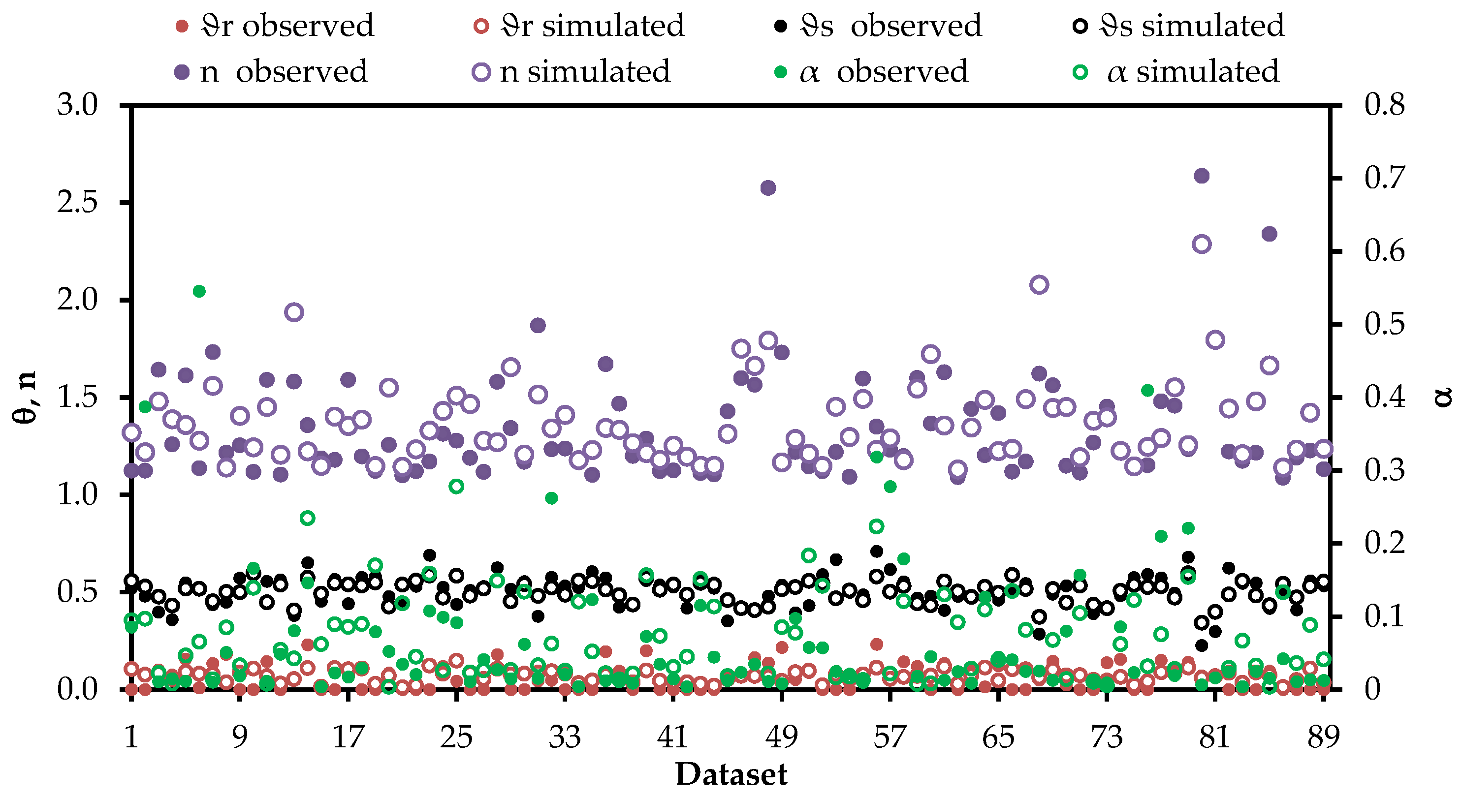
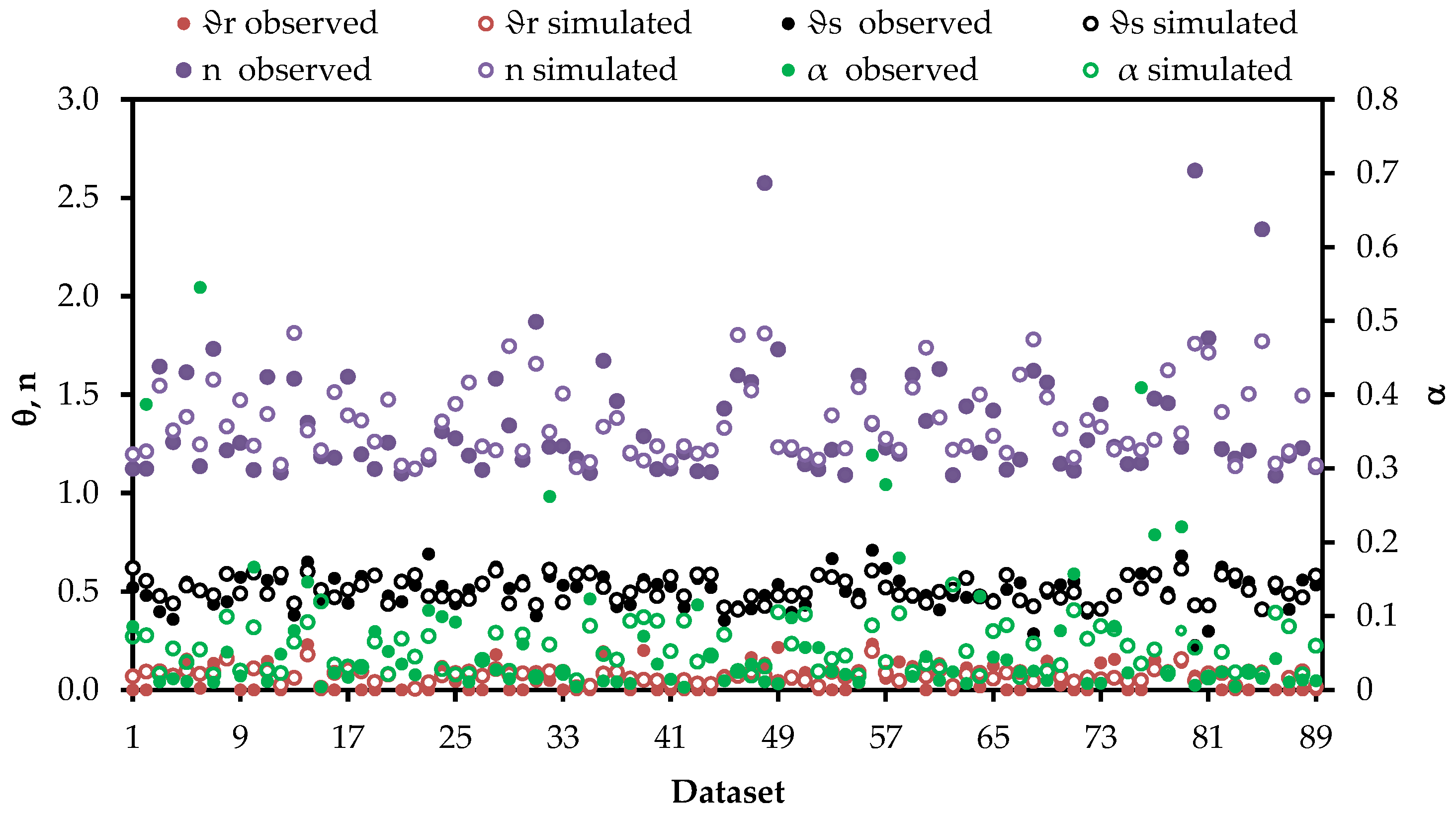
The coefficient of correlation (r) had the highest values (r = 0.61–0.70) for θ_s and n, and the lowest values (r = 0.16–0.50) for θ_r and α. In this regard, it can be shown that r is oversensitive to extreme values (outliers), which characterized θ_r and α much more than θ_s and n, both having a narrower range of variation. As an example, the trends of the observed and simulated vG parameters are reported in Figure 4 for ANN1 and in Figure 5 for ANN4. Mean values of NRMSE and NMAE obtained for θ_r, θ_s, α, and n were also calculated for each ANN in order to compare the overall performance in the simulation of the vG parameters. Although the results were very similar, it can be noted that the lowest values were achieved by ANN4 (NRMSE = 0.1412 and NMAE = 0.1077), while the highest ones were obtained by ANN3 (NRMSE = 0.1467 and NMAE = 0.1150). Intermediate values were obtained by ANN5 (NRMSE = 0.1436 and NMAE = 0.1123), ANN2 (NRMSE = 0.1457 and NMAE = 0.1148) and ANN1 (NRMSE = 0.1464 and NMAE = 0.1150).

Table 5. Statistical indicators of ANN performance in simulating water retention.

Network	MAE	RMSE	r2
ANN1	0.030	0.074	0.75
ANN2	0.032	0.076	0.74
ANN3	0.032	0.089	0.65
ANN4	0.026	0.069	0.79
ANN5	0.016	0.074	0.72

reports the MAE and RMSE values for the estimated soil water retention data obtained with the considered ANNs. The calculations refer to the test dataset that comprises 90 soils. It is worth noting that ANNs that made use of four input data generally performed better than those that used three input data. Specifically, the minimum MAE was obtained by ANN5, while ANN4 had the minimum RMSE. Less satisfactory results were obtained by ANN1, whereas the highest values of both MAE and RMSE were obtained with ANN3.

Table 6. Akaike’s information criterion (AIC) test of efficiency of ANNs in modeling van Genuchten (vG) parameters and water retention curve values. RSS—residual sum of square.

Network	vG Parameters		Water Retention Curve
	RSS	AIC	RSS	AIC
ANN1	5.75	−468.3	5.14	−2887.8
ANN2	5.74	−472.4	5.48	−3095.5
ANN3	6.23	−464.9	7.43	−2811.6
ANN4	5.88	−466.4	4.56	−2999.4
ANN5	5.63	−470.2	5.23	−2871.8

reports the results of the AIC test performed to evaluate the efficiency of the five ANNs in simulating both the vG parameters and the water retention data. Equation (4) was used for the first case, with the number of test samples equal to 90, while Equation (3) was applied in the second case, with n = 939 (e.g., number of measured retention data). ANN3 always had the worst performance, with RSS quite higher than in the other ANNs. The best simulation efficiency (more negative AIC) was reached by ANN2 that, although characterized by high RSS values, had a smaller number of input parameters and a lower number of nodes, and required less computation effort. Finally, ANN5 was more reliable than ANN4 in estimating vG parameters, whereas the opposite result occurred for the estimation of the water retention data. The AIC criterion indicated ANN2 as the compromise solution network, having the optimal number of parameters and hidden units to avoid both under fitting (network cannot describe the data) and over fitting (network is fitting the noise of the data).

4. Discussion

Among the selected artificial neural networks, ANN4 gave the best agreement with observed data, and the water content at saturation, θ_s, was the best simulated parameter. It is worth noting that these results are in agreement with those found by Reference [35], who implemented different models of ANNs, and obtained RMSE values ranging from 0.053 to 0.085 with three inputs (textural data) and from 0.048 to 0.08 with four inputs (textural data and bulk density). Also interesting is the comparison with the statistical values obtained by Reference [18], who used a feed-forward ANN with various combinations of input parameters, including textural data alone or together with bulk density and organic matter. Specifically, RMSE values reported in Table 6 were higher than those obtained by Reference [18], ranging from 0.039 to 0.047. Also, r² values were sensibly higher, given they were in the range 0.65−0.79 for the present study (Table 5) as compared to those found by Reference [18], which were between 0.12 and 0.34. The results obtained in terms of MAE, ranging from 0.016 and 0.032 (Table 6), were also in agreement with values obtained by Reference [18]. In this study, comparisons of estimated mean RSS values and AIC indicators were in good agreement for all ANNs, showing that all the developed models are able to reproduce the central tendency of the observed data.

Furthermore, the results deserve an analysis of how many input parameters are really necessary for developing artificial ANNs. For instance, the best AIC value in this study was found for a network that used only three input variables, i.e., Cl, Sa, and ρ_b. Similar results were obtained by Reference [36] using RSS as a selector criterion.

Other results similar to those of the present study were obtained by the authors of Reference [37], who applied a constructive feed-forward neural network (CFN) to estimate the vG parameters. In their study, the best ANN predictions were obtained for α, whereas the worst were obtained for θ_s and n. In their work, the authors of Reference [37] instead suggested that the ANN approach results better in point predictions than in predicting vG parameters, based on r² and RMSE, due to over-parameterization problems. The results of this study evidenced that, in the ANN approach, all dependent soil hydraulic parameters were predicted from independent variables simultaneously. This saves time and energy, and might probably lead to better results in case of using better algorithms in the ANN. Therefore, the results of the study indicate that studies on ANN should continue relating soil hydraulic parameters to basic soil properties as an alternative to regression, which is commonly used.

Therefore, starting from a large and variable database of soil properties, the results obtained herein assessed the ability of the ANN approach in mimicking the real soil water retention curve through an accurate and reliable estimation of vG parameters.

Unlike other parametric regression techniques, which define relationships of soil properties using mathematical functions, the well-defined ability of the ANN technique in interpreting the input/output relationship of complex soil water systems [38,39] explains its adequate performance in both the training and validation phases.

From the results obtained in this study, it is possible to highlight that ANN approaches can determine complementary insights to support decision-making in the irrigation context of Sicilian agriculture.

5. Conclusions

The prediction of soil water retention characteristics is basically important for simulating soil water fluxes in the root zone aimed at establishing irrigation scheduling, but also sustainability of rain-fed agriculture. Knowledge of the soil water retention curve is also crucial in soil conservation, drought forecasting, and soil quality assessment. Artificial neural networks are flexible mathematical structures that are capable of identifying complex non-linear relationships among input and output datasets. The principal differences among the various types of ANNs are the arrangement of neurons and the assessment of the weights and functions for inputs and neurons (training).

In this study, five ANN models were developed to estimate the vG parameters for simulating agricultural soil water availability for crops. The performance and efficiency of the selected ANNs were evaluated using different statistical indicators. Results showed the good predictive capability of the trained ANNs with different inputs and hidden layers. Statistical indicators confirmed the high predictive performance of ANNs with four input parameters (Cl, Sa, and Si fractions, and OC), two hidden nodes with 15 neurons each, four output nodes, and training cycles of minimum 2000 epochs. In simulating soil water retention data, ANN4 resulted in a prediction accuracy characterized by MAE = 0.026 and RMSE = 0.069.

The AIC efficiency criterion indicated that most efficient ANN model was trained with a relatively low number of input nodes. This approach may be preferable for estimating soil water retention characteristics to be used for agro-hydrological simulations at a regional scale. The most efficient ANN can be used for soil mapping in areas with similar soil hydraulic and textural features without additional field surveys. A large database of soil hydraulic data for Sicily was used in this study, suggesting that the implemented ANNs could be considered a valuable general approach to plan crop production, optimize water resources management, and select environmental protection operations.

References

- Wösten, J.H.M.; Lilly, A.; Nemes, A.; Le Bas, C. Development and use of a database of hydraulic properties of European soils. Geoderma 1999, 90, 169–185. [Google Scholar] [CrossRef]
- De Melo Moreira, T.; Pedrollo, O.C. Artificial neural networks for estimating soil water retention curve using fitted and measured data. Appl. Environ. Soil Sci. 2015, 2015, 535216. [Google Scholar] [CrossRef]
- Jana, R.B.; Mohanty, B.P.; Springer, E.P. Multiscale Pedotransfer Functions for Soil Water Retention. Vadose Zone J. 2007, 6, 868–878. [Google Scholar] [CrossRef]
- Zacharias, S.; Wessolek, G. Excluding Organic Matter Content from Pedotransfer Predictors of Soil Water Retention. Soil Sci. Soc. Am. J. 2007, 71, 43–50. [Google Scholar] [CrossRef]
- Van Genuchten, M.T. A closed form equation for predicting the hydraulic conductivity of unsaturated soils. Soil Sci. Soc. Am. J. 1980, 44, 892–898. [Google Scholar] [CrossRef]
- Dexter, A.R.; Czyz, E.A.; Richard, G.; Reszkowska, A. A user-friendly water retention function that takes account of the textural and structural pore spaces in soil. Geoderma 2008, 143, 243–253. [Google Scholar] [CrossRef]
- Wosten, J.H.M.; van Genuchten, M.T. Using texture and other soil properties to predict the unsaturated soil hydraulic functions. Soil Sci. Soc. Am. J. 1988, 52, 1762–1770. [Google Scholar] [CrossRef]
- Schaap, M.G.; Bouten, W. Modeling water retention curves of sandy soils using neural networks. Water Resour. Res. 1996, 32, 3033–3040. [Google Scholar] [CrossRef]
- Scheinost, A.C.; Sinowski, W.; Auerswald, K. Regionalization of soil water retention curves in a highly variable soilscape, I. Developing a new pedotransfer function. Geoderma 1997, 78, 129–143. [Google Scholar] [CrossRef]
- Minasny, B.; McBratney, A.B.; Bristow, K.I. Comparison of different approaches to the development of pedotransfer functions for water retention curves. Geoderma 1999, 93, 225–253. [Google Scholar] [CrossRef]
- Wösten, J.H.M.; Pachepsky, Y.A.; Rawls, W.J. Pedotransfer functions: Bridging the gap between available basic soil data and missing soil hydraulic characteristics. J. Hydrol. 2001, 251, 123–150. [Google Scholar] [CrossRef]
- Brooks, R.H.; Corey, A.T. Hydraulic properties of porous media and their relation to drainage design. Trans. ASAE 1964, 7, 0026–0028. [Google Scholar]
- Campbell, G.S. A simple method for determining unsaturated hydraulic conductivity from moisture retention data. Soil Sci. 1974, 177, 311–314. [Google Scholar] [CrossRef]
- Wang, G.; Zhanga, Y.; Yu, N. Prediction of soil water retention and available water of sandy soils using pedotransfer functions. Procedia Eng. 2012, 37, 49–53. [Google Scholar] [CrossRef]
- Pachepsky, Y.A.; Rawls, W.J. Accuracy and reliability of pedotransfer functions as affected by grouping soils. Soil Sci. Soc. Am. J. 1999, 63, 1748–1757. [Google Scholar] [CrossRef]
- Haghverdi, A.; Öztürk, H.S.; Cornelis, W.M. Revisiting the pseudo continuous pedotransfer function concept: Impact of data quality and data mining method. Geoderma 2014, 226, 31–38. [Google Scholar] [CrossRef]
- Mukhlisin, M.; El-Shafie, A.; Taha, M.R. Regularized versus non-regularized neural network model for prediction of saturated soil-water content on weathered granite soil formation. Neural Comput. Appl. 2012, 21, 543–553. [Google Scholar] [CrossRef]
- Patil, N.G.; Pal, D.K.; Mandal, C.; Mandal, D.K. Soil water retention characteristics of vertisols and pedotransfer functions based on nearest neighbour and neural networks approaches to estimate AWC. J. Irrig. Drain. Eng. 2012, 138, 177–184. [Google Scholar] [CrossRef]
- Minasny, B.; Hartemink, A.E. Predicting soil properties in the tropics. Earth-Sci. Rev. 2011, 106, 52–62. [Google Scholar] [CrossRef]
- Patil, N.G.; Singh, S.K. Pedotransfer functions for estimating soil hydraulic properties: A review. Pedosphere 2016, 26, 417–430. [Google Scholar] [CrossRef]
- Brooks, R.H.; Corey, A.T. Properties of porous media affecting fluid flow. J. Irrig. Drain. Div. 1966, 92, 61–90. [Google Scholar]
- Aiello, R.; Bagarello, V.; Barbagallo, S.; Consoli, S.; Di Prima, S.; Giordano, G.; Iovino, M. An assessment of the Beerkan method for determining the hydraulic properties of a sandy loam soil. Geoderma 2014, 235–236, 300–307. [Google Scholar] [CrossRef]
- Antinoro, C.; Bagarello, V.; Ferro, V.; Giordano, G.; Iovino, M. A simplified approach to estimate water retention for Sicilian soils by the Arya–Paris model. Geoderma 2014, 213, 226–234. [Google Scholar] [CrossRef]
- Bagarello, V.; Iovino, M. Testing the BEST procedure to estimate the soil water retention curve. Geoderma 2012, 187, 67–76. [Google Scholar] [CrossRef]
- Gee, G.W.; Bauder, J.W. Particle-size analysis1. In Methods of Soil Analysis: Part 1—Physical and Mineralogical Methods, (Methodsofsoilan1); American Society of Agronomy-Soil Science Society of America: Madison, WI, USA, 1986; pp. 383–411. [Google Scholar]
- Shirazi, M.A.; Boersma, L. A Unifying Quantitative Analysis of Soil Texture 1. Soil Sci. Soc. Am. J. 1984, 48, 142–147. [Google Scholar] [CrossRef]
- Nelson, D.W.; Sommers, L.E. Total carbon, organic carbon, and organic matter. In Methods of Soil Analysis Part 3—Chemical Methods, (Methodsofsoilan3); American Society of Agronomy-Soil Science Society of America: Madison, WI, USA, 1996; pp. 961–1010. [Google Scholar]
- Van Genuchten, M.V.; Leij, F.J.; Yates, S.R. The RETC Code for Quantifying the Hydraulic Functions of Unsaturated Soils; Research Report n. EPA/600/2-91/065; U.S. Salinity Laboratory, USDA-ARS: Riverside, CA, USA, 1991; 93p.
- D’Emilio, A.; Mazzarella, R.; Porto, S.M.C.; Cascone, G. Neural networks for predicting greenhouse thermal regimes during soil solarization. Trans. ASABE 2012, 55, 1093–1103. [Google Scholar] [CrossRef]
- Akaike, H. A new look at the statistical model identification. IEEE Trans. Autom. Control 1974, 19, 716–723. [Google Scholar] [CrossRef]
- Panchal, G.; Ganatra, A.; Kosta, Y.P.; Panchal, D. Searching most efficient neural network architecture using Akaike’s information criterion (AIC). Int. J. Comput. Appl. 2010, 1, 41–44. [Google Scholar] [CrossRef]
- Chang, C.H.; Wu, S.J.; Hsu, C.T.; Shen, J.C.; Lien, H.C. An evaluation framework for identifying the optimal raingauge network based on spatiotemporal variation in quantitative precipitation estimation. Hydrol. Res. 2017, 48, 77–98. [Google Scholar] [CrossRef]
- Laio, F.; Di Baldassarre, G.; Montanari, A. Model selection techniques for the frequency analysis of hydrological extremes. Water Res. Res. 2009, 45, 1–11. [Google Scholar] [CrossRef]
- Rossel, R.V.; Behrens, T. Using data mining to model and interpret soil diffuse reflectance spectra. Geoderma 2010, 158, 46–54. [Google Scholar] [CrossRef]
- Minasny, B.; McBratney, A.B. The neuro-m method for fitting neural network parametric pedotransfer functions. Soil Sci. Soc. Am. J. 2002, 66, 352–361. [Google Scholar] [CrossRef]
- Jain, S.K.; Singh, V.P.; van Genuchten, M.T. Analysis of soil water retention data using artificial neural networks. J. Hydrol. Eng. 2004, 9, 415–420. [Google Scholar] [CrossRef]
- Merdun, H.; Cinar, O.; Meral, R.; Apan, M. Comparison of artificial neural network and regression pedotransfer functions for prediction of soil water retention and saturated hydraulic conductivity. Soil Tillage Res. 2006, 90, 108–116. [Google Scholar] [CrossRef]
- Pachepsky, Y.; Schaap, M.G. Data mining and exploration techniques. Dev. Soil Sci. 2004, 30, 21–32. [Google Scholar]
- Haghverdi, A.; Cornelis, W.M.; Ghahraman, B. A pseudo-continuous neural network approach for developing water retention pedotransfer functions with limited data. J. Hydrol. 2012, 442, 46–54. [Google Scholar] [CrossRef]
Figure 1.
United States Department of Agriculture (USDA) texture classification for the investigated Sicilian soils (n = 359).
Figure 2.
Mean soil water retention curve according to the van Genuchten (vG) model (Equation (2)) at each investigated Sicilian site; n is the number of sampled soils at each site.
Figure 3.
Operating scheme of the generalized feed-forward (GFF) artificial neural network (ANN).
Figure 4.
Observed and simulated vG parameters obtained by ANN1.
Figure 5.
Observed and simulated vG parameters obtained by ANN4.