Three-Dimensional Aerators: Characteristics of the Air Bubbles

1
Key Laboratory of Mountain Hazards and Earth Surface Processes, Chinese Academy of Sciences, Chengdu 610041, China
2
Institute of Mountain Hazards and Environment, Chinese Academy of Sciences and Ministry of Water Conservancy, Chengdu 610041, China
3
State Key Laboratory of Hydraulics and Mountain River Engineering, Sichuan University, Chengdu 610065, China
*
Author to whom correspondence should be addressed.
Water 2018, 10(10), 1430; https://doi.org/10.3390/w10101430
Submission received: 26 August 2018
/
Revised: 29 September 2018
/
Accepted: 29 September 2018
/
Published: 12 October 2018
(This article belongs to the Special Issue Advances in Hydraulics and Hydroinformatics)
Abstract
:Three-dimensional aerators are often used in hydraulic structures to prevent cavitation damage via enhanced air entrainment. However, the mechanisms of aeration and bubble dispersion along the developing shear flow region on such aerators remain unclear. A double-tip conductivity probe is employed in present experimental study to investigate the air concentration, bubble count rate, and bubble size downstream of a three-dimensional aerator involving various approach-flow features and geometric parameters. The results show that the cross-sectional distribution of the air bubble frequency is in accordance with the Gaussian distribution, and the relationship between the air concentration and bubble frequency obeys a quasi-parabolic law. The air bubble frequency reaches an apex at an air concentration (C) of approximately 50% and decreases to zero as C = 0% and C = 100%. The relative location of the air-bubble frequency apex is 0.210, 0.326 and 0.283 times the thickness of the layers at the upper, lower and side nappes, respectively. The air bubble chord length decreases gradually from the air water interface to the core area. The air concentration increases exponentially with the bubble chord length. The air bubble frequency distributions can be fit well using a “modified” gamma distribution function.
1. Introduction
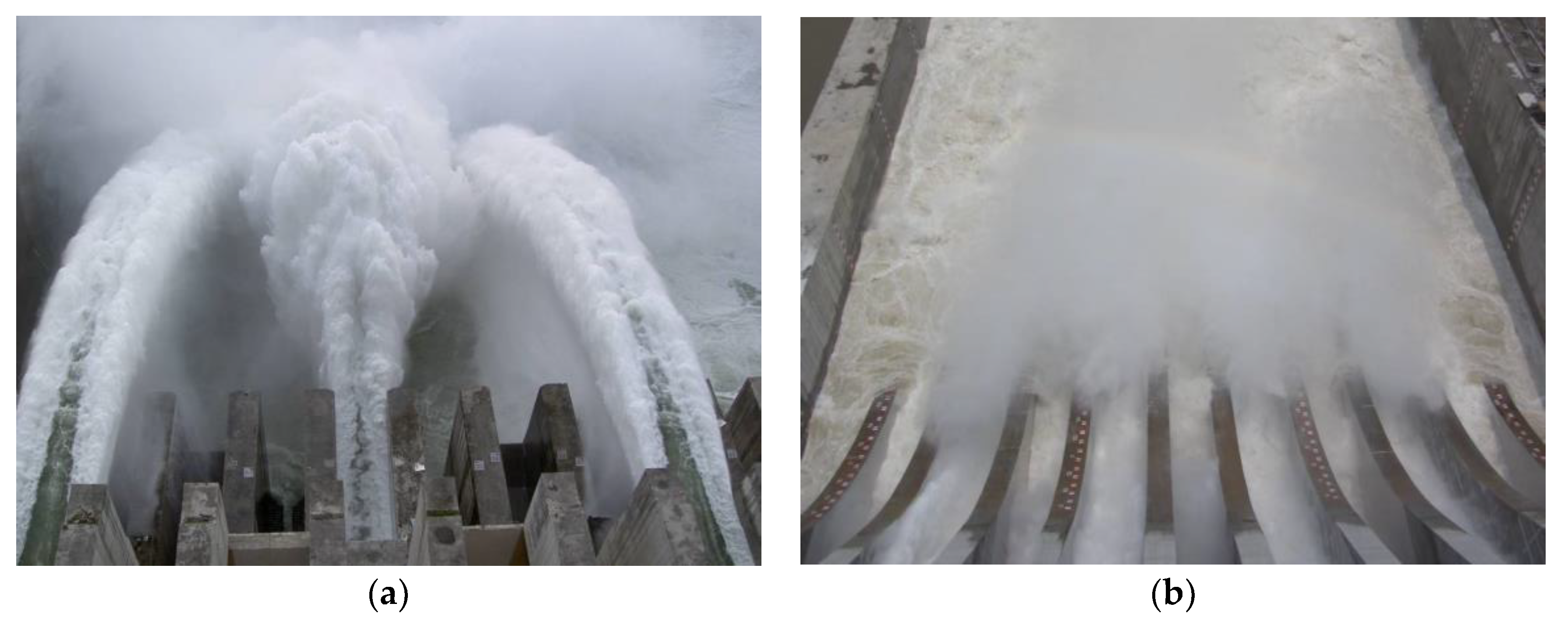
Cavitation erosion caused by high velocity flows is a common phenomenon in spillways or chutes with high-head dams. A commonly adopted counter-measure to reduce or prevent cavitation damage is aeration [1,2,3,4,5,6]. Three-dimensional aerators are used to enhance air entertainment into water and to prevent cavitation erosion on spillways. Full interfacial aeration is commonly observed at the free surface of the upper, lower and side nappe along the free jet (Figure 1). The effect of air entrainment is based on the jet disintegration process due to turbulence and secondary interactions with the surrounding atmosphere.
Air entrainment at the interfacial area is a fundamental parameter in numerical models for simulating two-phase flows. Likewise, it is also an essential consideration when designing optimum aerators. During the last few decades, numerous studies have been conducted to investigate the air concentration and free-surface aeration on an aerator. A series of experiments were conducted to study the free-surface aeration and diffusion characteristics of the bottom aeration devices [7,8,9,10,11]. Results indicate that the quantities and geometric scales of air bubbles are important parameters in characterizing the air concentration in the interfacial area. Chanson [12] described the flow structure of the developing aerated region in a flat chute and found that the maximum mean air content in different cross-sections was 12%. Toombes [13] showed that the maximum bubble count rates typically correspond to air concentration between 40% and 60%. The distribution of velocity indices at the different nappes, which stays at the downstream of an expanding chute aerator, were found to be different [14] and a solution was also found to improve both the bottom and lateral cavities’ length [15]. The longitudinal position of the upper trajectory apex was found to be further downstream than that of the lower trajectory apex [16]. Kramer and Hager [17] found that both the entrainment rate and dimensionless bubble count rate increased with jet length. The mean air concentration is affected by aerators, but the air concentration at the bottom is limited [18]. Furthermore, Toombes and Chanson [19] studied flows past a backward-facing step, where the void fraction distribution, bubble count rate, local air distribution and water chord size were indicated. The results showed that the relationship between bubble count rate and void fraction can be defined by a quasi-parabolic function, while probability density functions of local chord size exhibited a quasi-log-normal shape. Some researchers [20,21,22,23,24] also established analytical equations to predict the air concentration distributions at the aerators’ downstream. Numerical models such as the lattice Boltzmann method were found to successfully simulate two-phase flows and free-surface flows [25,26,27]. These models may be used to complement physical models and experimental measurements after careful validation and verification of model parameters such as the void fraction distribution, velocity, and air-bubble chord sizes. Chanson [28] reviewed the recent progress in turbulent free-surface flows and the mechanics of aerated flows and highlighted that physical modelling tests are efficient methods to validate phenomenological, theoretical and numerical models.
Although numerous studies regarding air–water flows have been conducted over the years, only a few researchers, however, have systematically investigated the air bubble count rate and bubble size of high velocity air–water flows downstream of the pressure outlet joined by a three-dimensional aerator (sudden vertical drop and lateral enlargement) in the tunnel. There is also a lack of knowledge regarding the influence of the bubble count rate and bubble size on the air concentration in two-phase flows, which is necessary for improving turbulence models. Thus, further insight is needed regarding the details of air entrainment in high-speed flows and the related core area features. In this study, a series of experimental investigations were systematically conducted to further the knowledge of air water flows among the upper, lower and side nappes downstream of a three-dimensional aerator (Figure 2). The experimental data and equations obtained from this study provide novel information and a quantitative description of the aeration flow structure at the high-speed interfacial area.
2. Experimental Setup
Experiments were performed at the State Key Laboratory of Hydraulic and Mountain River Engineering, Sichuan University, China. The experimental setup (Figure 3) includes an upstream reservoir, a pressure section, a sudden vertical drop and lateral enlargement aerator, a free flow section, a tail-water section, and an underground reservoir. Water is discharged (can be up to 0.5 m3/s) by a continuous and stable water supply system (2.5 m wide, 3.5 m long, and 6.3 m high). The components of the pressure inlet were assembled with a smooth steel plate. The pressure section is a rectangular pipe (0.25 m wide, 0.15 high and 2.0 m long) with a variable inclination angle varied with the downstream chute. The sudden fall-expansion aerator (height h × width b) was installed at the end of the pressure section. The free-flow section was fabricated from polymethyl methacrylate (PMMA) with a roughness height of 0.008 mm. The upper, lower, and side nappes were exposed to atmospheric pressure. The constant water levels corresponding to a particular head were maintained in the upstream reservoir.
Experiments were carried out for mean velocities (V0) of 6 m/s, 7 m/s, 8 m/s, and 9 m/s; chute slopes of 0%, 10%, and 25%; and aerator sizes (h, b) of 0.025m, 0.045m, and 0.065 m. The test cases are summarized in Table 1 (0.9 < qw < 1.35, 0.89 < Re < 1.34). It should be noted that some combinations (series 7–10, and 13 in Table 1) pertain to cases involving three-dimensional (vertical drop and lateral enlargement) aerators. The other cases involve only either vertical drop aerators or lateral enlargement aerators. Upstream flows were supercritical (4.95 < Fr < 7.42) for all of the investigated flow conditions. Downstream of the aerator, a free jet, with the use of a ventilated air cavity below and/or beside it, was formed.
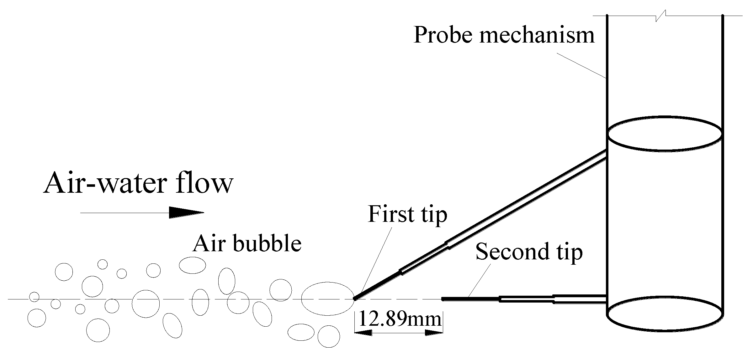
The air concentration, bubble count rate, and chord length were recorded using a CQY—Z8a measurement instrument [14,29,30] with a double-tip conductivity probe (Figure 4). Different voltage indices between air and water were measured by the platinum tip. The probe consisted of two identical tips, including an external stainless steel electrode with 0.7-mm-diameter and an internal concentric platinum electrode with 0.1-mm-diameter. The tips are aligned in the flow direction and the distance between the two tips is 12.89 mm. Both tips were connected to an electronics device with a response time less than 10 μs. The vertical translation of the probe was dominated by a fixed device with an accuracy of 1 mm. The probe measurements were taken at regular intervals of 5 mm along the vertical direction from the chute bottom to the free surface (or side nappe surface) and 100 mm along the flow direction. At each location, signals were recorded at a scan rate (f) of 100 kHz per channel for a scan period () of 10 s. The scan period was based on the findings of Toombes [13] which indicated that a scanning period of 10 s was long enough to provide a reasonable representation of the flow characteristics while maintaining realistic time and data storage constraints.
Figure 4 presents a typical aeration structure detected by a probe at a fixed location along the aeration flow. Assuming each segment is either air or water, the air concentration can be presented as the probability of any discrete element being air. The air concentration is computed as the encountering air’s probability at the leading tip of the probe.
The number of data (N) can be obtained by multiplying the frequency (f) of the measurement instrument with the sampling time T, i.e., . Those data were classified according to two categories, air and water signals. The air concentration () was computed as the encountering air’s probability at the leading tip of the probe, which can be expressed as [26]
where Ri represents the ratio of bubbles measured all throughout the whole measurement time. When the probe tip is completely immersed in air bubbles Ri = 1, otherwise Ri = 0.
The length of bubble chord is defined as the straight distance between the two intersections of the interface [12]. Note that an air bubble is defined as a volume of air (i.e., air entity), which can be detected by the leading tip of the probe between two continuous air–water interface events. The bubble chord length is calculated by
where is the number of detected bubbles recorded; and is the bubble velocity equal to the local mean aeration velocity (i.e., no slip between the air and water phases).
3. Results
The air bubble frequency and chord length are two important parameters used to characterize the air concentration of aerated flows. We first describe air bubble frequency among the upper, lower and side air–water mixed layers in the experimental flows with various conditions. In this section, the relationships between air concentration with air bubble frequency, and with the relative location at which the maximum air bubble frequency are also discussed. Next, we identify the effects of initial flow velocity on air bubble chord length. In addition, the relationships between the air concentration and air bubble chord length, and between air bubble count rate and air bubble size are also evaluated.
3.1. Air Bubble Frequency
The air bubble frequency characterizes the flow fragmentation, which is proportional to the specific area of the interface between two phases. The air bubble frequency, or air bubble count rate, is a function of bubbles’ shape and size, surface tension, and shear forces of the fluid. Predicting how air concentration affects the bubble frequency is a complex problem [19]. A simplified analogy would be to consider on aeration flows past a fixed probe, as a series of discrete one-dimensional air and water elements (Figure 4). Here, the air bubble frequency (Fa) is defined as the number of air-structures (Na) per unit time () detected by the leading tip of the probe sensor (i.e., Fa = Na/t).
Typical air bubble frequency distributions at each cross-section along the upper, lower, and side nappes are presented in Figure 5. The air bubble frequency distributions exhibit unitary self-similarity along the thickness of the mixed layer and the horizontal distance. The trend of the cross-sectional distribution tends to initially increase and then decrease from the aeration interface to the inside of the water following a Gaussian distribution that is defined by the following functions:
where, is the dimensionless air bubble frequency and is the maximum bubble frequency in the cross-section; The characteristic value of μ0 reflects the depth corresponding to the air bubble frequency; σ0 represents the degree of deviation between the relative depth and its mean value.
For all experimental results, the air bubble frequency distributions correspond well with the data reported by Toombes and Chanson [19], as illustrated in Figure 5. Figure 6 presents a plot of experimental data, , with calculated non-dimensional air bubble frequency using Equation (3). The calculated results at upper, lower, and lateral nappes were in qualitative agreement with experimental data, although there was some scatter. It is noted that the characteristic values of and differed among the upper, lower, and side nappes (Table 2). For the upper nappe, the air bubbles do not easily diffuse and instead transport to the inside of the water due to the buoyancy. This result in the air bubbles being drawn closer to the free surface (). For the side nappe, the air bubbles can easily diffuse and transport to the interior of the water () because of the effect of large transverse turbulent diffusion [15]. For the lower nappe, the air bubbles are dragged by the buoyant force to the interior of the water ().
Air concentration distribution is just the external manifestation of air–water flows, whereas the internal factors include the count rate and size of the air bubbles. So, it is crucial to understand the features of the air bubble frequency and the air bubble chord length.
The air bubble frequency distributions at various positions along the jet obtained in this study and those reported by Chanson [12] and Toombes and Chanson [19] are shown in Figure 7. It is evident that the air bubble frequency initially increases and then decreases with the increase of air concentrations in the upper, lower, and side nappes. At each cross-section, the air bubble frequency profiles reach to an apex which corresponds to air concentrations of approximately 50%. The profiles tend to zero at extremely low and extremely high air concentrations. Overall, the distributions of the dimensionless air bubble frequency can be well fitted by the parabolic function:
Qualitatively, the calculated results of Equation (4) correspond with the results of Chanson [12] and Toombes and Chanson [19] (Figure 7). It is worth noting that the data [12] slightly deviate from the fully developed supercritical flows, suggesting that Equation (4) has broad applicability.
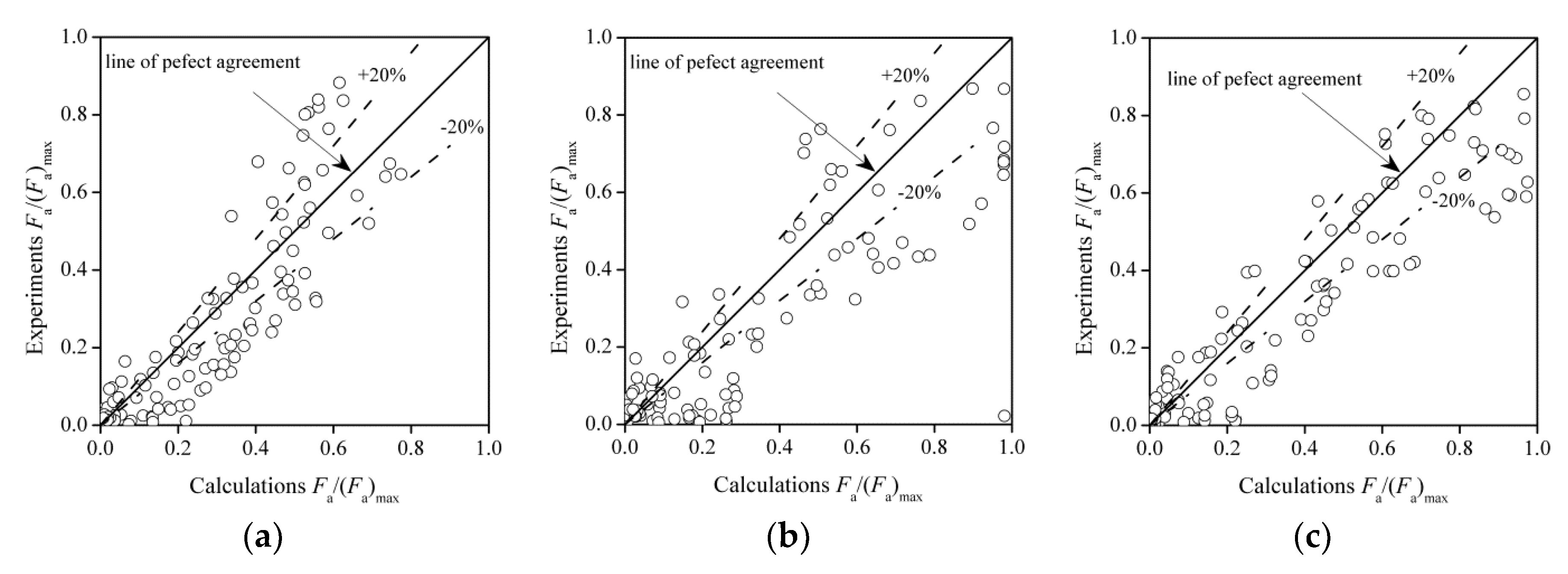
The majority of the data fall within the ±20% error lines as shown in Figure 8. The calculated non-dimensional air bubble frequency using Equation (4) are in reasonably good agreement with the experimental data at upper, lower, and lateral nappes.
The relationships between air concentration and the relative distance, which corresponds to the maximum air bubble frequency are presented in Figure 9 where a large fluctuation of air concentration () in the initial regime of aeration can be observed. The fluctuation may be due to the aeration layer located close to the pressure outlet, which may be thin and unstable. The air–water layer becomes stable with the development of the aeration further downstream. The air concentration corresponding to the maximum air bubble frequency gradually moves toward to 50% line. The result is consistent with the findings of Figure 7. Actually, the maximum air bubble frequency does not always coincide with accurately. Factors such as the average size and length scales of discrete air and water elements may affect the local air concentration and flow conditions in air–water flows [13,31].
The relative location corresponding to the maximum air bubble frequency is shown in Figure 10. It can be seen that the relative location of the maximum air bubble frequency is 0.210, 0.326 and 0.283 times the thicknesses of the air–water layers in the upper, lower and side nappes, respectively. The results are consistent with the results of Figure 5. For the upper nappe, the air can easily be drawn into the water because the air–water external interface directly interacts with the atmosphere. However, the air bubbles cannot easily diffuse and transport to the inside of the jet because of the effect of buoyancy. For the lower nappe, the air bubbles can easily diffuse and move into the interior of the jet due to the local air rotation and eddy currents, which are driven by the air–water interfacial turbulence coupled with the positive effect of buoyancy.
3.2. Air Bubble Chord Length Distributions
Air bubble size is another parameter reflecting the characteristics of air–water flows. It is difficult to measure the size of air bubbles since their shapes vary greatly, are complex and highly changeable. This value can only be indirectly determined from the bubble chord length which is obtained using the double-tip conductivity probe. Here, the chord length (chab)mean is adopted to assess the size of the air bubbles, which is defined as follows:
where nj is the count of air bubbles in the bubble chord length interval Δ(chab)j (Δ(chab)j =0.1mm in the experiments); and (chab)j is the average value of the chord length interval (e.g., the probability of chord length from 1.0 to 1.1 mm is represented by the label 1.05 mm).
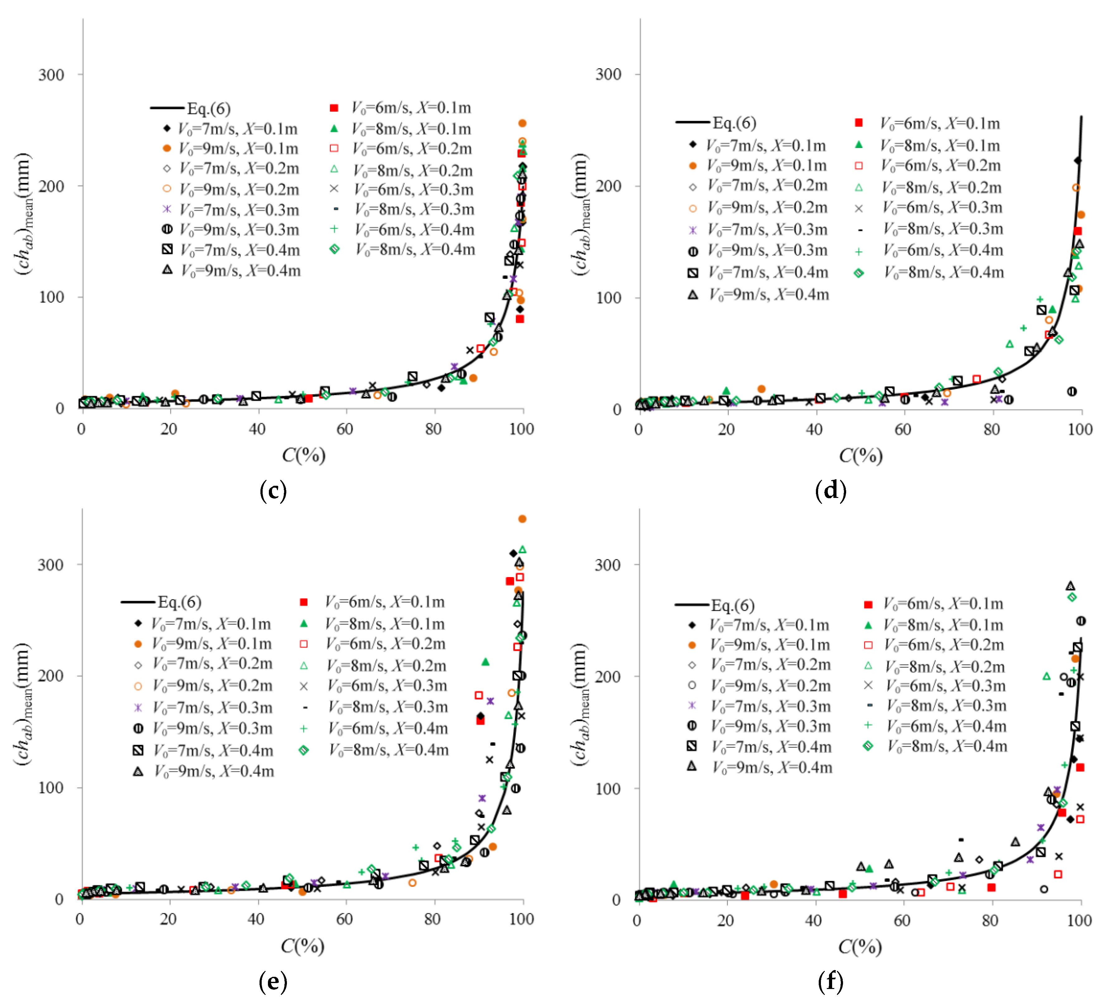
The air bubble chord lengths (chab)mean are presented in Figure 11 at various positions in the upper, lower and side nappes. It is note that the air bubble chord length distributions obtained at the upper, lower, and side nappes have similar shapes. The air bubble chord length in the vicinity of the air–water interface is largest and then gradually decreases toward the inside of the water. A broad spectrum of air bubble chord lengths, i.e., from less than 0.1 mm to greater than 100 mm, is observed at each location and cross-section. At high air concentration (i.e., ), chord length of many air bubbles can reach up to 100 mm or even more. These large values may be large air packets and air volumes surrounding the water structure (e.g., droplets). The reason is that the regime with high air concentration is always close to the air–water interfaces, which become uneven under the influence of turbulent forces. Air in the vicinity of the free surface that are trapped by the generated waves were treated as air bubbles by the conductivity probe. In addition, the shape of the air bubble is not completely spherical, in most cases, it is oval or banding, causing it to be measured to be much larger than it actually is. Indeed, it is nearly impossible to distinguish between air-bubbles and an un-enclosed bubble structure. The results indicate that the large air bubbles are constantly sheared and tore as they move towards the interior of the water. This results in air bubbles located deeper inside the body of water to be much smaller in size. Figure 9 also suggests that for C < 90%, bubble chord lengths will most likely be no more than 20 mm and that bubbles close to the pressure outlet will have small sizes.
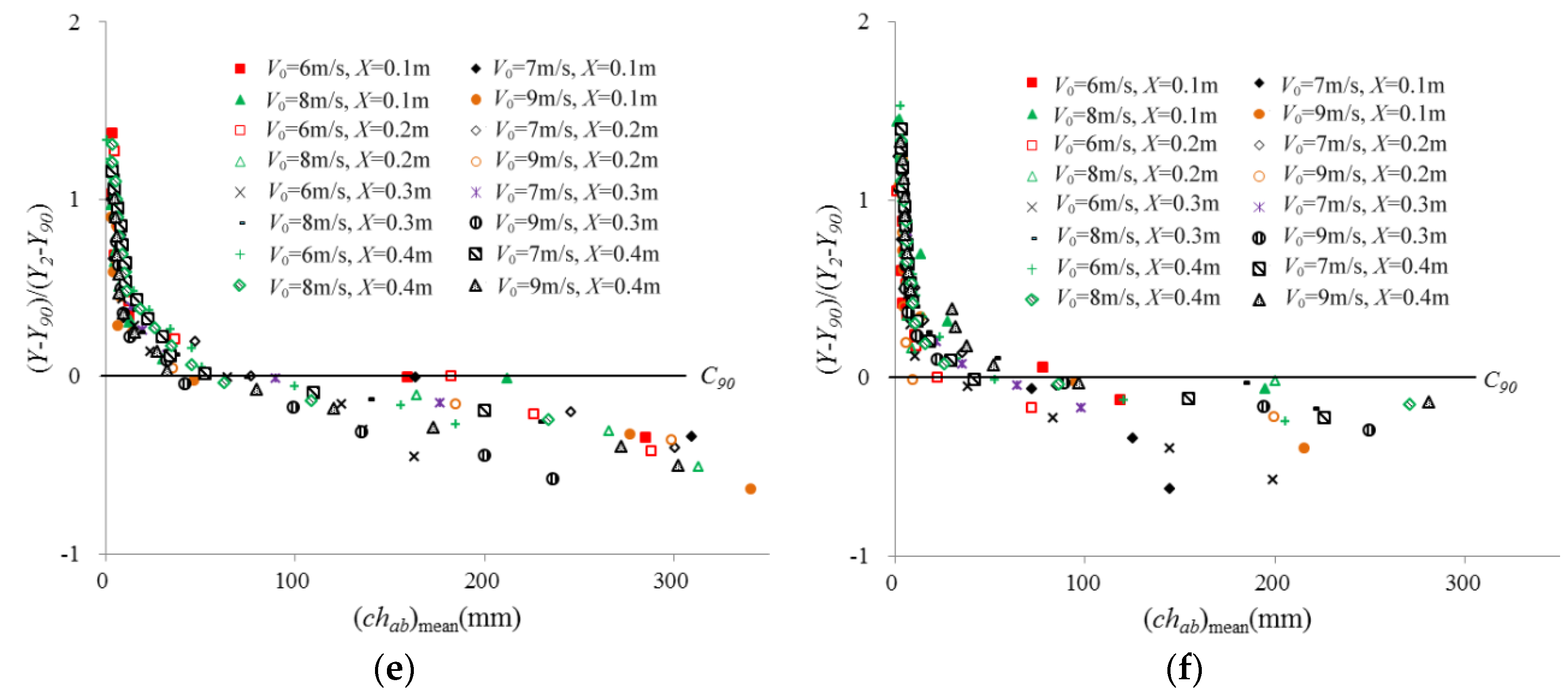
A positive correlation is observed between the air concentration and air bubble chord length among the upper, lower and side nappes (Figure 12). The distribution can be defined according to the function:
where , and are empirical coefficients that may be related to the interaction. For the present experimental data, , and were used. The coefficients of determination were set to be 0.85. 0.93 and 0.91 for the upper, lower and side nappes respectively.
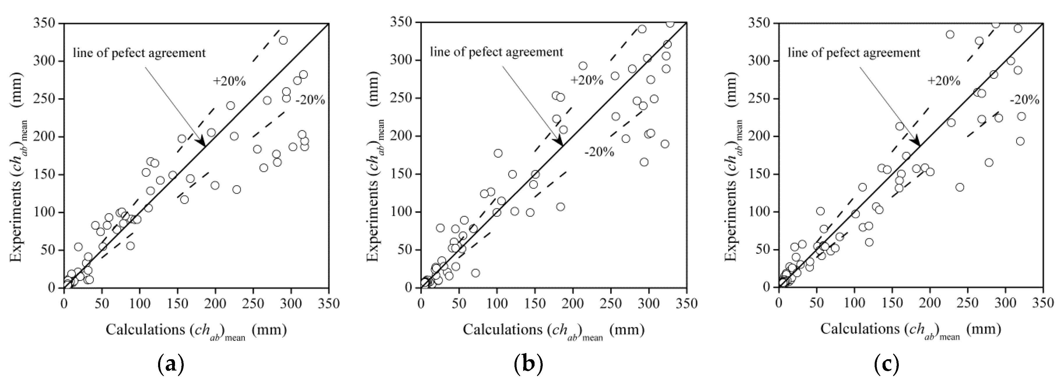
Figure 13 presents a plot of experimental data, (chab)mean, with calculated results using Equation (6). Since most of the values of (chab)mean calculated from Equation (6) fall around the line of perfect agreement in an area within ±20% error lines, although some discrepancy exists. The results exhibit agreement with the theoretical distribution curve of Equation (6) for all flow conditions at various positions.
As the relationships between the air concentration and air bubble frequency, as well as the air bubble chord length have been discussed above, the relationship between the air bubble count rate and bubble size is also considered (Figure 14). It is evident that the correlations are clearly non-symmetric, unimodal and positively skewed and may therefore be represented by a probability density function defined by the Gamma distribution. According to mathematical statistics, the gamma distribution is a continuous probability function that can be written as follows:
where is the shape parameter, is the scale parameter, and is the gamma Function, and .
Equation (7) is a classic two-parameter gamma distribution. Considering the complexity of the air bubble frequency and chord length in aeration flows, the five-parameters form of the generalized gamma distribution (also known as the generalized gamma function with four parameters after translation) is used in this study. The probability density function is written as follows:
where and are the coefficients; , , , , and are the five parameters, of which and denote the shape parameters, and denote the scale parameters, and is the threshold parameter; and is the gamma function.
Based on the experimental data and the theoretical distribution curve of Equation (8), the relationship between the air bubble frequency and air bubble chord length can be fitted as follows:
Examples of a “modified” five-parameters gamma distribution that were used to fit the air bubble chord length distributions (Figure 14). The data is reasonably well represented by a “modified” gamma function distribution, although there is significant scatter.
Additionally, Figure 15 presents a plot of experimental data, , with calculated non-dimensional air bubble frequency using Equation (9). Since most of the values of calculated from Equation (9) fall around the line of perfect agreement in an area within ±20% error lines, suggesting that Equation (9) can be considered adequate in calculating the air bubbles chord length distribution. The “modified” gamma function is skewed to the left with a peak that lies in the small chord size values. The mode was found to be between 0.5 and 30 mm.
4. Discussion
Air concentration is a macro parameter that is used to describe air–water flows. However, it is still insufficient in providing insight that would lead to a deeper understanding of the said phenomena. The process of aeration defines the general developing process of air moving into a body of water, i.e., the air bubbles. As such, the micro characteristics of air bubbles such as its count rate and size are crucial parameters in the study of aeration flows.
A double-tip conductivity probe used in present study to detect the air–water interfaces at different fixed points downstream of a three-dimensional (vertical drop and lateral enlargement) aerator. Some simple expressions were developed to simulate the distributions of air bubble frequency and bubble chord sizes. The relationships between the air concentration, the air bubble frequency and the air bubble chord length were also established. The obtained air concentration distributions satisfy the analytical model of Chanson [12], Equation (4) for air bubble frequency distributions as observed in supercritical open channel flows and backward-facing step flows (Toombes and Chanson [19]). A “modified” gamma probability density function was found to provide a good fit to the air bubble chord length distributions measured from three-dimensional aerator flows. This is different from the log-normal probability density functions that Chanson (1997) used for supercritical open channel flows. The distributions of the air bubble chord length showed a positive correlation with the void fraction.
Physical modelling may provide some information on the flow motion if a suitable dynamic similarity is selected. Air–water flows depend on Froude, Reynolds, and Weber numbers. Strictly speaking, dynamic similarity of air concentration and air bubble dissipation for free-surface aeration on aerator flows on a reduced-scale model is not possible (Chanson [32]) because it is impossible to satisfy simultaneously Froude and Reynolds similarities. Hence, the experimental results cannot be directly extrapolated to prototypes unless working at full scale. Nevertheless, with the assumption of Froude similarity, the Reynolds number (Re) should be larger than 1 × 10⁵ to minimize the scale effects (Chanson [32]; Heller [33]). This limit is considered in the present study (Re ~ 0.89–1.34 × 10⁶). Actually, results from scale experiments using Froude similarity are on the safe side for engineers with respect to air concentrations due to aeration tends to be underestimated in the smaller experiments.
Due to the complexity of bubble distribution in the air–water interfaces, the present results only serve as a preliminary investigation of the air bubble properties in the air–water mixtures downstream of a three-dimensional aerator. Hence, more detailed research is needed to study the air bubbles in aeration flows.
5. Conclusions
A number of experiments were performed under various configurations and approach flow velocities for a 3D aerator. The air concentration, air bubble frequency and bubble chord length were recorded in the developing shear layer of the upper, lower and side nappes downstream. The results are summarized as follows:
- (1)
- The air bubble frequency distributions (yielding to the Gauss function) exhibit a unitary self-similarity along the air–water layer, presenting a trend which initially increases and then decreases from the air–water interface to the inside of the water. A quasi-parabolic relationship between the air bubble frequency and the air concentration is obtained for the upper, lower and side nappes.
- (2)
- The air bubble frequency reaches to apex at approximately C = 50%, and then decreases to zero as C = 0% and C = 100%. The relative location at which the maximum air bubble frequency is observed is at 0.21, 0.326 and 0.283 times of the thickness of the air–water layers for the upper, lower and side nappes, respectively.
- (3)
- The air bubble chord length decreases gradually from the free interface to the interior of the water. When the air bubble chord size is plotted against the air concentration, the resulting distribution follows a power-law function. The relationship between the air bubble frequency and bubble chord size exhibits a “modified” gamma function for the upper, lower and side nappes.
Author Contributions
S.L. and J.Z. proposed the research ideas and methods of the manuscript and writing, X.C. put forward the revise suggestion to the paper. J.C. is responsible for data collection and creating the figures.
Funding
This research was funded by the Chinese Scholarship Council (CSC), grant number 201804910306; the CAS “Light of West China” Program, grant number Y6R2220220; the National Science Fund for Distinguished Young Scholars, grant number 51625901; and the Natural Science Foundation of China, grant number 51579165.
Conflicts of Interest
The authors declare no conflicts of interest.
Notations
The following symbols are used in this paper:
| empirical coefficients | |
| b | the width of sudden fall-expansion aerator |
| B | width of the pressure outlet |
| air concentration | |
| the air bubble chord length size | |
| the average value of air bubble chord length | |
| air bubble chord length | |
| i | air bubble number |
| air bubble frequency | |
| the maximum bubble frequency | |
| Fr | Froude Number |
| g | gravitational acceleration |
| h | the height of sudden fall-expansion aerator |
| H | height of the pressure outlet |
| the unit-width discharge | |
| Reynolds number | |
| the number of detected bubbles | |
| the count of air bubbles | |
| the number of air-structures | |
| Ri | a ratio of the bubble measured in the whole measurement time |
| t | time |
| the cross-sectional mean velocity at the pressure outlet | |
| X, Y, Z | the horizontal, transverse and vertical coordinates of the lower nappe profile |
| the slope with respect to the horizontal downstream bottom plane | |
| Y2, Z2 | characteristic air–water flow heights where the air concentration C = 2%; |
| Y90, Z90 | characteristic air–water flow heights where the air concentration C = 90% |
| characteristic depth corresponding to the air bubble frequency | |
| degree of deviation between the relative depth and its mean value | |
| the probability density function of the gamma function | |
| the shape parameter | |
| the scale parameter | |
| the gamma function |
References
- Cassidy, J.; Elder, R. Spillways of High Dams, Developments in Hydraulic Engineering—2; Elsevier: New York, NY, USA, 1984. [Google Scholar]
- Kells, J.A.; Smith, C.D. Reduction of cavitation on spillways by induced air entrainment. Can. J. Civ. Eng. 1991, 18, 358–377. [Google Scholar] [CrossRef]
- Hager, W.H.; Pfister, M. Historical advance of chute aerators. In Proceedings of the 33rd IAHR Congress, Vancouver, BC, Canada, 9–14 August 2009; pp. 5827–5834. [Google Scholar]
- Pfister, M.; Lucas, J.; Hager, W.H. Chute aerators: Pre aerated approach flow. J. Hydraul. Eng. 2011, 137, 1452–1461. [Google Scholar] [CrossRef]
- Hager, W.H.; Boes, R.M. Hydraulic structures: A positive outlook into the future. J. Hydraul. Res. 2014, 52, 299–310. [Google Scholar] [CrossRef]
- Low, H.S. Model Studies of Clyde Dam Spillway Aerators; Research Report, No. 86-6; Department of Civil Engineering, University of Canterbury: Christchurch, New Zealand, 1986. [Google Scholar]
- Zhang, J.M.; Wang, Y.R.; Yang, Q.; Xu, W.L. Scale effects of incipient cavitation for high-speed flows. Proc. Inst. Civ. Eng. Water Manag. 2013, 166, 141–145. [Google Scholar] [CrossRef]
- Chanson, H. A study of Air Entrainment and Aeration Devices on a Spillway Model. Ph.D. Thesis, Department of Civil Engineering, University of Canterbury, Christchurch, New Zealand, 1988. [Google Scholar]
- Chanson, H. Air Bubble Entrainment in Free-Surface Turbulent Flows: Experimental Investigations; Research Report No. CH46/95; Department of Civil Engineering, University of Queensland: Brisbane, Australia, 1995. [Google Scholar]
- Chanson, H.; Brattberg, T. Experimental Investigations of Air Bubble Entrainment in Developing Shear Layer; Research Report, No. CH48/97; Department of Civil Engineering, The University of Queensland: Brisbane, Australia, 1997. [Google Scholar]
- Brattberg, T.; Chanson, H.; Toombes, L. Experimental investigations of free-surface aeration in the developing flow of two-dimensional water jets. J. Fluids Eng. 1998, 120, 738–744. [Google Scholar] [CrossRef]
- Chanson, H. Air bubble entrainment in open channels: Flow structure and bubble size distributions. Int. J. Multiphase Flow 1997, 23, 193–203. [Google Scholar] [CrossRef] [Green Version]
- Toombes, L. Experimental Study of Air-Water Flow Properties on Low-Gradient Stepped Cascades. Ph.D. Thesis, Department of Civil Engineering, University of Queensland, Brisbane, Australia, 2002. [Google Scholar]
- Li, S.; Zhang, J.M.; Chen, X.Q.; Zhou Gordon, G.D. Air concentration and velocity downstream of an expanding chute aerator. J. Hydraul. Res. 2018, 56, 412–423. [Google Scholar] [CrossRef]
- Li, S.; Zhang, J.M.; Chen, X.Q.; Chen, J.G.; Zhou Gordon, G.D. Cavity length downstream of a sudden fall-expansion aerator in chute. Water Sci. Technol. Water Supply 2018, 18, 2053–2062. [Google Scholar] [CrossRef]
- Pfister, M.; Hager, W.H. Deflector-generated jets. J. Hydraul. Res. 2009, 47, 466–475. [Google Scholar] [CrossRef]
- Kramer, K.; Hager, W.H. Air transport in chute flows. Int. J. Multiphase Flow 2005, 31, 1181–1197. [Google Scholar] [CrossRef]
- Pfister, M.; Hager, W.H. Chute aerators. I: Air transport characteristics. J. Hydraul. Eng. 2010, 136, 352–359. [Google Scholar] [CrossRef]
- Toombes, L.; Chanson, H. Interfacial aeration and bubble count rate distributions in a supercritical flow past a backward-facing step. Int. J. Multiphase Flow 2008, 34, 427–436. [Google Scholar] [CrossRef] [Green Version]
- Zhang, J.M.; Chen, J.G.; Xu, W.L.; Wang, Y.R.; Li, G.J. Three-dimensional numerical simulation of aerated flows downstream sudden fall aerator expansion-in a tunnel. J. Hydrodyn. Ser. B 2011, 23, 71–80. [Google Scholar] [CrossRef]
- Toombes, L.; Chanson, H. Free-surface aeration and momentum exchange at a bottom outlet. J. Hydraul. Res. 2007, 45, 100–110. [Google Scholar] [CrossRef] [Green Version]
- Fuhrhop, H.; Schulz, H.E.; Wittenberg, H. Solution for spillway chute aeration through bottom aerators. Int. J. CMEM 2014, 2, 298–312. [Google Scholar] [CrossRef] [Green Version]
- Bai, Z.L.; Peng, Y.; Zhang, J.M. Three-Dimensional Turbulence Simulation of Flow in a V-Shaped Stepped Spillway. J. Hydraul. Eng. 2017, 143, 06017011. [Google Scholar] [CrossRef]
- Duarte, R. Influence of Air Entrainment on Rock Scour Development and Block Stability in Plunge Pools. Ph.D. Thesis, EPFL-LCH, Lausanne, Switzerland, 2014. [Google Scholar]
- Peng, Y.; Mao, Y.F.; Wang, B.; Xie, B. Study on C-S and P-R EOS in pseudo-potential lattice Boltzmann model for two-phase flows. Int. J. Mod. Phys. C 2017, 28. [Google Scholar] [CrossRef]
- Peng, Y.; Wang, B.; Mao, Y.F. Study on force schemes in pseudopotential lattice Boltzmann model for two-phase flows. Math. Probl. Eng. 2018, 2018, 6496379. [Google Scholar] [CrossRef]
- Peng, Y.; Zhang, J.M.; Meng, J.P. Second order force scheme for lattice Boltzmann model of shallow water flows. J. Hydraul. Res. 2017, 55, 592–597. [Google Scholar] [CrossRef]
- Chanson, H. Hydraulics of aerated flows: Qui pro quo? J. Hydraul. Res. 2013, 51, 223–243. [Google Scholar] [CrossRef]
- Chen, X.P.; Shao, D.C. Measuring bubbles sizes in self-aerated flow. Water Res. Hydropower Eng. 2006, 37, 33–36. [Google Scholar]
- Bai, R.; Liu, S.; Tian, Z.; Wang, W.; Zhang, F. Experimental Investigation of Air–Water Flow Properties of Offset Aerators. J. Hydraul. Eng. 2017, 144, 04017059. [Google Scholar] [CrossRef]
- Gonzalez, C.A. An Experimental Study of Free-Surface Aeration on Embankment Stepped Chutes. Ph.D. Thesis, Department of Civil Engineering, The University of Queensland, Brisbane, Australia, 2005. [Google Scholar]
- Chanson, H. Turbulent air-water flows in hydraulic structures: Dynamic similarity and scale effects. Environ. Fluid Mech. 2009, 9, 125–142. [Google Scholar] [CrossRef] [Green Version]
- Heller, V. Scale effects in physical hydraulic engineering models. J. Hydraul. Res. 2011, 49, 293–306. [Google Scholar] [CrossRef]
Figure 1.
Air water flow in three-dimensional aerators: (a) Three Gorges Project; (b) Xiang Jia-Ba Project.
Figure 1.
Air water flow in three-dimensional aerators: (a) Three Gorges Project; (b) Xiang Jia-Ba Project.

Figure 2.
Schematic with the relevant parameters: (a) side view and (b) plan view.

Figure 3.
Sketch of the experimental model and test equipment.
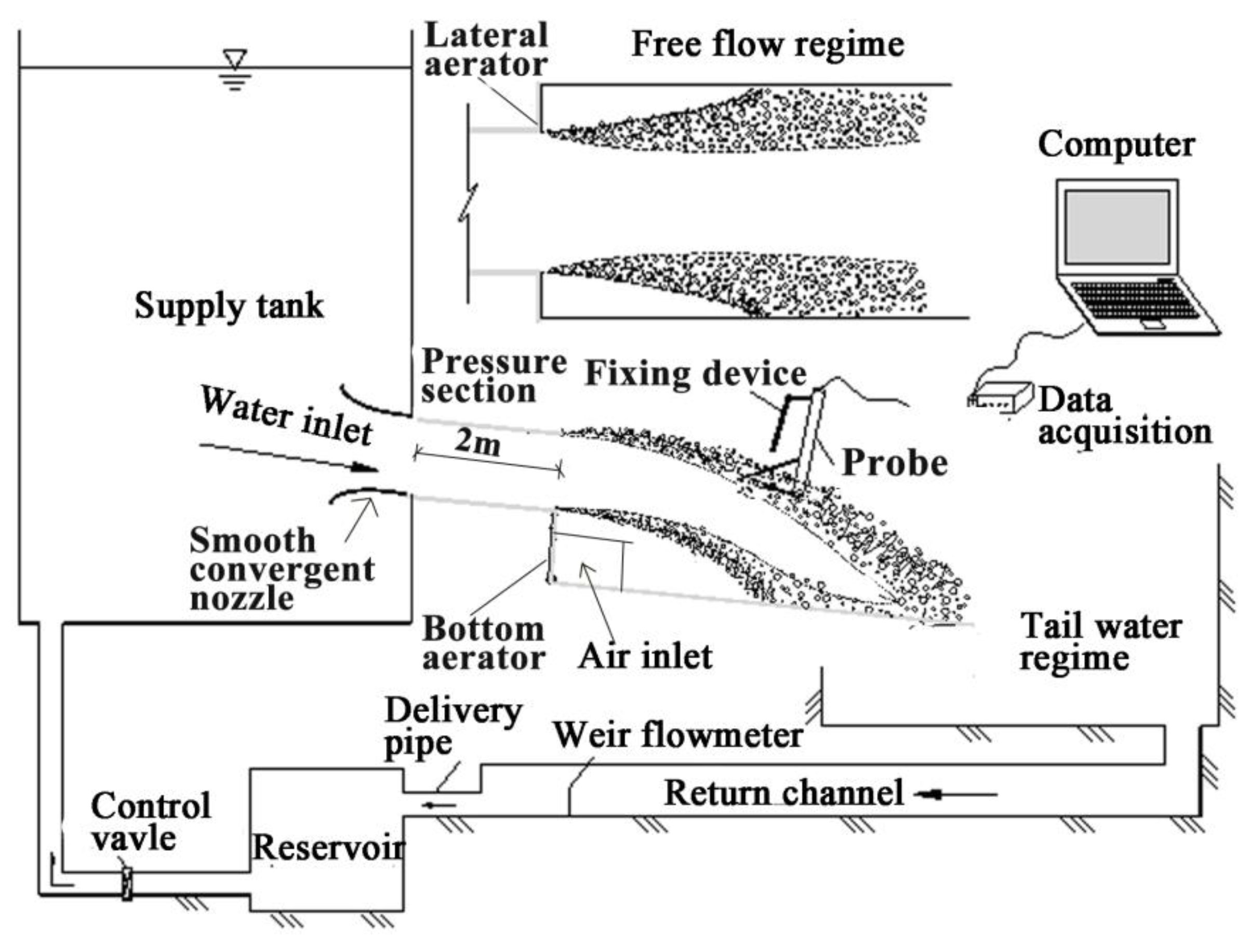
Figure 4.
Sketch of the double-tip conductive probe.

Figure 5.
Air bubble frequency distributions compared with the theoretical distribution obtained from Equation (3). Upper nappe (a) (h, b) = (4.5 cm, 4.5 cm), θ = 25%. (b) (h, b) = (6.5 cm, 6.5 cm), θ = 10%; lower nappe (c) (h, b) = (4.5 cm, 4.5 cm), θ = 25%. (d) (h, b) = (6.5 cm, 6.5 cm), θ = 10%; side nappe (e) (h, b) = (4.5 cm, 4.5 cm), θ = 25%. (f) (h, b) = (6.5 cm, 6.5 cm), θ = 10%.


Figure 6.
Comparison of Equation (3) with the experimental data. (a) upper nappe; (b) lower nappe; (c) side nappe.
Figure 6.
Comparison of Equation (3) with the experimental data. (a) upper nappe; (b) lower nappe; (c) side nappe.

Figure 7.
Dimensionless air bubble frequency as a function of the air concentration fitted with Equation (4). Upper nappe (a) (h, b) = (4.5 cm, 4.5 cm), θ = 25%. (b) (h, b) = (6.5 cm, 6.5 cm), θ = 10%; lower nappe (c) (h, b) = (4.5 cm, 4.5 cm), θ = 25%. (d) (h, b) = (6.5 cm, 6.5 cm), θ = 10%; side nappe (e) (h, b) = (4.5 cm, 4.5 cm), θ = 25%. (f) (h, b) = (6.5 cm, 6.5 cm), θ = 10%.

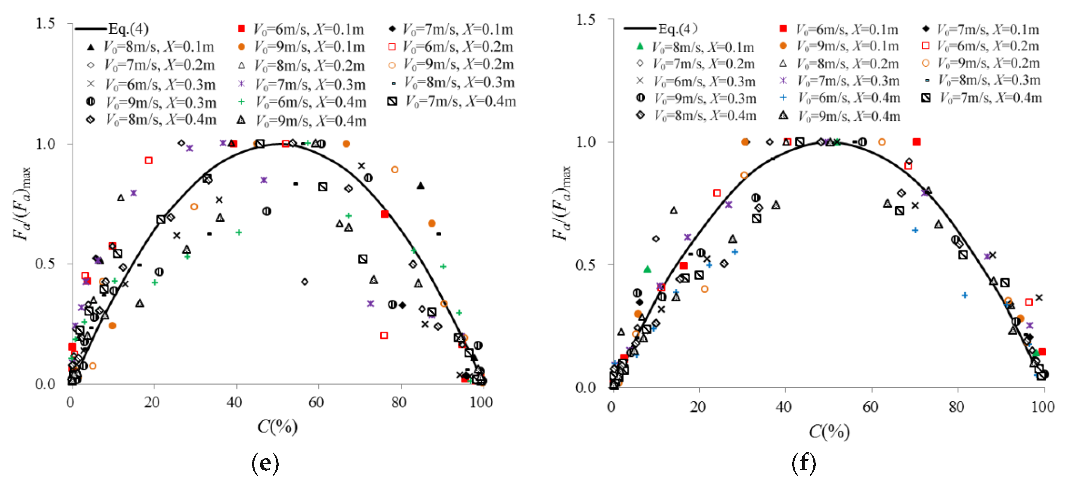
Figure 8.
Comparison of experimental data with calculated values of dimensionless air bubble frequency. (a) upper nappe; (b) lower nappe; (c) side nappe.
Figure 8.
Comparison of experimental data with calculated values of dimensionless air bubble frequency. (a) upper nappe; (b) lower nappe; (c) side nappe.

Figure 9.
Air concentration corresponding to the maximum air bubble frequency. Upper nappe (a) (h, b) = (4.5 cm, 4.5 cm). (b) θ = 10%; lower nappe (c) (h, b) = (4.5 cm, 4.5 cm). (d) θ = 10%; side nappe (e) (h, b) = (4.5 cm, 4.5 cm). (f) θ = 10%.
Figure 9.
Air concentration corresponding to the maximum air bubble frequency. Upper nappe (a) (h, b) = (4.5 cm, 4.5 cm). (b) θ = 10%; lower nappe (c) (h, b) = (4.5 cm, 4.5 cm). (d) θ = 10%; side nappe (e) (h, b) = (4.5 cm, 4.5 cm). (f) θ = 10%.

Figure 10.
Relative location corresponding to the maximum dimensionless air bubble frequency. Upper nappe (a) (h, b) = (4.5 cm, 4.5 cm). (b) θ = 10%; lower nappe (c) (h, b) = (4.5 cm, 4.5 cm). (d) θ = 10%; side nappe (e) (h, b) = (4.5 cm, 4.5 cm). (f) θ = 10%.
Figure 10.
Relative location corresponding to the maximum dimensionless air bubble frequency. Upper nappe (a) (h, b) = (4.5 cm, 4.5 cm). (b) θ = 10%; lower nappe (c) (h, b) = (4.5 cm, 4.5 cm). (d) θ = 10%; side nappe (e) (h, b) = (4.5 cm, 4.5 cm). (f) θ = 10%.

Figure 11.
Air bubble chord length distributions. Upper nappe (a) (h, b) = (4.5 cm, 4.5 cm), θ = 0%. (b) (h, b) = (2.5 cm, 2.5 cm), θ = 10%; lower nappe (c) (h, b) = (4.5 cm, 4.5 cm), θ = 0%. (d) (h, b) = (2.5 cm, 2.5 cm), θ = 10%; side nappe (e) (h, b) = (4.5 cm, 4.5 cm), θ = 0%. (f) (h, b) = (2.5 cm, 2.5 cm), θ = 10%.
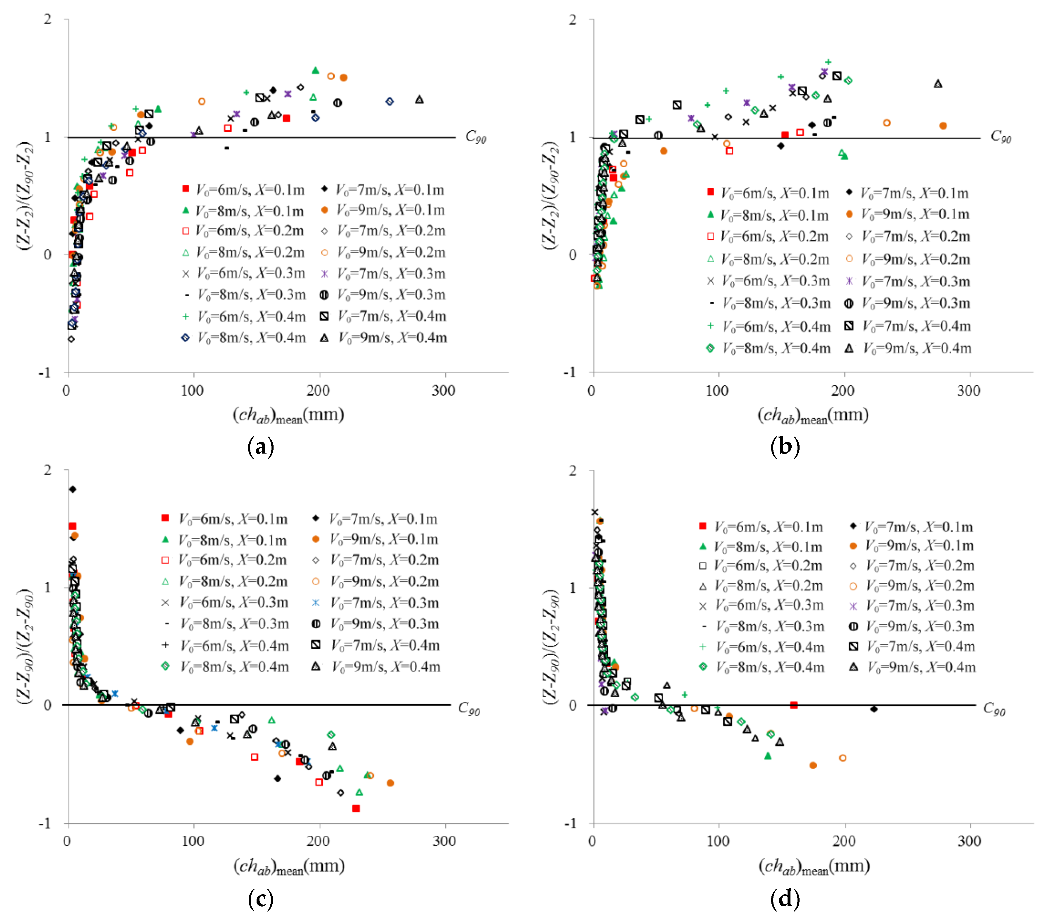

Figure 12.
Measured air bubble chord length as a function of the air concentration. The solid lines are determined from Equation (6). Upper nappe (a) (h, b) = (4.5 cm, 4.5 cm), θ = 0%. (b) (h, b) = (2.5 cm, 2.5 cm), θ = 10%; lower nappe (c) (h, b) = (4.5 cm, 4.5 cm), θ = 0%. (d) (h, b) = (2.5 cm, 2.5 cm), θ = 10%; side nappe (e) (h, b) = (4.5 cm, 4.5 cm), θ = 0%. (f) (h, b) = (2.5 cm, 2.5 cm), θ = 10%.
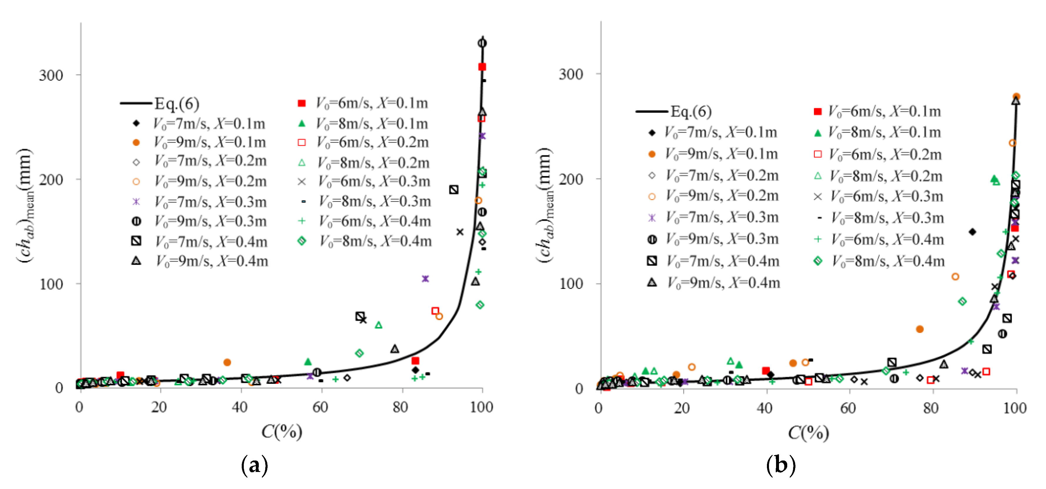

Figure 13.
Comparison of experimental data with calculated values of air bubble chord length. (a) upper nappe; (b) lower nappe; (c) side nappe.
Figure 13.
Comparison of experimental data with calculated values of air bubble chord length. (a) upper nappe; (b) lower nappe; (c) side nappe.

Figure 14.
Dimensionless bubble frequency as a function of the bubble chord length compared with the theoretical curve derived from Equation (9). Upper nappe (a) (h, b) = (4.5 cm, 4.5 cm), θ = 10%. (b) (h, b) = (6.5 cm, 6.5 cm), θ = 10%; lower nappe (c) (h, b) = (4.5 cm, 4.5 cm), θ = 10%. (d) (h, b) = (6.5 cm, 6.5 cm), θ = 10%; side nappe (e) (h, b) = (4.5 cm, 4.5 cm), θ = 10%. (f) (h, b) = (6.5 cm, 6.5 cm), θ = 10%.

Figure 15.
Comparison of experimental data with calculated values of dimensionless bubble frequency. (a) upper nappe; (b) lower nappe; (c) side nappe.
Figure 15.
Comparison of experimental data with calculated values of dimensionless bubble frequency. (a) upper nappe; (b) lower nappe; (c) side nappe.


Table 1.
Summary of the operating conditions for the experiments.
| Series | (h, b)/m | θ |
|---|---|---|
| 1 | (0.025, 0.000) | 10% |
| 2 | (0.045, 0.000) | 10% |
| 3 | (0.065, 0.000) | 10% |
| 4 | (0.000, 0.025) | 10% |
| 5 | (0.000, 0.045) | 10% |
| 6 | (0.000, 0.065) | 10% |
| 7 | (0.025, 0.025) | 10% |
| 8 | (0.045, 0.045) | 10% |
| 9 | (0.065, 0.065) | 10% |
| 10 | (0.045, 0.045) | 0% |
| 11 | (0.000, 0.045) | 0% |
| 12 | (0.045, 0.000) | 0% |
| 13 | (0.045, 0.045) | 25% |
| 14 | (0.000, 0.045) | 25% |
| 15 | (0.045, 0.000) | 25% |
Table 2.
Values of μ0 and σ0.
| Nappe | μ0 | σ0 |
|---|---|---|
| lower | 0.326 | 0.419 |
| upper | 0.210 | 0.413 |
| side | 0.283 | 0.423 |
© 2018 by the author. Licensee MDPI, Basel, Switzerland. This article is an open access article distributed under the terms and conditions of the Creative Commons Attribution (CC BY) license (http://creativecommons.org/licenses/by/4.0/).
Share and Cite
MDPI and ACS Style
Li, S.; Zhang, J.; Chen, X.; Chen, J. Three-Dimensional Aerators: Characteristics of the Air Bubbles. Water 2018, 10, 1430. https://doi.org/10.3390/w10101430
AMA Style
Li S, Zhang J, Chen X, Chen J. Three-Dimensional Aerators: Characteristics of the Air Bubbles. Water. 2018; 10(10):1430. https://doi.org/10.3390/w10101430
Chicago/Turabian StyleLi, Shuai, Jianmin Zhang, Xiaoqing Chen, and Jiangang Chen. 2018. "Three-Dimensional Aerators: Characteristics of the Air Bubbles" Water 10, no. 10: 1430. https://doi.org/10.3390/w10101430
Note that from the first issue of 2016, this journal uses article numbers instead of page numbers. See further details here.