Hydrologic Regime Changes in a High-Latitude Glacierized Watershed under Future Climate Conditions


Abstract
:1. Introduction
2. Materials and Methods
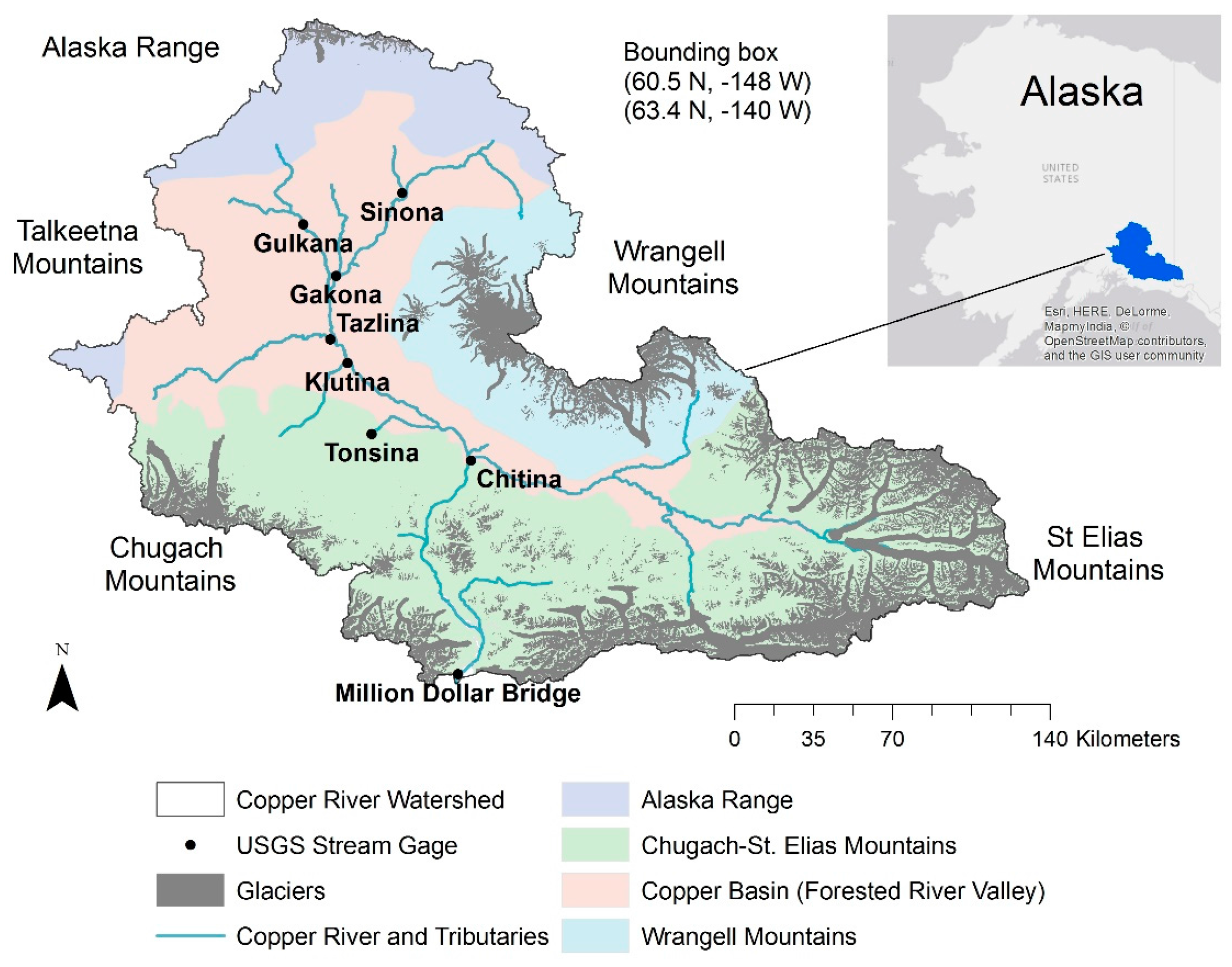
2.1. Study Area
2.2. Data
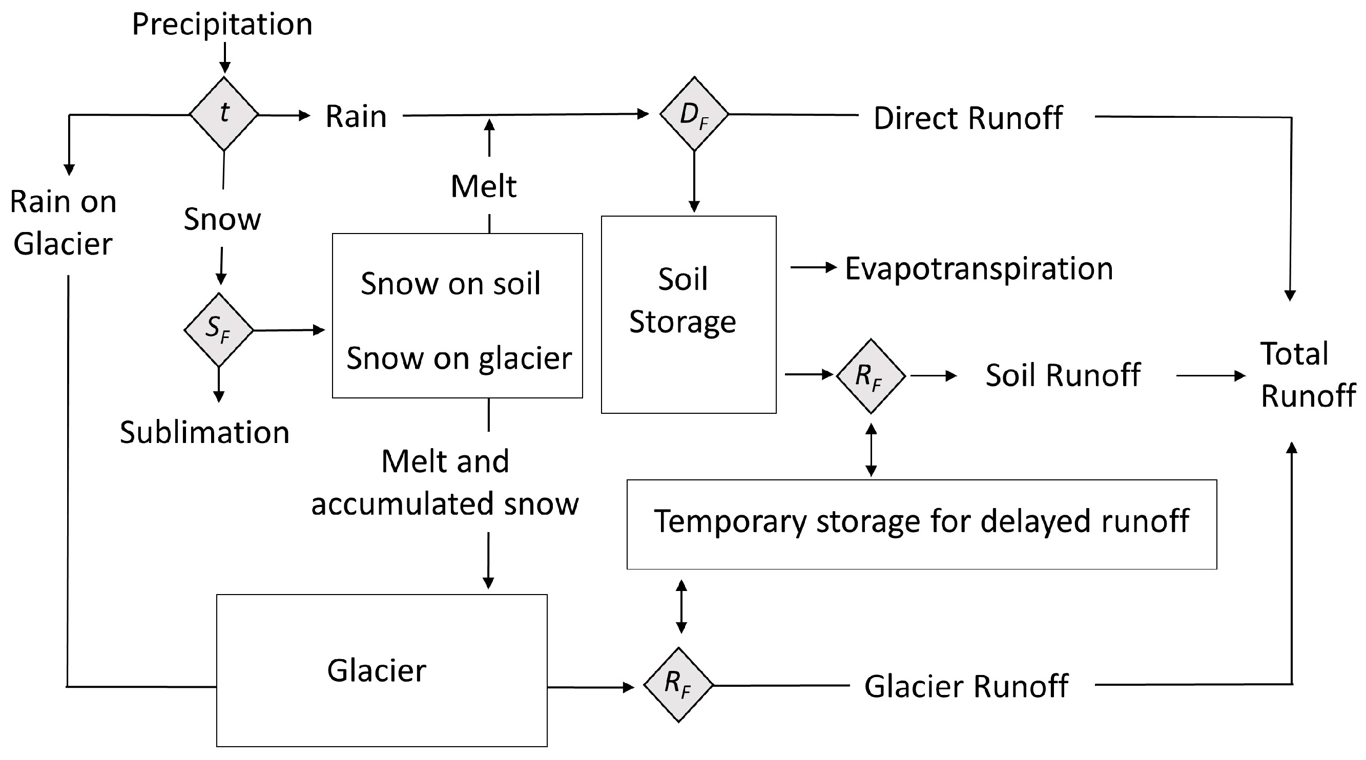
2.3. Glacio-Hydrological Modeling
Step 1: Snow and Rain Partitioning
Step 2: Snow Accumulation and Ablation
Step 3: Direct Runoff
Step 4: Evapotranspiration
Step 5: Soil Saturation Runoff
Step 6: Glacier Accumulation and Ablation
Step 7: Storage and Delayed Release of Runoff from Soil and Glaciers
Step 8: Total Runoff
Step 9: Water Balance Calculation and Model Output
- Storage in snow, glaciers, soil, and the Delay lagging reservoir,
- Precipitation partitioning into snow and rain,
- Runoff generated from rain, snowmelt, and glacier ice melt, and
- Transfers to the atmosphere in the form of sublimation and evapotranspiration.
Step 10: Change in Glacier Area
2.4. Identification of Hydrologic Regime Changes
3. Results
3.1. Glacio-Hydrological Modeling
3.1.1. Evaluation of Model Performance 2006–2016
- Streamflow calibration and evaluation was acceptable at the six stream gauges whose catchment areas included glaciers (Million Dollar, Tonsina, Klutina, Tazlina, and Gakona) with NSE ranging from 0.79 to 0.89, RSR from 0.33 to 0.45, and PBIAS from 1.4% to 29% at those gauges. Streamflow calibration was not acceptable at the two unglacierized tributaries (Gulkana and Sinona).
- Calibration of SCA to MODIS satellite-based observations (MOD10CM) was acceptable in all four ecoregions (NSE 0.89–0.93), but when the results were further evaluated by elevation band, calibration was unacceptable in the two regions where elevations exceeded 2500 m.
- Twenty-three comparisons were made between simulated mass balance change (Δmb) at 12 individual glaciers during specific time periods where data were available in the published literature (reference data). The mean Δmb for all reference data was −0.64 ± 0.36 m water equivalent per year (mwe/year) and corresponding simulated results were −0.72 ± 0.35 mwe/year.
- A comparison of monthly simulated ET versus MODIS ET resulted in NSE of 0.68 with an average annual difference of 121 mm/year, with MOD16 observations generally higher than simulated ET.
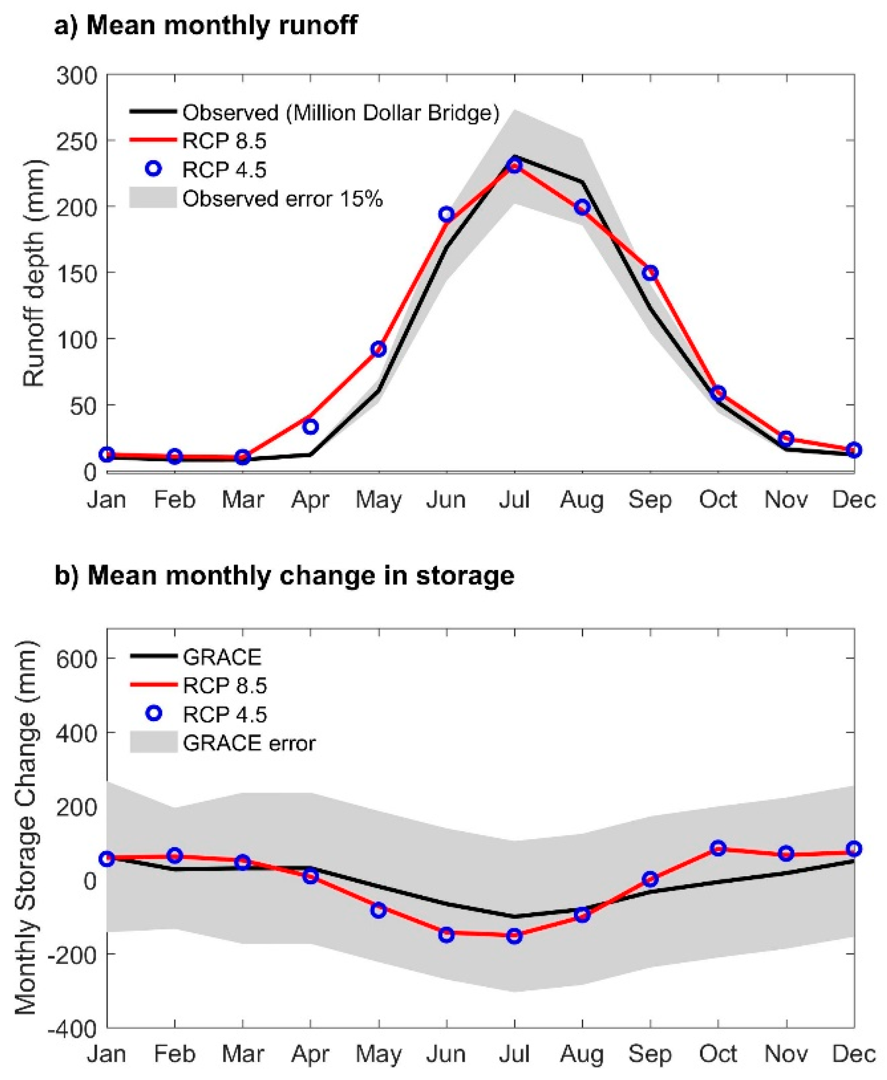
- The annual difference between GRACE and simulated ΔTWS was 50 mm or less on a monthly basis (well within the reported error associated with the GRACE data), and, on an annual basis, GRACE ΔTWS was on average 54 mm higher than simulated ΔTWS. The mean annual ΔTWS deviation represents 4% of mean annual precipitation flux.
3.1.2. Summary of Future Climate
3.1.3. Snow
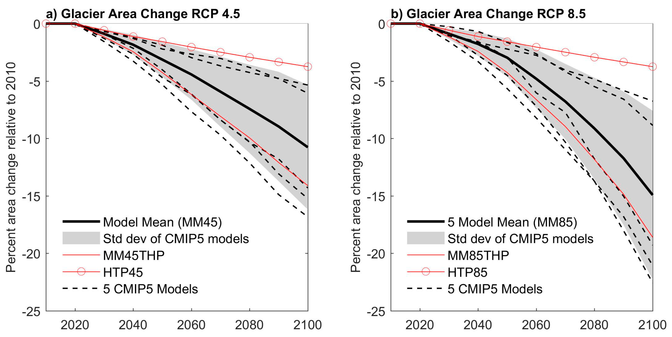
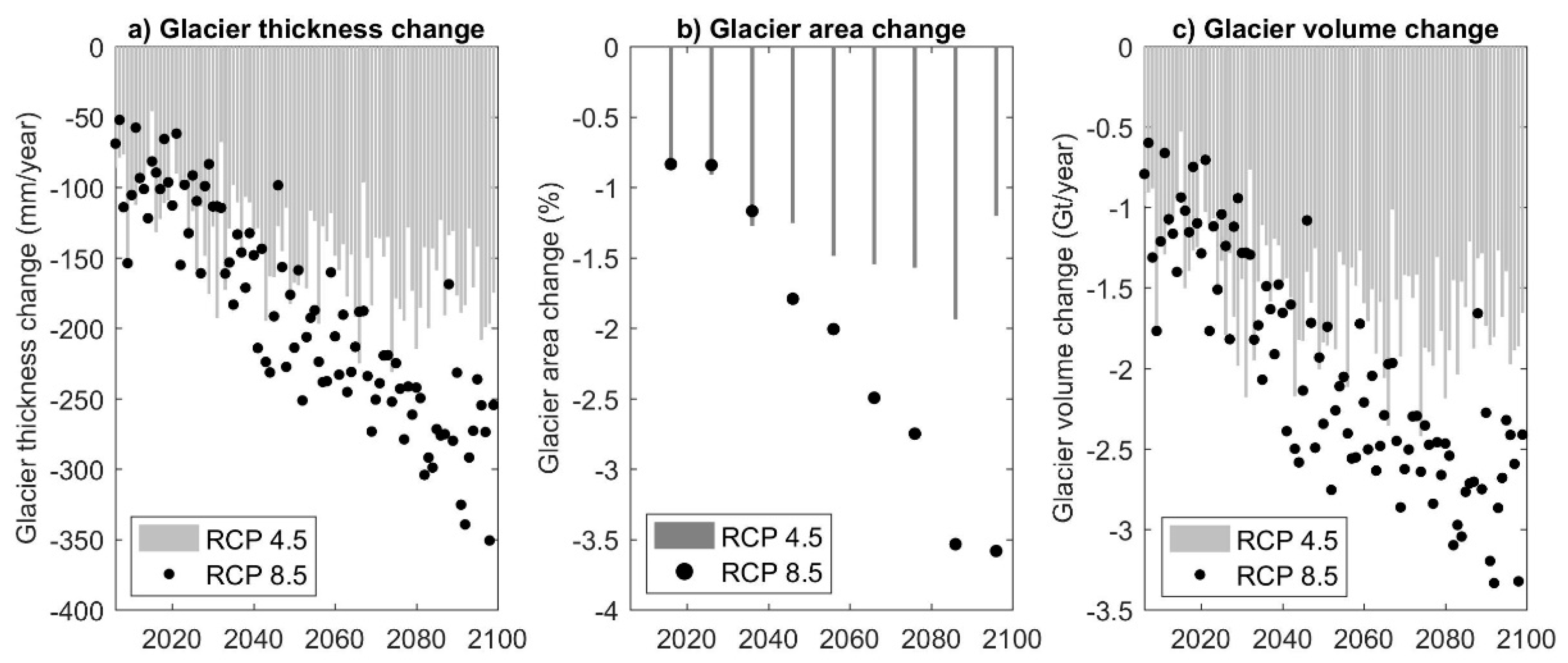
3.1.4. Glaciers
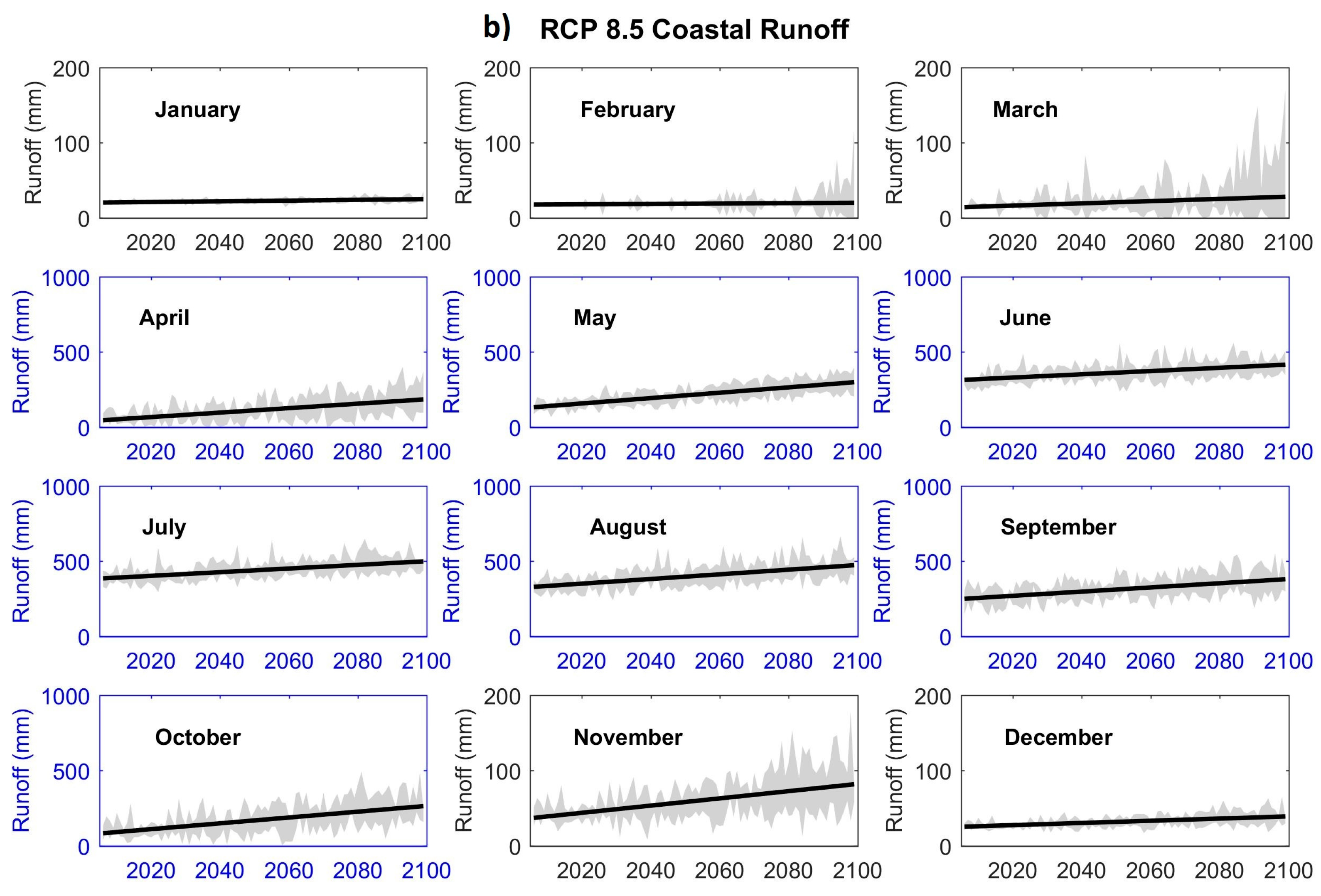
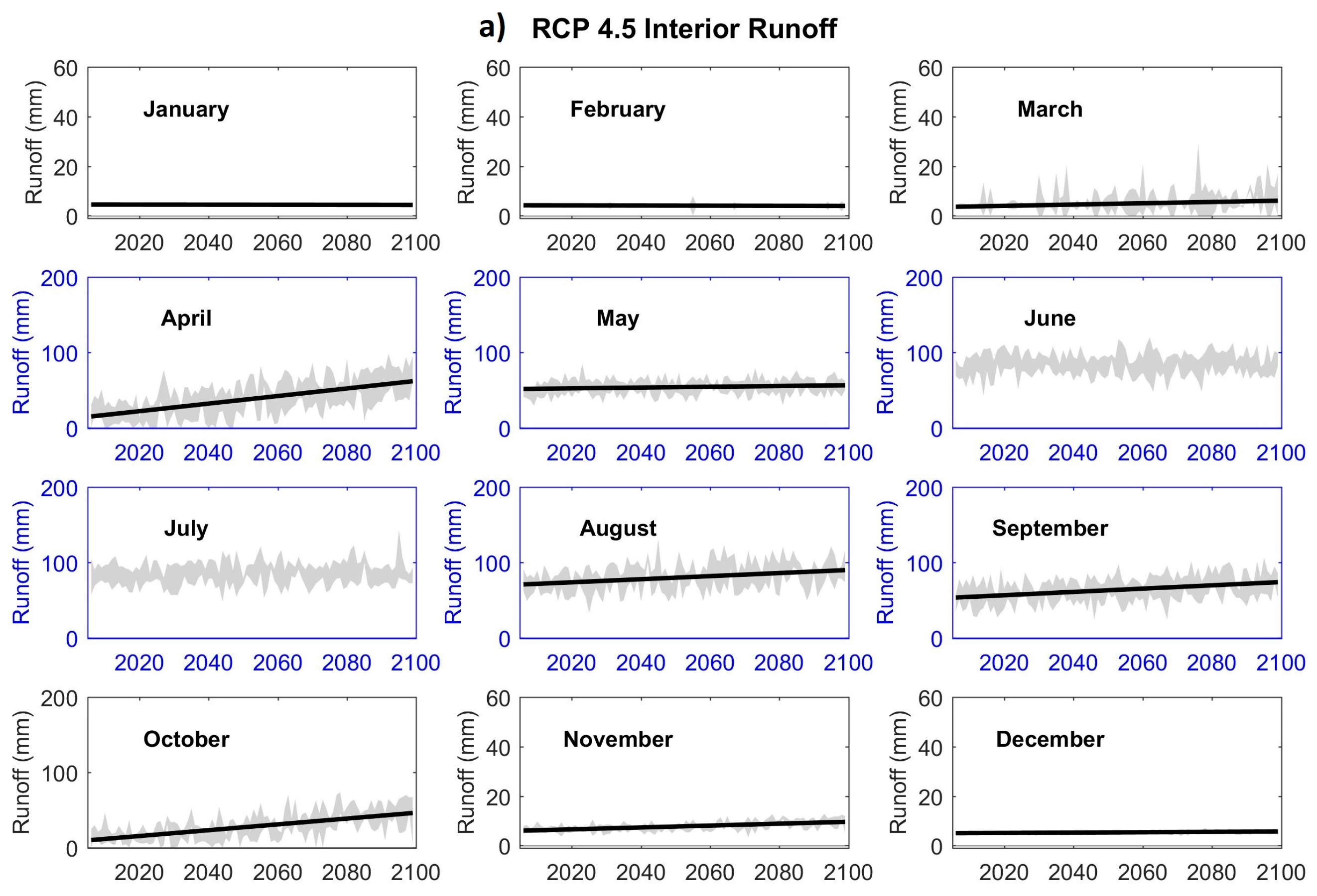
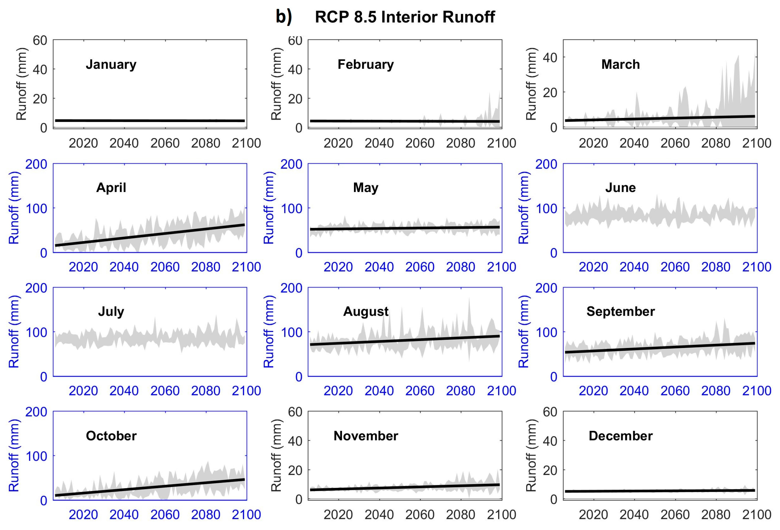
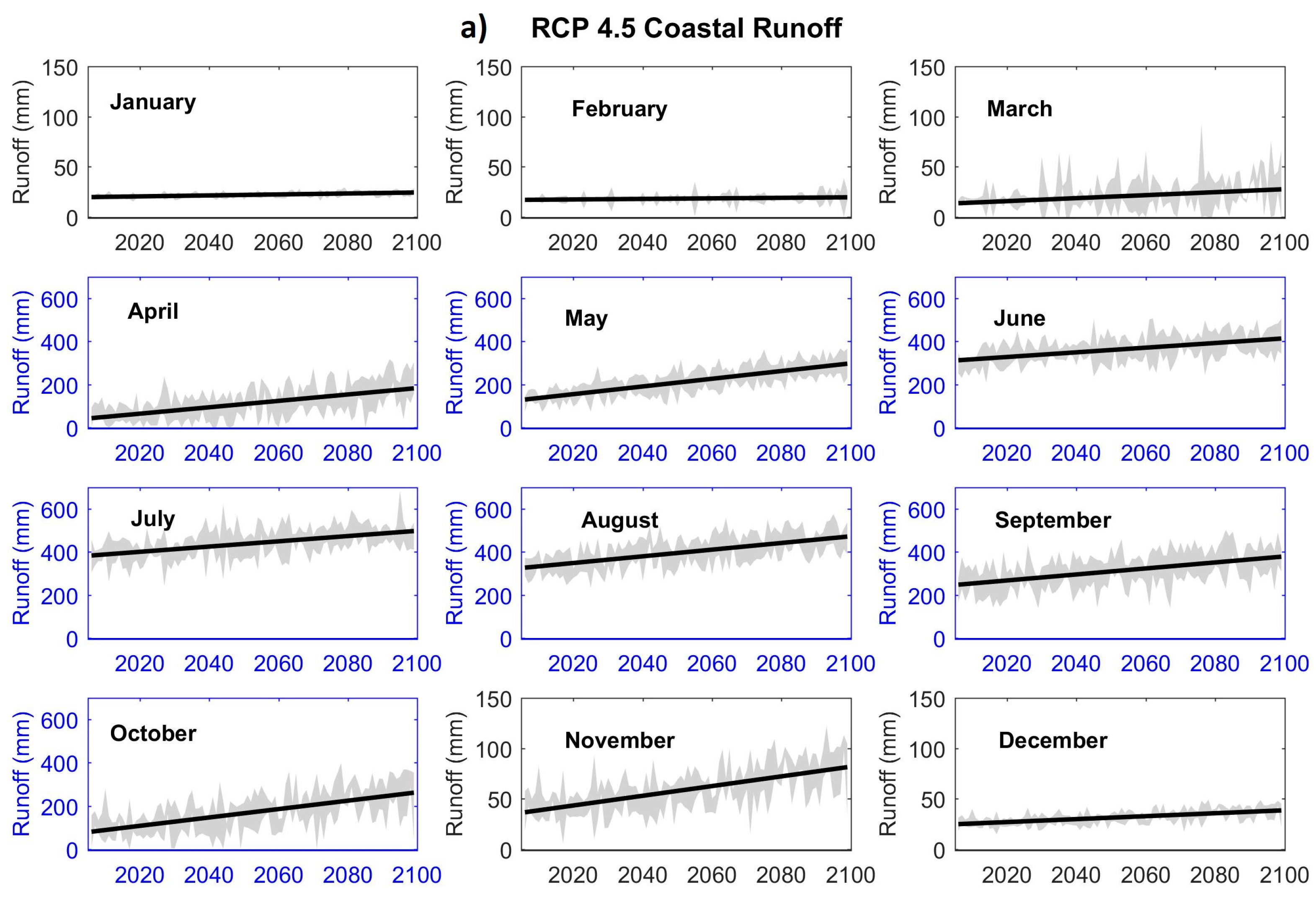
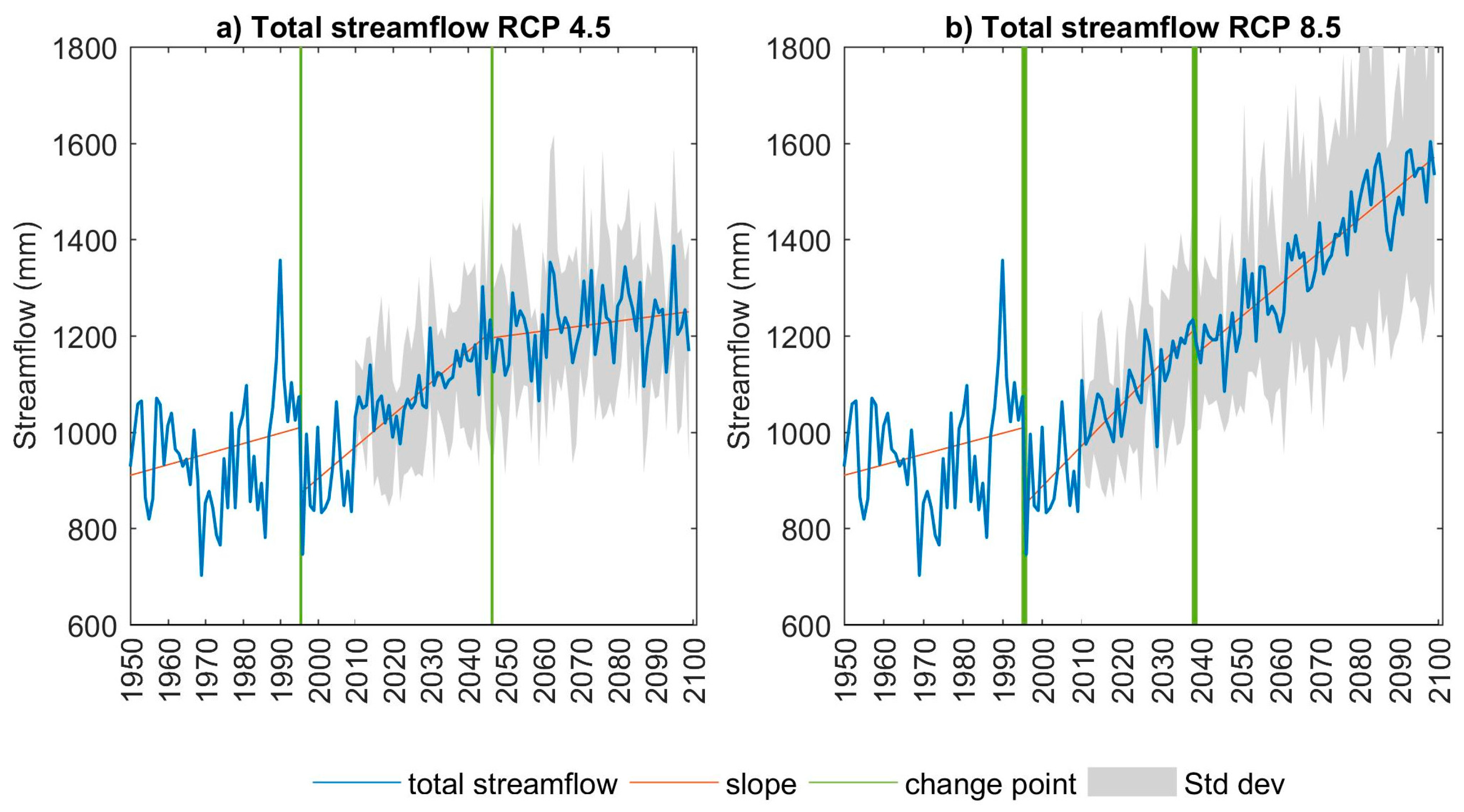
3.1.5. Future Runoff
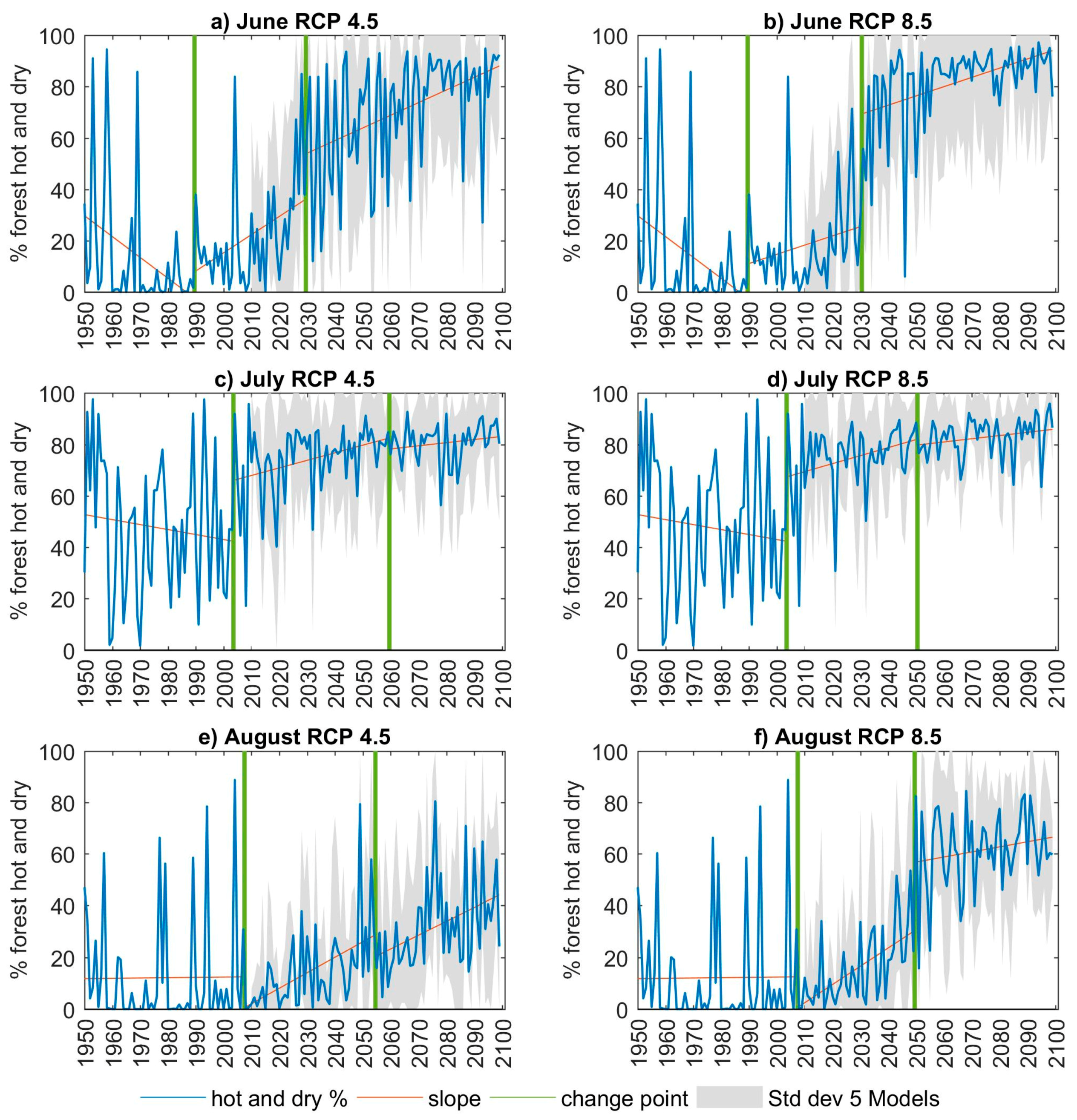
3.1.6. ET Deficit and Forest Vulnerability
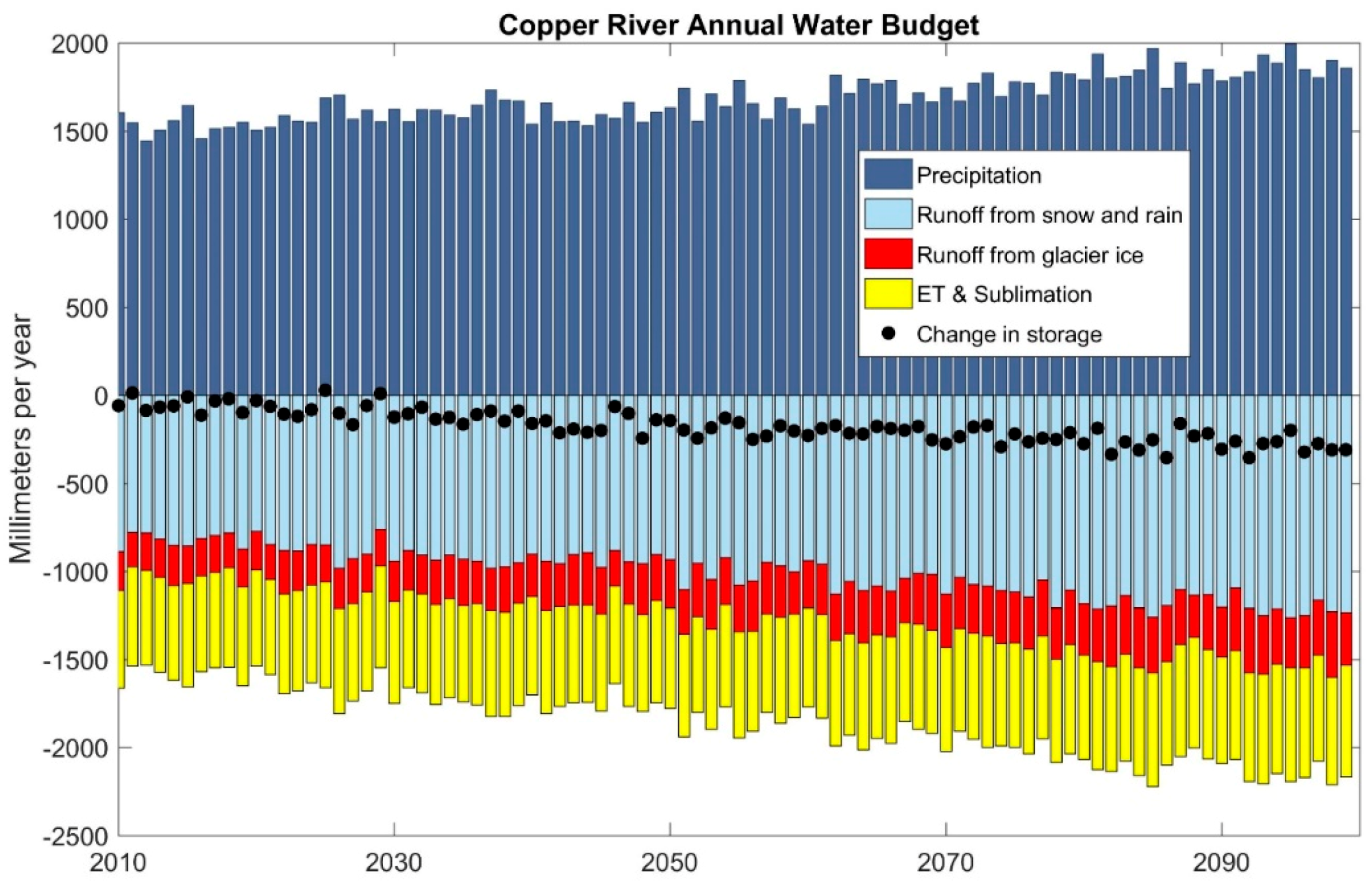
3.1.7. Water Budget
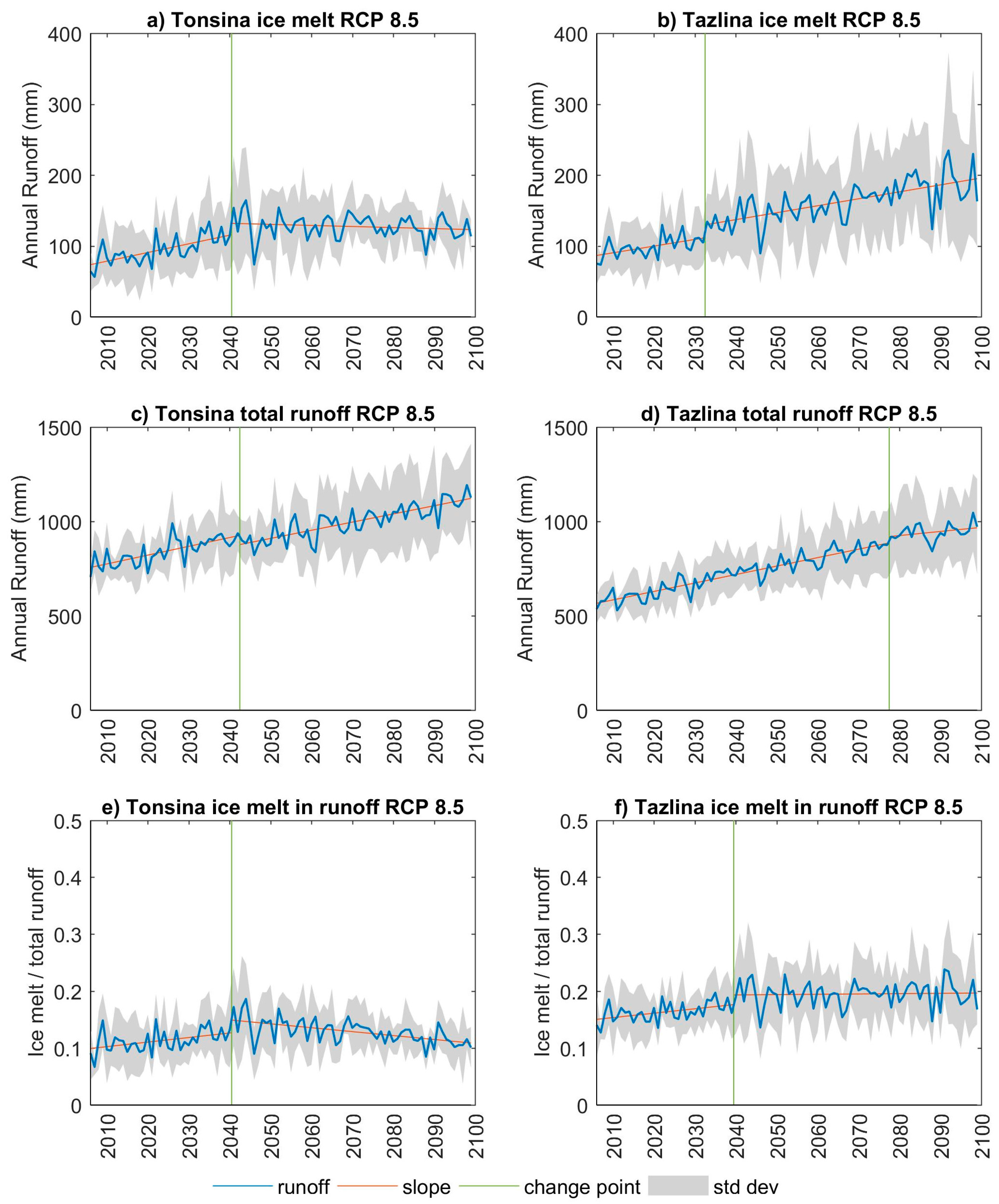
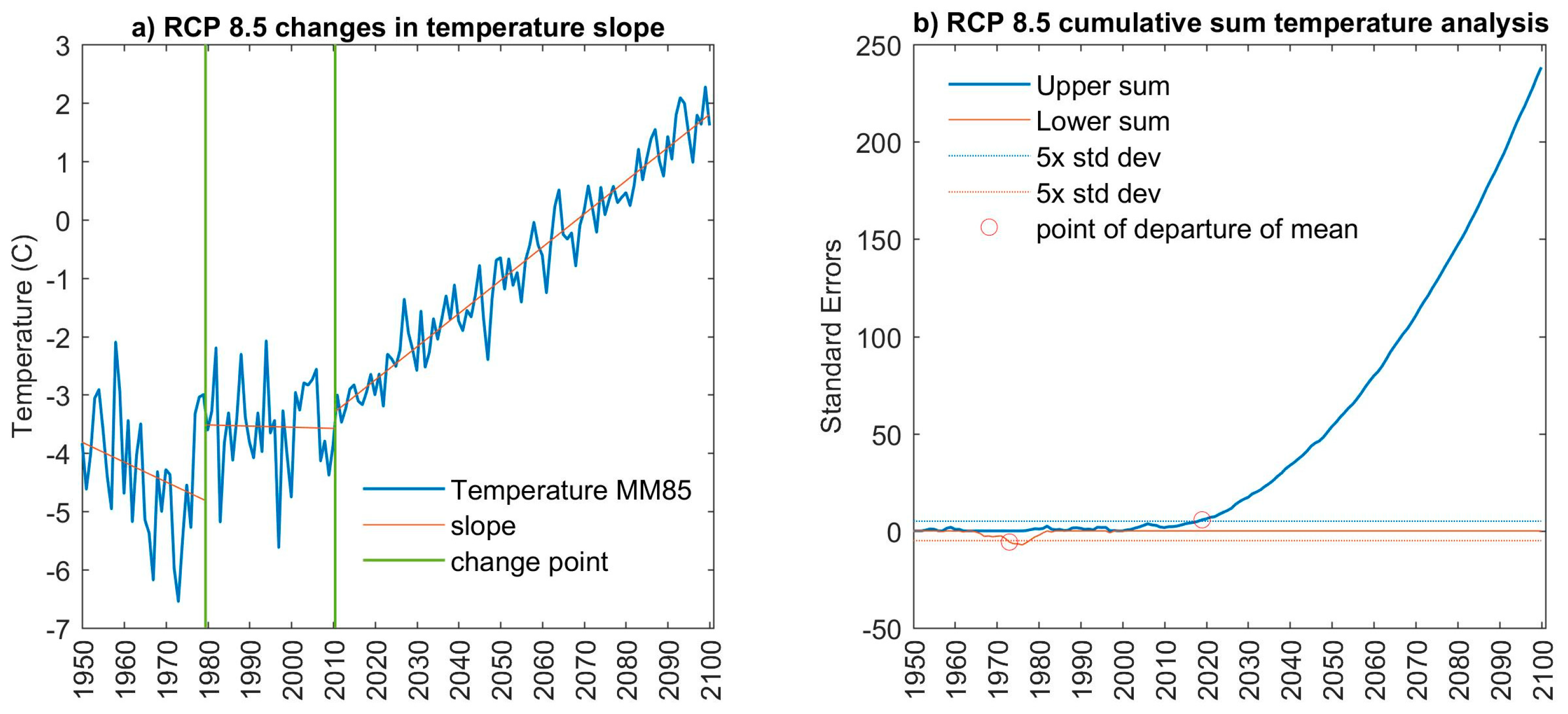
3.2. Regime Change
4. Discussion
5. Conclusions
Acknowledgments
Author Contributions
Conflicts of Interest
References
- Barnett, T.P.; Adam, J.C.; Lettenmaier, D.P. Potential impacts of a warming climate on water availability in snow-dominated regions. Nature 2005, 438, 303–309. [Google Scholar] [CrossRef] [PubMed]
- Bates, R.E.; Bilello, M.A. Defining the Cold Regions of the Northern Hemisphere; DTIC Document: Hanover, NH, USA, 1966. [Google Scholar]
- Lenton, T.M.; Held, H.; Kriegler, E.; Hall, J.W.; Lucht, W.; Rahmstorf, S.; Schellnhuber, H.J. Tipping elements in the Earth’s climate system. Proc. Natl. Acad. Sci. USA 2008, 105, 1786–1793. [Google Scholar] [CrossRef] [PubMed]
- Hagg, W.; Hoelzle, M.; Wagner, S.; Mayr, E.; Klose, Z. Glacier and runoff changes in the Rukhk catchment, upper Amu-Darya basin until 2050. Glob. Planet. Chang. 2013, 110, 62–73. [Google Scholar] [CrossRef]
- Dyurgerov, M. Mountain and subpolar glaciers show an increase in sensitivity to climate warming and intensification of the water cycle. J. Hydrol. 2003, 282, 164–176. [Google Scholar] [CrossRef]
- Radić, V.; Bliss, A.; Beedlow, A.C.; Hock, R.; Miles, E.; Cogley, J.G. Regional and global projections of twenty-first century glacier mass changes in response to climate scenarios from global climate models. Clim. Dyn. 2014, 42, 37–58. [Google Scholar] [CrossRef]
- Shugar, D.H.; Clague, J.J.; Best, J.L.; Schoof, C.; Willis, M.J.; Copland, L.; Roe, G.H. River piracy and drainage basin reorganization led by climate-driven glacier retreat. Nat. Geosci. 2017, 10, 370–375. [Google Scholar] [CrossRef]
- Arendt, A.A.; Echelmeyer, K.A.; Harrison, W.D.; Lingle, C.S.; Valentine, V.B. Rapid wastage of Alaska glaciers and their contribution to rising sea level. Science 2002, 297, 382–386. [Google Scholar] [CrossRef] [PubMed]
- Stewart, I.T.; Ficklin, D.L.; Carrillo, C.A.; McIntosh, R. 21st century increases in the likelihood of extreme hydrologic conditions for the mountainous basins of the Southwestern United States. J. Hydrol. 2015, 529, 340–353. [Google Scholar] [CrossRef]
- Walvoord, M.A.; Kurylyk, B.L. Hydrologic impacts of thawing permafrost—A review. Vadose Zone J. 2016, 15. [Google Scholar] [CrossRef]
- Walvoord, M.A.; Striegl, R.G. Increased groundwater to stream discharge from permafrost thawing in the Yukon River basin: Potential impacts on lateral export of carbon and nitrogen. Geophys. Res. Lett. 2007, 34. [Google Scholar] [CrossRef]
- Young, A.M.; Higuera, P.E.; Duffy, P.A.; Hu, F.S. Climatic thresholds shape northern high-latitude fire regimes and imply vulnerability to future climate change. Ecography 2017, 40, 606–617. [Google Scholar] [CrossRef]
- Jorgenson, M.; Yoshikawa, K.; Kanevskiy, M.; Shur, Y.; Romanovsky, V.; Marchenko, S.; Grosse, G.; Brown, J.; Jones, B. Permafrost characteristics of Alaska. In Proceedings of the Ninth International Conference on Permafrost, Fairbanks, AK, USA, 28 June–3 July 2008; pp. 121–122. [Google Scholar]
- Poff, N.L.; Zimmerman, J.K. Ecological responses to altered flow regimes: a literature review to inform the science and management of environmental flows. Freshw. Biol. 2010, 55, 194–205. [Google Scholar] [CrossRef]
- Nowacki, G.J.; Spencer, P.; Fleming, M.; Brock, T.; Jorgenson, T. Unified Ecoregions of Alaska: 2001; U.S. Geological Survey: Reston, VA, USA, 2003; ISBN 0607995777.
- Brabets, T.; Conaway, J. Geomorphology and River Dynamics of the Lower Copper River, Alaska; U.S. Geological Survey: Reston, VA, USA, 2009.
- Van Vuuren, D.P.; Edmonds, J.; Kainuma, M.; Riahi, K.; Thomson, A.; Hibbard, K.; Hurtt, G.C.; Kram, T.; Krey, V.; Lamarque, J.-F. The representative concentration pathways: An overview. Clim. Chang. 2011, 109, 5. [Google Scholar] [CrossRef]
- Saha, S.; Moorthi, S.; Pan, H.L.; Wu, X.R.; Wang, J.D.; Nadiga, S.; Tripp, P.; Kistler, R.; Woollen, J.; Behringer, D.; et al. The Ncep Climate Forecast System Reanalysis. Bull. Am. Meteorol. Soc. 2010, 91, 1015–1057. [Google Scholar] [CrossRef]
- Valiantzas, J.D. Simplified versions for the Penman evaporation equation using routine weather data. J. Hydrol. 2006, 331, 690–702. [Google Scholar] [CrossRef]
- Valiantzas, J.D. Simplified forms for the standardized FAO-56 Penman–Monteith reference evapotranspiration using limited weather data. J. Hydrol. 2013, 505, 13–23. [Google Scholar] [CrossRef]
- Pastick, N.J.; Jorgenson, M.T.; Wylie, B.K.; Nield, S.J.; Johnson, K.D.; Finley, A.O. Distribution of near-surface permafrost in Alaska: estimates of present and future conditions. Remote Sens. Environ. 2015, 168, 301–315. [Google Scholar] [CrossRef]
- Pfeffer, W.T.; Arendt, A.A.; Bliss, A.; Bolch, T.; Cogley, J.G.; Gardner, A.S.; Hagen, J.-O.; Hock, R.; Kaser, G.; Kienholz, C.; et al. The Randolph Glacier Inventory: a globally complete inventory of glaciers. J. Glaciol. 2014, 60, 537–552. [Google Scholar] [CrossRef] [Green Version]
- Riggs, G.A.; Hall, D.K.; Salomonson, V.V. MODIS snow products user guide to collection 5. Digit. Media 2006, 80, 1–80. [Google Scholar]
- Mu, Q.; Zhao, M.; Running, S.W. Improvements to a MODIS global terrestrial evapotranspiration algorithm. Remote Sens. Environ. 2011, 115, 1781–1800. [Google Scholar] [CrossRef]
- Taylor, K.E.; Stouffer, R.J.; Meehl, G.A. An overview of CMIP5 and the experiment design. Bull. Am. Meteorol. Soc. 2012, 93, 485–498. [Google Scholar] [CrossRef]
- Walsh, J.E.; Chapman, W.L.; Romanovsky, V.; Christensen, J.H.; Stendel, M. Global climate model performance over Alaska and Greenland. J. Clim. 2008, 21, 6156–6174. [Google Scholar] [CrossRef]
- Wood, A.W.; Leung, L.R.; Sridhar, V.; Lettenmaier, D. Hydrologic implications of dynamical and statistical approaches to downscaling climate model outputs. Clim. Chang. 2004, 62, 189–216. [Google Scholar] [CrossRef]
- Hay, L.E.; Wilby, R.L.; Leavesley, G.H. A comparison of delta change and downscaled GCM scenarios for three mountainous basins in the United States. J. Am. Water Resour. Assoc. 2000, 36, 387–397. [Google Scholar] [CrossRef]
- Valentin, M.M.; Viger, R.J.; Van Beusekom, A.E.; Hay, L.E.; Hogue, T.S.; Foks, N.L. Identifying Climate-Related Hydrologic Regime Change in Mountainous Cold-Region Watersheds. Ph.D. Dissertation, Colorado School of Mines, Golden, CO, USA, 2017; pp. 40–63. [Google Scholar]
- Brock, T.D. Calculating solar radiation for ecological studies. Ecol. Modell. 1981, 14, 1–19. [Google Scholar] [CrossRef]
- Braithwaite, R.; Raper, S. Estimating equilibrium-line altitude (ELA) from glacier inventory data. Ann. Glaciol. 2010, 50, 127–132. [Google Scholar] [CrossRef]
- Bahr, D.B.; Pfeffer, W.T.; Kaser, G. A review of volume-area scaling of glaciers. Rev. Geophys. 2015, 53, 95–140. [Google Scholar] [CrossRef] [PubMed]
- Raper, S.C.; Braithwaite, R.J. Glacier volume response time and its links to climate and topography based on a conceptual model of glacier hypsometry. Cryosphere 2009, 3, 183–194. [Google Scholar] [CrossRef]
- Bahr, D.B.; Meier, M.F.; Peckham, S.D. The physical basis of glacier volume-area scaling. J. Geophys. Res. Solid Earth 1997, 102, 20355–20362. [Google Scholar] [CrossRef]
- Dakos, V.; Carpenter, S.R.; Brock, W.A.; Ellison, A.M.; Guttal, V.; Ives, A.R.; Kefi, S.; Livina, V.; Seekell, D.A.; van Nes, E.H. Methods for detecting early warnings of critical transitions in time series illustrated using simulated ecological data. PLoS One 2012, 7, e41010. [Google Scholar] [CrossRef] [PubMed] [Green Version]
- Killick, R.; Fearnhead, P.; Eckley, I.A. Optimal detection of changepoints with a linear computational cost. J. Am. Stat. Assoc. 2012, 107, 1590–1598. [Google Scholar] [CrossRef]
- Montgomery, D.C. Statistical Quality Control; Wiley: New York, NY, USA, 2009; Volume 7. [Google Scholar]
- Gibbons, J.D.; Chakraborti, S. Nonparametric Statistical Inference; Springer: Berlin/Heidelberg, Germany, 2011. [Google Scholar]
- Bliss, A.; Hock, R.; Radic, V. Global response of glacier runoff to twenty-first century climate change. J. Geophys. Res.-Earth Surf. 2014, 119, 717–730. [Google Scholar] [CrossRef]
- Valentin, M.M.; Hay, L.E.; Hogue, T.S. Model Input and Output Data for Historical and Potential Future Hydrologic Simulations in the Copper River Basin in Alaska Using the Monthly Water Balance Model Adapted for Use in Glacierized Watersheds (MWBMglacier). Ph.D. Thesis, Colorado School of Mines, Golden, CO, USA, 2017. [Google Scholar]
- Moriasi, D.N.; Arnold, J.G.; Van Liew, M.W.; Bingner, R.L.; Harmel, R.D.; Veith, T.L. Model evaluation guidelines for systematic quantification of accuracy in watershed simulations. Trans. ASABE 2007, 50, 885–900. [Google Scholar] [CrossRef]
- Larsen, C.; Burgess, E.; Arendt, A.; O’Neel, S.; Johnson, A.; Kienholz, C. Surface melt dominates Alaska glacier mass balance. Geophys. Res. Lett. 2015, 42, 5902–5908. [Google Scholar] [CrossRef]
- Das, I.; Hock, R.; Berthier, E.; Lingle, C.S. 21st-century increase in glacier mass loss in the Wrangell Mountains, Alaska, USA, from airborne laser altimetry and satellite stereo imagery. J. Glaciol. 2014, 60, 283–293. [Google Scholar] [CrossRef] [Green Version]
- Merritt, M.; Roberson, K. Migratory timing of upper Copper River sockeye salmon stocks and its implications for the regulation of the commercial fishery. N. Am. J. Fish. Manag. 1986, 6, 216–225. [Google Scholar] [CrossRef]
- Bieniek, P.A.; Walsh, J.E.; Thoman, R.L.; Bhatt, U.S. Using climate divisions to analyze variations and trends in Alaska temperature and precipitation. J. Clim. 2014, 27, 2800–2818. [Google Scholar] [CrossRef]
- Kim, H.M.; Webster, P.J.; Curry, J.A. Evaluation of short-term climate change prediction in multi-model CMIP5 decadal hindcasts. Geophys. Res. Lett. 2012, 39, 1–7. [Google Scholar] [CrossRef]
- Hock, R.; Jansson, P.; Braun, L.N. Modelling the response of mountain glacier discharge to climate warming. In Global Change and Mountain Regions; Springer: Dordrecht, The Netherlands, 2005; pp. 243–252. [Google Scholar]


| Information | Use | Source |
|---|---|---|
| Ecoregions | Model setup | Alaska ecoregion mapping [15] accessed 27 November 2016 (https://agdc.usgs.gov/data/usgs/erosafo/ecoreg/). |
| Monthly Temperature and Precipitation | Model input | Scenarios Network for Alaska and Arctic Planning (SNAP) accessed February 2016 and April 2017. Temperature and precipitation data for years 2006 through 2099 at 2 km resolution was obtained for the following 5 CMIP5 models NCAR-CCSM4, CGDF-CM3, GISS-ER-2, IPSL-CM5A-LR, MRI-CGCM3, and five-model means, for two scenarios: RCP 4.5 and RCP 8.5. Historical data was used for calibration and evaluation at the same 2 km resolution, 1949 to 2009 (https://www.snap.uaf.edu/). |
| Supplemental climate data | Hamon coefficient calibration | Climate Forecast Reanalysis Data (CFSR) gridded climate variables [18] at ~38 km spatial resolution, 1979–2013 (https://globalweather.tamu.edu) accessed 19 May 2016 for Penman Monteith PET calculation [19,20] |
| Permafrost probability | Model setup | Permafrost mapping for Alaska [21] accessed 2 August 2016 (https://dx.doi.org/10.5066/F7C53HX6). |
| Glacierized area in 2010 | Model setup | Randolph Glacier Inventory 5.0 [22] accessed 11 March 2016 (http://www.glims.org/RGI/). |
| Elevation | Model setup | Alaska Division of Geologic and Geophysical Surveys accessed March 2013 (http://maps.dggs.alaska.gov/elevationdata/). |
| Soil water holding capacity | Model Setup | U.S. Department of Agriculture, accessed March 2013 (https://www.nrcs.usda.gov/wps/portal/nrcs/main/ak/soils/surveys/). |
| Snow Covered Area | Model calibration | MODIS Monthly Snow Covered Area MOD10CM. [23] accessed 27 August 2016 (https://nsidc.org/data/mod10cm). |
| Streamflow | Model calibration | USGS National Water Information System, accessed 29 January 2016 (https://waterdata.usgs.gov/usa/nwis/). Data uncertainty may exceed 15% (https://wdr.water.usgs.gov/current/documentation.html accessed 8 June 2017). |
| GRACE observations of change in storage | Model evaluation | University of Colorado GRACE Data Analysis Website, GRACE Release 05 Level 2 data processed by the Center for Space Research (CSR), the German Research Centre for Geosciences (GFZ), and the Jet Propulsion Laboratory (JPL). Accessed 21 May 2017 (http://geoid.colorado.edu/grace/). |
| Evapo-transpiration | Model evaluation | MOD16 monthly evapotranspiration and potential evapotranspiration, (http://www.ntsg.umt.edu/project/mod16) [24] accessed 24 May 2017 on the Geo Data Portal (https://cida.usgs.gov/gdp). |
| Meteorological variables for PET | Model setup | Climate Forecast Reanalysis System (CFSR) gridded meteorological data [18] accessed through the Texas A&M website, Global weather data for SWAT, 22 May 2016 (https://globalweather.tamu.edu/). |
| Forested area | Model setup | US Forest Service, orest Inventory and Analysis Program and Remote Sensing Applications Center, ArcGIS Online, accessed 28 October 2016. |
| Climate Data Source | Scenario and Simulation Code |
|---|---|
| 1. Historical climate | 1949–2009 (HISTOBS) |
| 2. CMIP5 CCSM4 | RCP 4.5 (CC45) and RCP 8.5 (CC85) |
| 3. CMIP5 GFDL | RCP 4.5 (GF45) and RCP 8.5 (GF85) |
| 4. CMIP5 GISS | RCP 4.5 (GI45) and RCP 8.5 (GI85) |
| 5. CMIP5 IPSL | RCP 4.5 (IP45) and RCP 8.5 (IP85) |
| 6. CMIP5 MRI | RCP 4.5 (MR45) and RCP 8.5 (MR85) |
| 7. CMIP5 5-Model Mean | RCP 4.5 (MM45) and RCP 8.5 (MM85) |
| 8. Historical Mean Monthly | 1949–2009 mean monthly repeated for 2006 through 2099 (HTP) |
| 9. Historical precipitation with future temperature | RCP 4.5 (MM45THP) and RCP 8.5 (MM85THP) |
| 10. Temperature sensitivity analysis | The historical temperature record, 1949–2009, was increased by 2, 4, 6, 8, and 10 degrees C (corresponding to scenarios S2, S4, S6, S8, and S10, respectively). The historical precipitation record was unaltered. |
| Parameters | Description and Recommended Range of Values |
| TSNOW | Snow temperature (°C), range −10 °C to +5 °C, default −0.72 °C |
| TRAIN | Rain temperature (°C), range −5 °C to +10 °C, default 3.71 °C |
| TMELT | Melt temperature (°C), recommended range −5 °C to +5 °C, default 0.97 °C |
| RFAC | Runoff factor, range 0 to 1, default 0.50 |
| DROFAC | Direct runoff factor, range 0 to 1, default 0.01 |
| SMELTR | Rate of snow melt (mm/°C /day), minimum 0, default 4.83 |
| GMELTR | Rate of exposed ice melt (mm/°C /day), minimum 0, default 5.0 |
| GBFLOW | Glacier base flow (mm/month), minimum 0, default 50. |
| SUBFAC | Fraction of snowfall that sublimates, range 0 to 1, default 0.06 |
| HC | Monthly Hamon coefficient (dimensionless), minimum 0, default 0.55 |
| Input Data | Description |
| MRUs | Spatial representation of the watershed |
| Precipitation | Monthly precipitation time series (mm) for each MRU |
| Temperature | Monthly temperature time series (°C) for each MRU |
| Latitude | MRU latitude in decimal degrees |
| AWC | MRU available soil water content (mm) |
| Land type | Glacier, permafrost, or permeable soil |
| Area | MRU area (km2) |
| Elevation | MRU elevation (m) |
| Water Cycle Components | RCP 4.5 Decadal Means (mm/Year) | RCP 8.5 Decadal Means (mm/Year) | ||||
|---|---|---|---|---|---|---|
| 2010–2019 | 2050–2059 | 2090–2099 | 2010–2019 | 2050–2059 | 2090–2099 | |
| Precipitation | 1545 ± 82 | 1643 ± 105 | 1655 ± 104 | 1535 ± 100 | 1661 ± 71 | 1864 ± 166 |
| Snowfall | 887 ± 63 | 897 ± 60 | 856 ± 24 | 901 ± 46 | 856 ± 20 | 859 ± 87 |
| Rainfall | 659 ± 53 | 745 ± 78 | 799 ± 112 | 634 ± 74 | 805 ± 70 | 1005 ± 186 |
| ET & sublimation | 553 ± 22 | 576 ± 26 | 578 ± 27 | 554 ± 18 | 577 ± 19 | 621 ± 42 |
| Total runoff | 1056 ± 73 | 1183 ± 106 | 1236 ± 150 | 1036 ± 79 | 1278 ± 131 | 1535 ± 246 |
| Glacier ice melt | 217 ± 26 | 240 ± 40 | 245 ± 38 | 212 ± 25 | 278 ± 42 | 324 ± 86 |
| Decade | Description of Regime Change for RCP 8.5, 5-Model Mean |
|---|---|
| 1970s | A 30-year period of increasingly cool temperatures associated with the Pacific Decadal Oscillation (PDO) transitions to a 30-year warm PDO warm phase. |
| 1980s | Glacier AAR begins to decline. |
| 2010s | April snow covered area in the Wrangell, Chugach and St Elias Mountains peaks in the 2010s near 30% then begins a long, steady, decline ending the century near 10%. |
| 2020s | In the mid-2020s, hot and dry forests conditions become prevalent in the month of June. |
| 2040s | In the 2040s, glacier ice contributions to streamflow in the Tonsina River stops accelerating and begins to decline due to loss of critical glacier mass |
| 2050s | The month of peak runoff in the Alaska Range becomes erratic, changing from June to May–August, and expanding to April–September in the 2090s. |
| 2050s | In the 2050s, hot and dry forest conditions become prevalent in the month of August. |
| Temperature Scenario (1960–2009) | Mann Kendall p-Value | Ice Melt Annual Trend (mm/Year/Year) | Mean Annual Ice Melt (mm/Year) |
|---|---|---|---|
| Historical (unaltered) | 0.0193 | 0.57 | 225 |
| Historical plus 2 C | 0.9095 | 0.02 | 287 |
| Historical plus 4 C | 0.0058 | −1.20 | 367 |
| Historical plus 6 C | 6.04 × 10⁻⁹ | −3.26 | 458 |
| Historical plus 8 C | 2.67 × 10⁻¹³ | −5.93 | 542 |
| Historical plus 10 C | 2.22 × 10⁻¹⁶ | −9.11 | 612 |
© 2018 by the authors. Licensee MDPI, Basel, Switzerland. This article is an open access article distributed under the terms and conditions of the Creative Commons Attribution (CC BY) license (http://creativecommons.org/licenses/by/4.0/).
Share and Cite
Valentin, M.M.; Hogue, T.S.; Hay, L.E. Hydrologic Regime Changes in a High-Latitude Glacierized Watershed under Future Climate Conditions. Water 2018, 10, 128. https://doi.org/10.3390/w10020128
Valentin MM, Hogue TS, Hay LE. Hydrologic Regime Changes in a High-Latitude Glacierized Watershed under Future Climate Conditions. Water. 2018; 10(2):128. https://doi.org/10.3390/w10020128
Chicago/Turabian StyleValentin, Melissa M., Terri S. Hogue, and Lauren E. Hay. 2018. "Hydrologic Regime Changes in a High-Latitude Glacierized Watershed under Future Climate Conditions" Water 10, no. 2: 128. https://doi.org/10.3390/w10020128
APA StyleValentin, M. M., Hogue, T. S., & Hay, L. E. (2018). Hydrologic Regime Changes in a High-Latitude Glacierized Watershed under Future Climate Conditions. Water, 10(2), 128. https://doi.org/10.3390/w10020128