Identification of Phytoplankton Blooms under the Index of Inherent Optical Properties (IOP Index) in Optically Complex Waters

Abstract

Phytoplankton blooms are sporadic events in time and are isolated in space. This complex phenomenon is produced by a variety of both natural and anthropogenic causes. Early detection of this phenomenon, as well as the classification of a water body under conditions of bloom or non-bloom, remains an unresolved problem. This research proposes the use of Inherent Optical Properties (IOPs) in optically complex waters to detect the bloom or non-bloom state of the phytoplankton community. An IOP index is calculated from the absorption coefficients of the colored dissolved organic matter (CDOM), the phytoplankton ($\mathrm{phy}$) and the detritus (d), using the wavelength (λ) 443 nm. The effectiveness of this index is tested in five bloom events in different places and with different characteristics from Mexican seas: 1. Dzilam (Caribbean Sea, Atlantic Ocean), a diatom bloom (Rhizosolenia hebetata); 2. Holbox (Caribbean Sea, Atlantic Ocean), a mixed bloom of dinoflagellates (Scrippsiella sp.) and diatoms (Chaetoceros sp.); 3. Campeche Bay in the Gulf of Mexico (Atlantic Ocean), a bloom of dinoflagellates (Karenia brevis); 4. Upper Gulf of California (UGC) (Pacific Ocean), a diatom bloom (Coscinodiscus and Pseudo-nitzschia) and 5. Todos Santos Bay, Ensenada (Pacific Ocean), a dinoflagellate bloom (Lingulodinium polyedrum). The diversity of sites show that the IOP index is a suitable method to determine the phytoplankton bloom conditions.

1. Introduction

Phytoplankton blooms are sporadic events in time and are isolated in space [1]. These complex phenomena are produced by a variety of both natural and anthropogenic causes [2]. The availability of light and nutrients is a key factor for their development [3]. This factor is illustrated during the spring summer period. At the beginning of this period, the seasonal increase in daily irradiation eliminates the light limitation, and the end of the thermal stratification provides a supply of nutrients thanks to the turbulent and convective mixing processes, which allows the phytoplankton to proliferate [4]. However, phytoplankton blooms are not only limited to this period.

Bloom is the rapid growth of one or more species leading to an increase in the species’ biomass [5]. Different adjectives have been used to characterize the degree of negative impact of these blooms according to their characteristics and those of the causative species, such as toxic, noxious or harmful [6].

Identifying phytoplankton blooms has been the target of extensive research [7,8,9,10]. Some studies have focused on detecting changes in chlorophyll a fluorescence, changes in the composition of phytoplankton species [9], or increases in nutrient levels [11]. Measurements of the intensity of blooms have also been of great interest, including research on continuous measurements of fluorescence and chlorophyll a [12], deviations in normal biomass variations [13], ratio of two in-situ optical measurements such as chlorophyll fluorescence (Chl F) and optical particulate backscattering ($b_{bp}$) [14]. Remote sensing has also been used to measure the Maximum Chlorophyll Index (MCI) of the Medium Resolution Imaging Spectrometer (MERIS) sensor [15].

Defining under which conditions an increase in phytoplankton biomass can be considered a bloom is essential to avoid the arbitrary use of the term [4,7,16]. This research proposes the use of Inherent Optical Properties (IOPs), specifically the light absorption coefficient, as an indicator that a phytoplankton community has passed into a bloom condition. The absorption and dispersion coefficients of various water constituents determine the optical properties in the ocean [17]. These physical properties are very important in the study of the biogeochemical cycle, climate change, water quality and ocean pollution [18]. Some authors have analyzed the variability of these properties in relation to phytoplankton and their abundance [19,20]. However, there are few studies due to the complexity of the environment, as well as the low observation capacity [18].

The absorption coefficient $a\left(\lambda \right)$ characterizes light absorption properties in the aquatic environment. Light absorption in natural waters is attributable essentially to four components: water, colored dissolved organic matter (CDOM), photosynthetic biota and inorganic particles [21]. Thus, a (λ) can be expressed as:

$$a\left(\lambda \right)=a_w\left(\lambda \right)+a_{cdom}\left(\lambda \right)+a_p\left(\lambda \right)$$

(1)

where the subscripts w, cdom and p represent water, CDOM and particulate matter, respectively. This particulate material consists of phytoplankton ($phy$) and detritus (non-algal particles) (d) [22]. Thus $a_p\left(\lambda \right)$, can be expressed as:

$$a_p\left(\lambda \right)=a_{phy}\left(\lambda \right)+a_d\left(\lambda \right)$$

(2)

Seawater components present a typical spectrum of light absorption, which means that they absorb light with a preference for specific wavelengths in the visible (400 to 700 nm) or ultraviolet (250 to 400 nm) region [21]. Optically pure water $a_w\left(\lambda \right)$ absorbs light with a preference for red in the electromagnetic spectrum of 750 to 800 nm. Phytoplankton has an absorption spectrum ${\mathrm{a}}_{phy}\left(\lambda \right)$ characterized by two peaks around wavelengths 440 and 675 nm, which are related to chlorophyll a absorption. Detritus $a_d\left(\lambda \right)$ and CDOM $a_{cdom}\left(\lambda \right)$ absorb with an exponential increase towards shorter wavelengths, and CDOM has the most significant absorption towards the UV spectrum between 250 and 400 nm [23]. In optically complex waters, such as coastal and inland waters, the optical properties are determined by the combination of these water components in varying proportions [24]. The authors of [23] developed the IOP index with the objective of identifying phytoplankton blooms. This index is calculated from $a_{cdom}\left(\lambda \right)$, $a_{phy}\left(\lambda \right)$ and $a_d\left(\lambda \right)$, using the wavelength (λ) 443 nm.

This research proposes the use of Inherent Optical Properties (IOPs) in optically complex waters to detect the bloom or non-bloom state of the phytoplankton community, as well as detect whether it is an active or a decaying bloom. The objective is to test the effectiveness of the IOP index in bloom events in different coastal areas with distinctive characteristics.

2. Materials and Methods

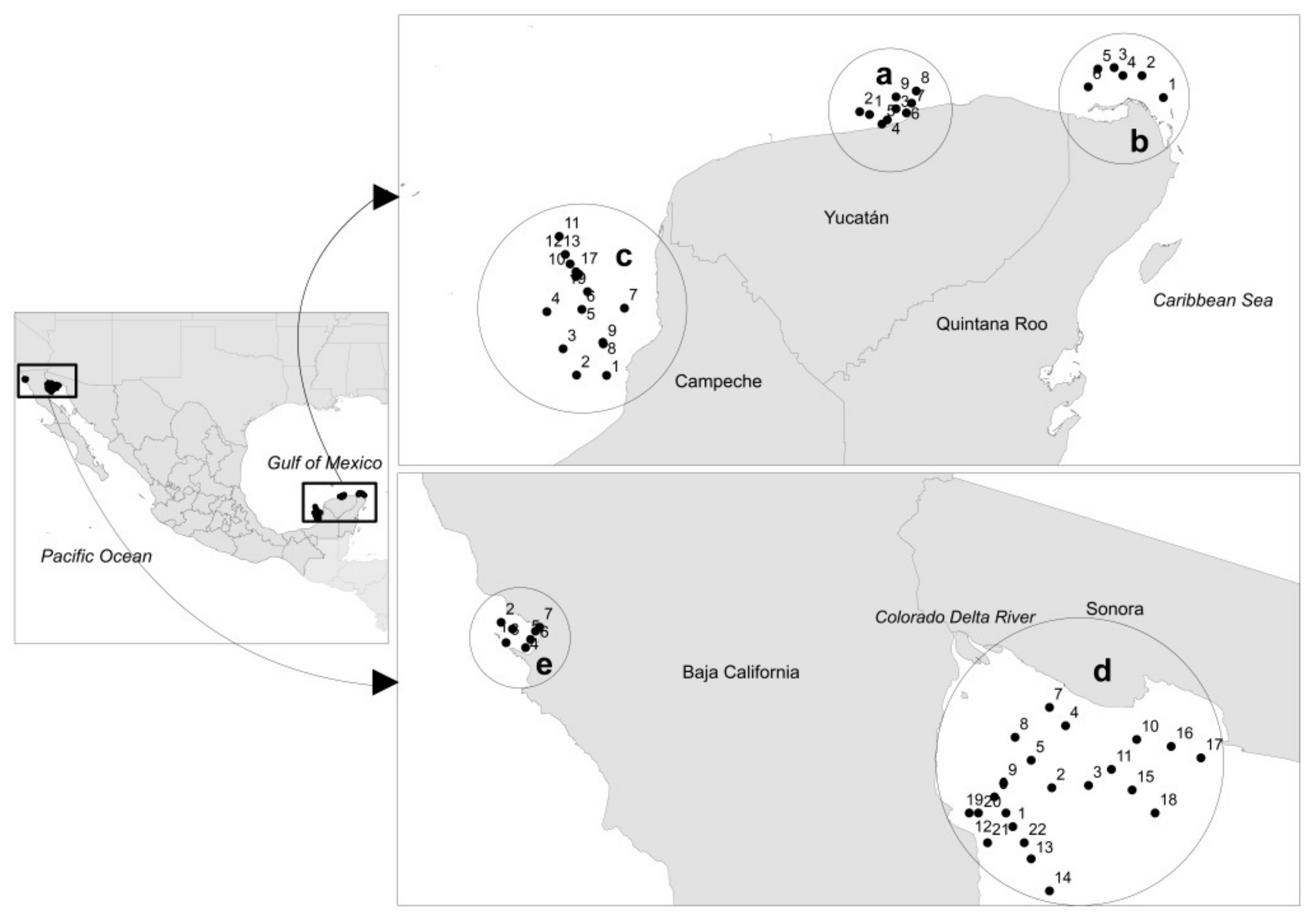
2.1. Study Area

The study areas are well-known coastal areas of Mexico with distinctive characteristics where bloom events have been observed recurrently (Figure 1). These areas are as follows:

Area 1 is composed of three coastal areas in the Yucatán Peninsula: Dzilam de Bravo (Dzilam for short) in the Yucatan state (Figure 1a), Holbox in the Quintana Roo state (Figure 1b), and Campeche Bay in the Campeche state (Figure 1c). This Peninsula is a karstic region, characterized by minimal soil cover and rapid infiltration of rainwater, with the consequent high vulnerability of the aquifer to pollution [25,26]. The rainy season occurs from June through December with minimal rainfall during the rest of the year. According to [27], the Yucatán coastal aquifer is a triple porosity system, where the flow of groundwater takes place mainly through interconnected cave systems and fractures, and drains inland catchments primarily through coastal springs. In recent years, intense coastal development has taken place within the Caribbean, due to tourism, which increases the risk of aquifer pollution. This development is particularly fast on the eastern coast of the Yucatan Peninsula (Quintana Roo state). The unconfined Yucatán aquifer has submarine groundwater discharges (SGDs) threatening coastal ecosystems [26,28]. SGDs have been linked to eutrophication and harmful algal blooms [28]. Both Yucatán and Quintana Roo state coastal waters are influenced by waters of the Caribbean Sea and the Gulf of Mexico [29]. Campeche state coastal water is affected by the current system of Yucatan/Lazo/Florida [30]. This region has a predominantly cyclonic circulation [31], caused by the wind effort [32], and by an upwelling on the north coast of the Yucatan Peninsula [33].

Area 2 is the Upper Gulf of California (UGC). The Gulf of California is a semi-enclosed sea in the Eastern Pacific. The UGC is located in the Northern Gulf of California, where the Sonora and Baja California state coasts intersect at a 60° angle [34]. It is considered as one of the most biologically productive marine regions [35,36], with peak chlorophyll a concentrations of 18.2 mg m⁻³ and averages of 1.8 mg m⁻³ between 1997 and 2007 in coastal waters near the delta [37]. A complex mix of factors increases productivity. Among those are coastal upwelling, wind-driven mixing, extreme tidal mixing and turbulence, thermohaline circulation, coastal-trapped waves, regular sediment resuspension, and, to a lesser extent, agricultural runoff, released nutrients from erosion of ancient Colorado River Delta sediments and groundwater discharges [35,38,39]. After the construction of the Hoover and Glen Canyon dams in the USA in 1935 and 1964, respectively, the Colorado River only discharges variable and insignificant surface water-flows occasionally into the Gulf of California [38].

Area 3, Todos Santos Bay (TSB), is a semi-enclosed bay, adjacent to the Pacific Ocean, within the upwelling zone of the Baja California peninsula (Mexico). This area is influenced by the California Current System (CCS), which produces coastal upwelling along the coast of the Baja California peninsula. A marked seasonality is caused by the prevailing winds from the Northwest, which tend to be more intense during the spring and summer months [40,41,42]. Two water masses integrate the CCS, the California Current (CC), a year-round equatorward surface flow, which transports Subarctic Water (SAW), characterized by low salinity, and the California Undercurrent (CU), a poleward subsurface (100–400 m) flow that transports Equatorial Subsurface Water (ESsW), characterized by relatively high salinity, high nutrient concentration, and low dissolved oxygen content, according to a previous description [43]. The SAW is particularly important during winter and spring, while ESsW appears at the end of summer and autumn [44]. In addition to the described seasonal variability, the El Niño-Southern Oscillation (ENSO) induces oceanographic changes in the region of Baja California at an interannual scale [44]. Together, these factors control primary productivity, which is characteristically high [40,45]. Dinoflagellate algal bloom (DAB) events in this area have increased considerably in extension and frequency over the past two decades [46].

2.2. Collection of Samples

Water samples were collected in Mexico coastal waters at the stations shown in Figure 1. Four field campaigns were conducted for sampling: two in 2011 and two in 2017, during reported bloom events.

Dzilam (Yucatán) and Holbox (Quintana Roo) samples were collected between 27 and 30 of August 2011 (nine and six samples, respectively). All the Dzilam and Holbox stations were sampled at the surface (1.5 m); the selection of monitoring sites was influenced by fishermen reports on fish mortality and patches of discolored water. Campeche Bay (Campeche) samples were collected between 22 and 24 of September 2011 (19 samples). Campeche Bay was also sampled at the surface (1.5 m), except for stations number 13 and 16, which were sampled at 15 m (according to the chlorophyll maximum fluorescence depth). The campaign was conducted in response to a phytoplankton bloom reported by various local, state and federal public health institutions in Campeche [47]. The Todos Santos Bay (TSB) in Ensenada (Baja California) was sampled on 2 June 2017 (seven samples) during the second week of a bloom event that lasted three weeks. This event was characterized by bioluminescence. TSB was also sampled at the surface (0.5 m). Stations 5–7 were located on the reddish patch that distinguished itself from the rest of the bay water.

These data were collected in small vessels where the samples were taken manually and stored in dark Nalgene bottles of high-density polyethylene (HDPE) until processing in the laboratory. For CDOM analysis, samples were collected in amber glass bottles and refrigerated until laboratory processing. The sampling depth was at the chlorophyll maximum fluorescence (0.5 to 15 m). The chlorophyll maximum was measured with a Phyto-PAM (Heinz WalzGmbH, Effeltrich, Germany) fluorimeter.

Sampling of the Upper Gulf of California (UGC) was carried out from 23 February to 3 March 2017, on board the research vessel “Tecolutla” of the Mexican Navy and during the oceanographic cruise “Vaquita Marina 2017” (22 samples). Samples were taken with Niskin bottles attached to a rosette and were immediately processed in the vessel’s laboratory. Sampling depth was at the chlorophyll maximum fluorescence (10 to 40 m). The chlorophyll maximum was measured with an ECO FLNTU fluorimeter coupled to a CTD SB 19 Plus. During the oceanographic cruise, colored patches were detected in the water.

In each study area, the samples were collected inside and outside the patches with bloom evidence to capture the variability that exists in a parcel of water and to better define the baseline or mean of each campaign.

2.3. Absorption Coefficients Determination

Water for CDOM analysis was filtered using a 0.2 μm pore membrane filter (Nuclepore™, Merck KGaA, Darmstadt, Germany) and processed according to the methodology of [48]. The CDOM absorption coefficient, $a_{cdom}\left(\lambda \right)$, was measured in the wavelength range of 250 to 800 nm in a 10 cm long quartz cuvette using Milli-Q water as reference.

The particulate matter absorption coefficient was determined using the methodology of [48]. A volume of seawater of 0.5 to 2 L, depending on the particle load, was filtered from water stored in Nalgene bottles, with Whatman GF/F glass fiber filters 25 mm in diameter and 0.7 μm in pore size. The optical density of particulate material in the filter was measured in the wavelength range of 400 to 800 nm. Then, filters were immersed in methanol to wash out pigments and to obtain the detritus optical density for the same wavelength interval. The light absorption coefficients $a_p\left(\lambda \right)$ and $a_d\left(\lambda \right)$ were calculated following [48], and $a_{phy}\left(\lambda \right)$ was calculated by subtracting $a_d\left(\lambda \right)$ from $a_p\left(\lambda \right)$.

The optical densities of 2011 samples were read with a Perkin-Elmer Lambda 18 (PerkinElmer, Waltham, MA, USA) spectrophotometer, and the 2017 samples were read with a Cary 100 UV-Visible spectrophotometer (Agilent, Santa Clara, CA, USA).

A non-parametric one-way analysis of variance (Kruskal–Wallis) was performed to statistically assess differences in the absorption coefficients. The absorption coefficients $a_{phy}\left(\lambda \right)$, $a_d\left(\lambda \right)$ and $a_{cdom}\left(\lambda \right)$ for each sampling area were compared. Also, sampling stations under active bloom conditions were grouped according to similar phytoplankton absorption coefficients (430–550 nm), as determined by cluster analysis. Clustering dendrograms were generated using Minitab v.16. Correlation distances were calculated, and sampling areas clustered according to the average method.

2.4. IOP Index Determination

The IOP index was determined according to [23] following the next steps. First, the absorption coefficients ($a_{cdom}\left(443\right),a_d\left(443\right),a_{phy}\left(443\right)$) were standardized. Then, principal component analysis (PCA) was performed to reduce the number of original variables. The first principal component was selected because it accounts for the largest possible variance. This selection was based on the eigenvalues [49]. The coefficients of this principal component were named as $b_{1,1},$ $b_{1,2}$ and $b_{1,3}$. Finally, the IOP index was calculated based on this first standardized empirical orthogonal function (SEOF₁) [24] according to Equation (3).

$$IO{P}_{index}=-1\left[(b_{1,1}\times Z{a}_{phy,443})+(b_{1,2}\times Z{a}_{CDOM,443})+(b_{1,3}\times Z{a}_{d,443})\right]$$

(3)

The coefficients $b_{1,1},$ $b_{1,2}$ and $b_{1,3}$ are the first eigenvectors resulting from the SEOF₁, while ($Z{a}_{phy,443},$ $Z{a}_{CDOM,443}$ and $Z{a}_{d,443})$ are the values derived from the Pearson correlation matrix between the absorption coefficients’s standardized anomalies. Then, samples were classified as in bloom or non-bloom using factorial analysis. To describe the stages of a phytoplankton bloom, the values of the IOP index were interpreted as follows [23]: (1) values in the interval (−1, 1) show the average value of the study area and represent non-bloom conditions; (2) values in the interval (1, 2) are above the average and represent decaying bloom conditions, and (3) values higher than 2 are anomalous and indicate active bloom conditions.

2.5. Phytoplankton Community Characterization

The blue/red ratio ($\raisebox{1ex}{$\mathrm{B}$}\!\left/ \!\raisebox{-1ex}{$\mathrm{R}$}\right.$) is an index that allows us to characterize the dominant phytoplankton size in a water sample [24,50,51,52,53,54,55]. It is calculated as expressed in Equation (4):

$$\raisebox{1ex}{$\mathrm{B}$}\!\left/ \!\raisebox{-1ex}{$\mathrm{R}$}\right.=\frac{a_{phy\left(440\right)}}{a_{phy\left(675\right)}}$$

(4)

If the $\raisebox{1ex}{$\mathrm{B}$}\!\left/ \!\raisebox{-1ex}{$\mathrm{R}$}\right.$ is >3.0, dominance of picophytoplankton (<2 μm) is implied. If the ratio is <2.5, dominance of microphytoplankton (>20 μm) is implied. Ratios between 2.5 and 3.0 indicate that the structure of the community in terms of size is dominated by nanophytoplankton.

Representative samples of each sampling event were analyzed by microscopy to identify the main blooming species and/or genus. Samples were preserved in 125 mL bottles in a neutral lugol solution with a sodium acetate base in a 1:100 ratio. The samples were stored under dark and cold conditions until their identification. The Dzilam, Holbox, and Campeche samples were identified by the Florida Fish and Wildlife Conservation Commission (FWC). Phytoplankton identification was performed using an inverted Olympus IX71 microscope following a modified method of Utermöhl [56]. In the case of the UGC and TSB samples, the same method was performed using phase contrast microscopy with a Bausch and Lomb microscope. The authors [57,58,59,60] were used as taxonomic references.

For Dzilam, Holbox and Campeche, the chlorophyll a concentration was determined fluorometrically on methanol extracts following the method of [61], using a Turner Designs 10-AU field fluorimeter.

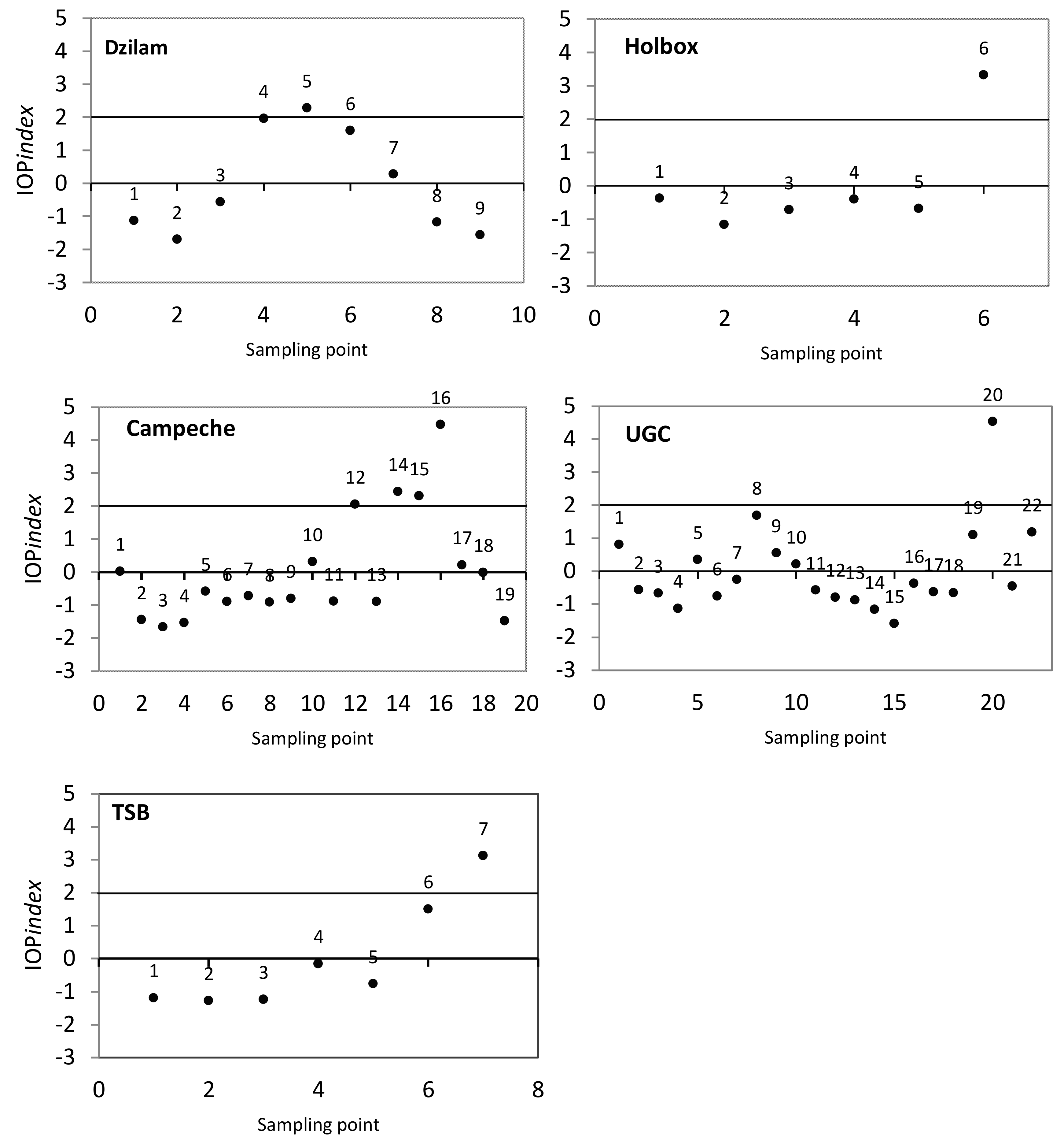
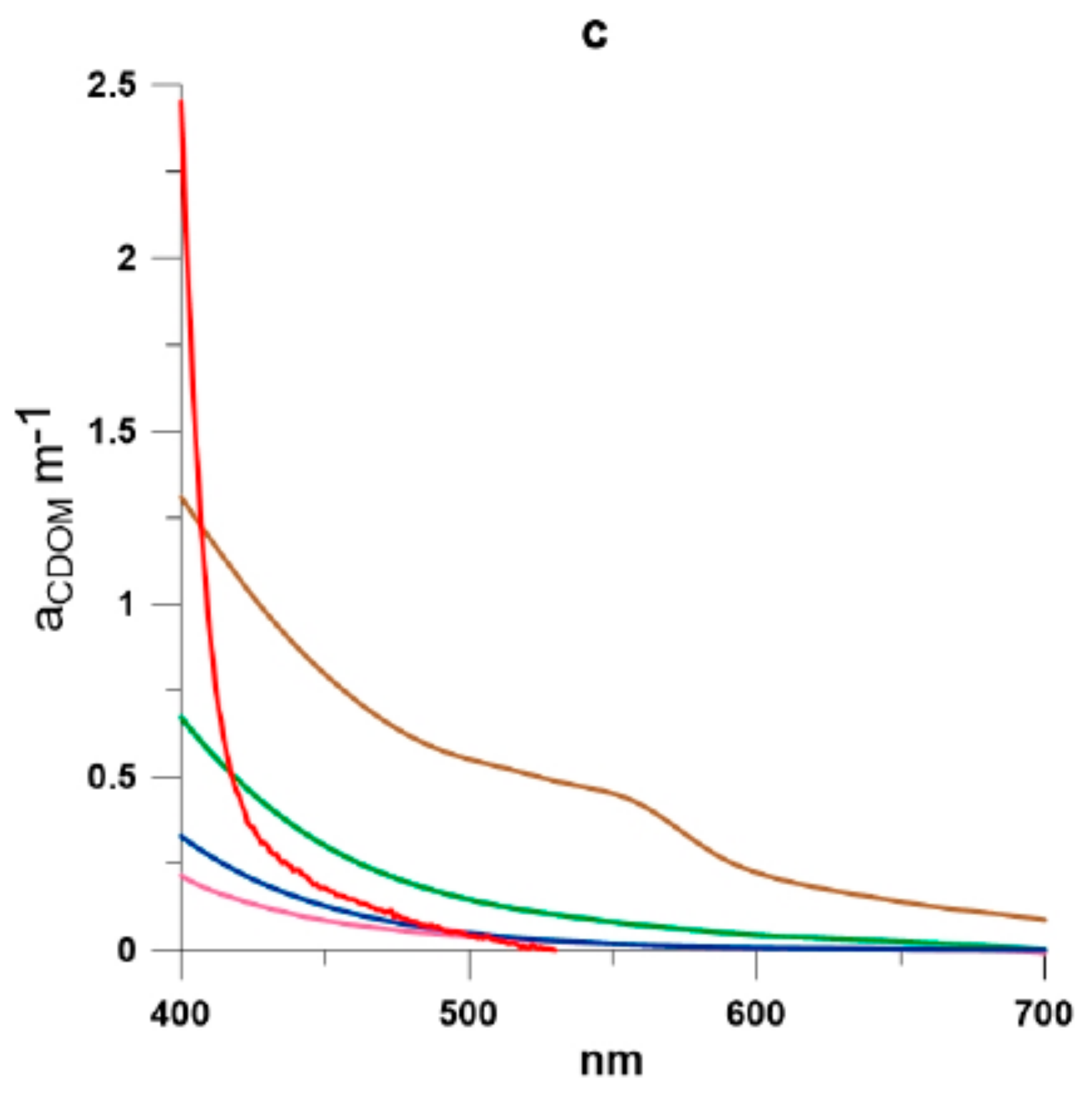
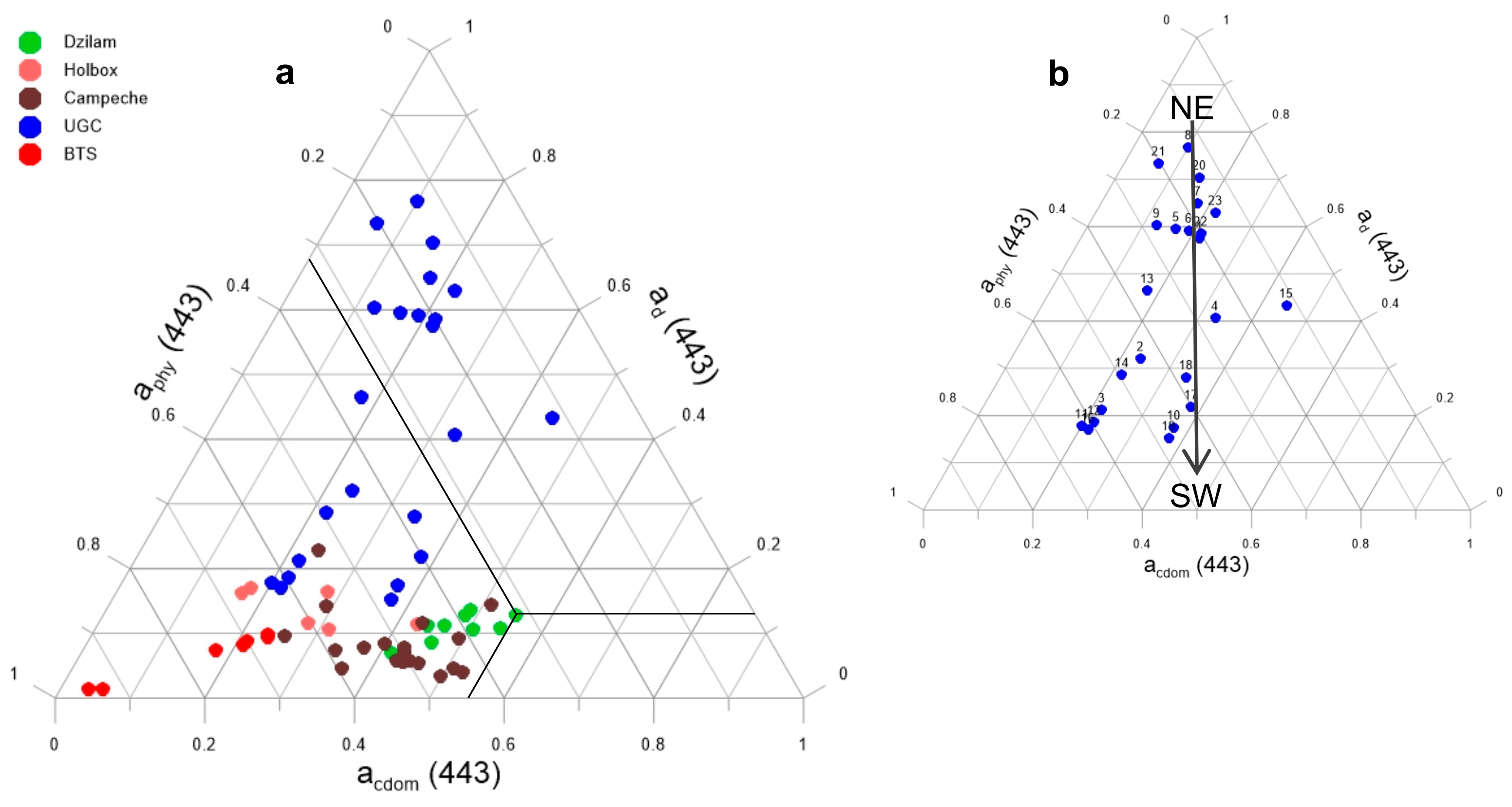
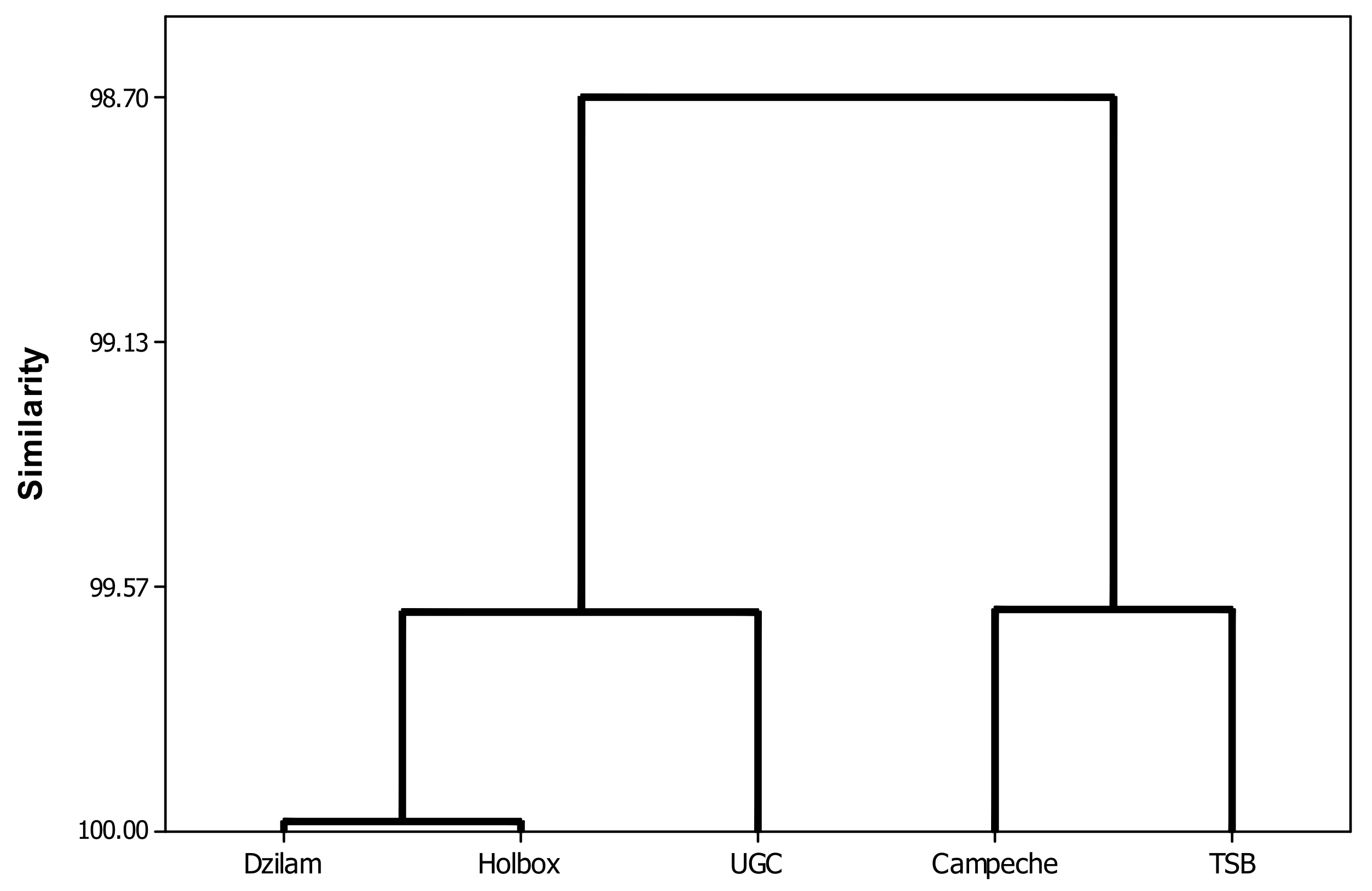
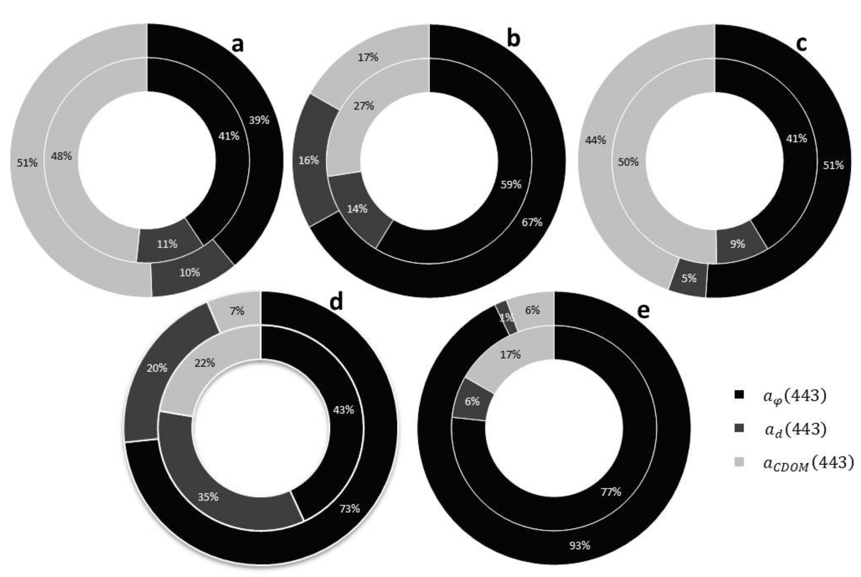
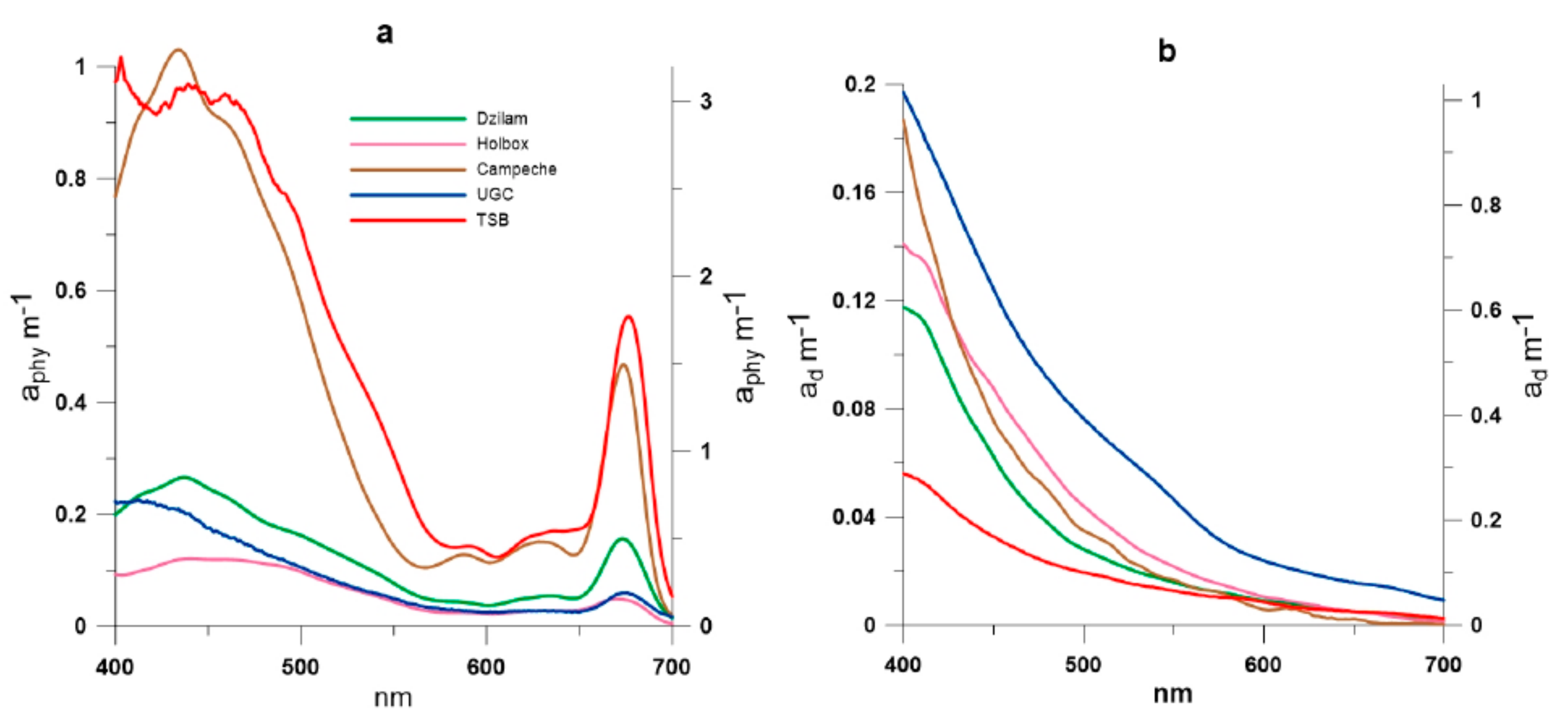
3. Results and Discussion

The IOP index was calculated from the absorption coefficients for each sampling area and sampling point. IOP index results are represented graphically in Figure 2. In Dzilam, sampling points 4 and 6 had a value in the interval (1, 2), meaning that they were above the sampling area average and in decaying bloom conditions. However, only sampling point 5 was above two and under active bloom conditions. In Figure 3, the contribution of each absorption coefficient ($a_{phy}\left(443\right),$ $a_d\left(443\right)$ and $a_{cdom}\left(443\right)$) to $a\left(443\right)$ by sampling area is represented. The inner circumference shows the average contribution of each absorption coefficient to $a\left(443\right)$ for each sampling campaign. The outer circumference represents the average value of sampling points classified as active bloom according to the IOP index. In Figure 3a, Dzilam, CDOM was the major contributor to $a\left(443\right)$. $a_{cdom}\left(443\right)$ contributed with 48% to total absorption, followed by $a_{phy}\left(443\right)$ with 41% and $a_d\left(443\right)$ with 11% (Figure 3a). At sampling point 5, we observed that the contribution of each absorption coefficient to $a\left(443\right)$ was similar to the sampling campaign average. In Holbox, only sampling point 6 was above an IOP index value of two (Figure 2), and thus under active bloom conditions. Phytoplankton was the major contributor to $a\left(443\right)$. $a_{phy}\left(443\right),$ representing 59% of absorption, followed by $a_{cdom}\left(443\right)$ with 27% and $a_d\left(443\right)$ with 14% (Figure 3b). At sampling point 6, we observed a higher contribution of phytoplankton to $a\left(443\right)$ than the average value of the sampling campaign ($a_{phy}\left(443\right)$ of 67%). The lower average contribution of phytoplankton when considering all sampling points was related to a higher CDOM contribution under non-bloom conditions. In Campeche Bay, sampling points 12, 14, 15 and 16 were under active bloom conditions (Figure 2). Sampling point 16 showed the highest anomaly; this sample was collected at 15 m depth. In Figure 3c, the dominant absorption component was $a_{cdom}\left(443\right)$ with 50%, as in Dzilam, followed by $a_{phy}\left(443\right)$ with 41% of $a\left(443\right)$, and a minor contribution of $a_d\left(443\right)$ (9%). At sampling point 16 (the one that is represented in the outer circumference, Figure 3c), we observed a higher contribution of phytoplankton. This was due to a higher CDOM contribution under non-bloom conditions. In the Upper Gulf of California (UGC), sampling points 8, 19 and 22 were in decaying bloom conditions (IOP index value higher than one and lower than two), while sampling station 20 was under active bloom conditions according to the IOP index (Figure 2). In Figure 3d, we observed that the highest contribution was from $a_{phy}\left(443\right),$ with 43%, followed by $a_d\left(443\right)$ with 35% of $a\left(443\right)$, and $a_{cdom}\left(443\right)$ with 22% (Figure 3d). As in Holbox and Campeche Bay, the contribution of phytoplankton to $a\left(443\right)$ was higher than the average in the active bloom stations ($a_{phy}\left(443\right)$ of 73% for sampling point 20). In Todos Santos Bay, sampling point 6 was under decaying bloom conditions, while sampling point 7 was under active bloom conditions. In Todos Santos Bay (TSB) (Figure 3e), as in Holbox, $a_{phy}\left(443\right)$ represented the highest absorption percentage (77%). However, in TSB the contribution of $a_{cdom}\left(443\right)$ and $a_d\left(443\right)$ was characteristically low (17% and 6%, respectively). As in Holbox, Campeche Bay and UGC, we noticed a higher contribution of phytoplankton to $a\left(443\right)$ in the active bloom station ($a_{phy}\left(443\right)$ of 93% for sampling point 7).$\mathrm{The} a_{cdom}\left(443\right)$ and $a_d\left(443\right)$ contribution was even lower than the average.

In Figure 4, the absorption spectrum of phytoplankton, detritus and CDOM of all the stations in bloom is compared. In the case of Campeche, the station in bloom with the greatest anomaly is represented. The phytoplankton absorption coefficient, $a_{phy}\left(\lambda \right)$, was significantly higher in TSB than in other sampling areas (p < 0.05 for $a_{phy}$(443)). No significant differences were observed between Dzilam and Campeche Bay (p > 0.05 for $a_{phy}$(443). The lowest $a_{phy}\left(\lambda \right)$ values were observed in the UGC. The detritus absorption coefficient, $a_d\left(\lambda \right)$, was significantly higher in the UGC than in all the other studied areas (p < 0.05 for $a_d\left(443\right)$). No significant differences were observed between the Yucatan Peninsula areas (Dzilam, Holbox and Campeche) or with TSB (p > 0.05 for $a_d\left(443\right)$). The CDOM absorption coefficient, $a_{cdom}\left(\lambda \right)$, was significantly higher in Dzilam and Campeche Bay than in other areas (p < 0.05 for $a_d\left(443\right)$).

In Figure 5, the ternary diagram shows the contribution to absorption of each seawater component (phytoplankton, detritus and colored dissolved organic matter) for all the sampling points. This graphical representation allowed us to compare the different study areas. In general terms, most areas have a stronger contribution from phytoplankton $(a_{phy}\left(443\right))$ and CDOM ($a_{cdom}\left(443\right))$ with the exception of UGC where some stations had a stronger contribution from detritus (a_d(443)). However, this high detritus contribution was much more important near the Colorado River Delta and decreased southward (Figure 5a).

In order to characterize the phytoplankton community, the blue/red ratio ($\raisebox{1ex}{$\mathrm{B}$}\!\left/ \!\raisebox{-1ex}{$\mathrm{R}$}\right.$) is shown in

Table 1. Specific absorption coefficients of phytoplankton (a_phy) at 440 nm and 675 nm (m⁻¹), and blue/red ratio (B/R) (a_phy(440)/a_phy(675)) based on the samples collected in the five campaigns.

Campaign	Sta.	aphy (440 nm)	aphy (675 nm)	Ratio B/R	Campaign	Sta.	aphy (440 nm)	aphy (675 nm)	Ratio B/R
Dzilam	1	0.110	0.038	2.86	UGC	1	0.039	0.078	1.99
	2	0.091	0.032	2.83		2	0.035	0.084	2.40
	3	0.167	0.061	2.75		3	0.039	0.095	2.43
	4	0.371	0.229	1.62		4	0.017	0.042	2.47
	5	0.264	0.155	1.71		5	0.041	0.085	2.07
	6	0.179	0.064	2.80		6	0.024	0.054	2.27
	7	0.170	0.072	2.36		7	0.026	0.055	2.09
	8	0.131	0.035	3.79		8	0.036	0.084	2.35
	9	0.131	0.028	4.76		9	0.048	0.105	2.16
Holbox	1	0.101	0.030	3.36		10	0.038	0.093	2.43
	2	0.076	0.023	3.37		11	0.045	0.105	2.31
	3	0.118	0.038	3.08		12	0.043	0.093	2.18
	4	0.072	0.024	3.06		13	0.031	0.073	2.33
	5	0.094	0.028	3.34		14	0.032	0.073	2.28
	6	0.387	0.151	2.57		15	0.003	0.007	2.59
Campeche	1	0.067	0.016	4.28		16	0.029	0.066	2.24
	2	0.034	0.006	5.33		17	0.032	0.071	2.21
	3	0.036	0.006	6.47		18	0.028	0.066	2.35
	4	0.032	0.006	5.24		19	0.032	0.073	2.27
	5	0.136	0.054	2.53		20	0.020	0.072	3.54
	6	0.111	0.044	2.51		21	0.059	0.201	3.39
	7	0.129	0.027	4.80		22	0.021	0.053	2.57
	8	0.132	0.028	4.77		23	0.026	0.067	2.55
	9	0.114	0.030	3.83	TSB	1	0.144	0.053	2.70
	10	0.295	0.154	1.91		2	0.139	0.047	2.96
	11	0.135	0.067	2.02		3	0.172	0.061	2.82
	12	0.685	0.338	2.03		4	0.365	0.150	2.43
	13	0.127	0.052	2.43		5	0.219	0.085	2.58
	14	0.590	0.287	2.06		6	3.077	1.773	1.74
	15	0.543	0.251	2.17		7	3.617	1.815	1.99
	16	1.006	0.464	2.17
	17	0.370	0.172	2.16
	18	0.243	0.114	2.13
	19	0.065	0.021	3.09

. As previously mentioned $\raisebox{1ex}{$\mathrm{B}$}\!\left/ \!\raisebox{-1ex}{$\mathrm{R}$}\right.$ values higher than 3 reveal a community dominated by picophytoplankton; $\raisebox{1ex}{$\mathrm{B}$}\!\left/ \!\raisebox{-1ex}{$\mathrm{R}$}\right.$ values lower than 2.5 reveal microphytoplankton dominance; and $\raisebox{1ex}{$\mathrm{B}$}\!\left/ \!\raisebox{-1ex}{$\mathrm{R}$}\right.$ values between 2.5 and 3.0 indicate that the size structure is dominated by pico/nano-phytoplankton.

In Dzilam, microphytoplankton dominated in the active bloom sampling point 5, where phytoplankton abundance exceeded 1 million cells L⁻¹ ($\raisebox{1ex}{$\mathrm{B}$}\!\left/ \!\raisebox{-1ex}{$\mathrm{R}$}\right.$ = 1.71) (Table 1). According to the microscope taxonomic analysis, the dominant species was the diatom Rhizosolenia hebetata.

In Holbox, the $\raisebox{1ex}{$\mathrm{B}$}\!\left/ \!\raisebox{-1ex}{$\mathrm{R}$}\right.$ ratio under active bloom sample 6 was 2.57 (Table 1), which indicated a mixed picophytoplanton and nanophytoplankton community, where phytoplankton abundance almost reached 1.5 million cells L⁻¹. This was corroborated by microscope taxonomic analysis that identified the dinoflagellate Scrippsiella sp., and the diatoms Chaetoceros sp. and Rhizosolenia hebetata.

In Campeche Bay, $\raisebox{1ex}{$\mathrm{B}$}\!\left/ \!\raisebox{-1ex}{$\mathrm{R}$}\right.$ was lower than 2.5 in all active bloom condition points (Table 1), so microphytoplankton was dominant, and phytoplankton abundance exceeded 1 million cells L⁻¹. The dinoflagellate Karenia brevis was identified by microscopy as the dominant species.

In the UGC, $\raisebox{1ex}{$\mathrm{B}$}\!\left/ \!\raisebox{-1ex}{$\mathrm{R}$}\right.$ was below 2.5 in nearly all the sampling stations (Table 1). However, in sampling 15, $\raisebox{1ex}{$\mathrm{B}$}\!\left/ \!\raisebox{-1ex}{$\mathrm{R}$}\right.$ was 2.59, indicating a community dominated by the pico/nano-phytoplankton, where phytoplankton abundance just exceeded 4 thousand cells L⁻¹. The diatoms Coscinodiscus sp. and Pseudo-nitzschia sp. were identified by microscopy.

In Todos Santos Bay, $\raisebox{1ex}{$\mathrm{B}$}\!\left/ \!\raisebox{-1ex}{$\mathrm{R}$}\right.$ was below 2.5 at sampling point 7 (active bloom conditions) (Table 1), thus indicating microphytoplankton dominance, where phytoplankton abundance exceeded 40 thousand cells L⁻¹. The most abundant species in this station was the dinoflagellate Lingulodinium polyedrum.

In Figure 6, sampling stations under active bloom conditions are grouped according to similar phytoplankton absorption coefficients (wavelength ranging from 430 to 550 nm). The dendogram is the result of the cluster analysis. Sampling stations are named according to the study area that they represent. Dzilam, Holbox and UGC are grouped into one cluster; these sampling stations are characterized by high diatom abundance. Dzilam and Holbox share the same species (Rhizosolenia hebetata). Campeche and TSB are grouped into another cluster; these stations are characterized by dinoflagellates species. Thus, stations with similar species composition exhibit similar absorption spectra.

Dzilam (Yucatan), Holbox (Quintana Roo), and Campeche Bay (Campeche) (Figure 1a–c) are located in the karstic Yucatan Peninsula [55]. Rapid rainwater infiltration into the groundwater system and nearly no surface runoff characterize this region [25,29]. Due to its hydrological characteristics, the lowest absorption coefficient is that of detritus ($a_d\left(443\right)$ is 11%, 14% and 9%, respectively, in each area) (Figure 4). There is no relevant detritus source and no river runoff in this area (the nearest one is located in southern Campeche, far from the sampling area located in north Campeche). The climate of the region is characterized by three seasons associated with rainfall patterns: the dry season (March to May), the rainy season (June to October) and the northern wind season [62]. In this region, submarine groundwater discharges (SGDs) play a significant role in driving the nutrient stoichiometry (N:Si:P ratio) in receiving waters, which is a key factor for phytoplankton assemblages. SGDs are an important source of nitrogen, particularly ${\mathrm{NO}}_3^{-}$; during the wet season (June to October), the high N:P ratio in SGDs can drive phosphorus limitation in the nearshore environment [27]. SGDs are also rich in silica, which can lead to diatom growth. Several studies have concurred that low salinity groundwater is an important source of nutrients in the Yucatan, specifically ${\mathrm{NO}}_3^{-}$ and silica, and have linked SGDs to harmful algal blooms [27]. According to [63], the HAB events in the state of Yucatan have been reported almost every year since 2001, covering an approximate area of 6000 km².

Our sampling was developed during the large-scale pelagic bloom event of August–December 2011. This event started in Dzilam and tended to move westward along the northern Yucatan coast [64]. In Dzilam, the dominance of the diatom Rhizosolenia hebetata can be explained by the input of silica from nearby springs (cenotes). The authors of [64] observed maximum chlorophyll a concentrations on 8 and 30 August. Our sampling was performed on 27 August. Therefore, the degradation of phytoplankton cells from the previous peak may explain the high contribution of the CDOM absorption coefficient (48% on average). The sampling point identified as being under active bloom conditions according to the IOP index had significantly higher chlorophyll a levels, 12.5 mg m⁻³, which indicates non-bloom conditions, i.e., 3.1 mg m⁻³ on average.

In Holbox, the diatoms Chaetoceros sp. and Rhizosolenia hebetata were also dominant, but dinoflagellates of Scrippsiella sp. were also abundant. Both Chaetoceros sp. and Scrippsiella sp. were also observed in Dzilam during this HAB event according to [64]. The silica needed for this sustained diatom bloom may have been supplied by the characteristic springs (cenotes) of the Quintana Roo state [65]. The sample identified as under active bloom conditions according to the IOP index had significantly higher chlorophyll a levels (12.5 mg m⁻³) than samples in non-bloom conditions (around 2.2 mg m⁻³ on average).

In Campeche Bay, the blooming species was identified as the dinoflagellate Karenia brevis. Karenia brevis blooms have been observed in all Mexican states (except Quintana Roo) [65]. Again, in this sampling campaign, the sampling point under active bloom conditions according to the IOP index had significantly higher chlorophyll a levels (33.2 mg m⁻³) than sampling points in non-bloom conditions (7.0 mg m⁻³ on average). The CDOM absorption coefficient, $a_{cdom}\left(443\right)$, was as high as in Dzilam (higher than in all the other study areas) (Figure 3). Our sampling was performed on 22 September 2011. Therefore, the high CDOM values could be explained by the degradation of accumulated phytoplankton cells during August and September. This region is influenced by the current system of Yucatan/Lazo/Florida [30]. It is important to note that even under very high CDOM values, the IOP index was able to distinguish an active phytoplankton bloom.

The Upper Gulf of California (UGC) and Colorado River Delta (CRD) area is a region of sediment re-suspension characterized by high detritus levels, low light extinction coefficient values (−0.05 m⁻¹) and high sedimentary loads (maximum values of 8 g/L) [34,39]. Therefore, we expected the highest detritus absorption coefficient ($a_d\left(\lambda \right)$) to be observed. It is remarkable that, also under very high detritus levels, the IOP index was able to distinguish an active phytoplankton bloom. Both genera found in the UGC, Coscinodiscus sp. and Pseudo-nitzschia sp., are indicators of marine conditions rich in nutrients or upwelling [66,67,68]. Pseudo-nitzschia abundances from 1 to 34 × 10³ cells L⁻¹ have been considered as in bloom conditions [69].

In Todos Santos Bay (TSB), the most abundant species during our study was the dinoflagellate Lingulodinium polyedrum. The authors of [46] have reported an increase in dinoflagellate algal blooms (DABs), with Lingulodinium polyedrum as the dominant species, over the past few years in coastal areas off Baja California. Our sampling took place on 2 June 2017, which is late spring, when L. polyedrum blooms usually occur in this area [46]. These blooms have been related to increases in irradiance, daylight hours, temperatures between 17 and 23 °C, stratification of the water column and formation of a seasonal surface thermocline [70]. They are favoured by the convergence of surface currents and winds, which induce the transport of cells that tend to concentrate near the surface and toward the coast [45,71]. The highest phytoplankton absorption coefficient ($a_{phy}\left(\lambda \right)$) throughout the study was assigned to this bloom (Figure 4).

HAB’s are often divided into toxic versus high-biomass blooms [72]. The genus observed in the UGC was Pseudo-nitzschia, a diatom which produces Amnesic Shellfish Poisoning and Domoic Acid Poisoning; despite that the cell concentration was too low to produce a toxic effect (approximately 1000 cell L⁻¹), it was classified as a high-biomass bloom by the IOP index. Blooms of dinoflagellates such as Lingulodinium are yessotoxin producers [72]. In our study area, this genus was observed in TSB with higher frequency, but they have been reported in California and along the West Coast of the US as an emerging potential threat [72].

Research-based forecast systems for toxic blooms are the preoccupation of HAB monitoring networks. The list of predictor variables includes chlorophyll a, macronutrients, and upwelling. Based on our results, we think that absorption coefficients must also be included in this list. Using the IOP index could reduce the cost of regulatory analysis, as it could help in determining which samples should be analyzed with more costly analytical methods, before beach closure or other management decisions. In this sense, the capability of the IOP index is crucial to distinguish between active or decaying bloom. Fixing techniques do not allow this distinction by microscopic counts and thus can lead to worse decisions. The development of common methodologies and approaches in international networks affected by transboundary problems is important. For instance, the California Harmful Algal Bloom Monitoring and Alert Program, or CalHABMAP, integrates groups across the US region but contemplates expansion to include both Mexican observations and observations from the other western states [72].

4. Conclusions

The selected study areas have allowed us to apply the IOP index within the wide variability of optically complex coastal waters. Within this variability, we found areas with dominance of detritus or CDOM, despite the samplings being developed in areas with observed phytoplankton blooms. The IOP index was able to discern sampling points under active bloom conditions from points in decaying bloom conditions. In the Yucatan region, the IOP index distinguished points under active bloom from points with high CDOM due to phytoplankton cell degradation from previous blooms. Also, the IOP index has been proved useful to distinguish phytoplankton blooms from the natural variability of an area. In the case of the UGC, typical high detritus levels produce a high absorption coefficient, which is not related to phytoplankton blooms. The IOP index was able to identify points under active bloom conditions from points with a high detritus load.

Continuous monitoring is essential to be able to distinguish a phytoplankton bloom from natural variability. The inherent optical properties play a key role in correctly identifying phytoplankton blooms, but are highly variable in complex coastal waters. Baseline values are unique to a coastal area and should be defined to enable the detection of anomalous events. Thus, the measurement of absorption coefficients should be considered in programs monitoring coastal waters.

In this research, the IOP index has been applied in optically complex coastal waters. However, it could also be applied to inland waters because they share the same bio-optical principle of absorption and refraction of light by particles contained in water. In inland waters, the optically active substances can vary in type and quantity in short time intervals and are often more noticeable than those occurring in the ocean [73]. Therefore, the IOP index could also be used in inland water monitoring programs, such as in the EU Water Framework Directive (Directive 2000/60/EC).

The importance of defining the baseline for the interpretation of the IOP index should be underlined. The definition of the average values of a specific area allows identifying the sampling points that have anomalous values. For this reason, it is important to have a wide range of data during the sampling, but also an adequate distribution that allows us to evaluate the variability of the studied area and to better define the baseline. The use of remote sensing can help to define IOPs from satellite reflectances, $R_{rs}\left(\lambda \right)$, and to build a baseline at a lower cost. In-situ IOP measurements could be compared to this baseline to identify active phytoplankton blooms using the IOP index. Further research is needed to test the benefits and limits of this methodology.

References

1. Gower, J.; King, S.; Borstad, G.; Brown, L. Detection of intense plankton blooms using the 709 nm band of the MERIS imaging spectrometer. Int. J. Remote Sens. 2005, 26, 2005–2012. [Google Scholar] [CrossRef]
2. Carstensen, J.; Conley, D. Frequency, composition, and causes of summer phytoplankton blooms in a shallow coastal ecosystem, the Kattegat. Limnol. Oceanogr. 2004, 49, 191–201. [Google Scholar] [CrossRef]
3. Legendre, L. The significance of microalgal blooms for fisheries and for the export of particulate organic carbón in oceans. J. Plankton Res. 1990, 12, 681–699. [Google Scholar] [CrossRef]
4. Ji, R.; Edwards, M.; Mackas, D.; Runge, J.; Thomas, A. Marine plankton phenology and life history in a changing climate: Current research and future directions. J. Plankton Res. 2010, 32, 1355–1368. [Google Scholar] [CrossRef] [PubMed]
5. Richardson, K. Harmful or exceptional phytoplankton blooms in the marine ecosystem. Adv. Mar. Biol. 1997, 31, 301–385. [Google Scholar] [CrossRef]
6. Smayda, T.J. What is a bloom? A commentary. Limnol. Oceanogr. 1997, 42, 1132–1136. [Google Scholar] [CrossRef]
7. Brody, S.R.; Lozier, M.S.; Dunne, J.P. A comparison of methods to determine phytoplankton Bloom initiation. J. Geophys. Res. Oceans 2013, 118, 2345–2357. [Google Scholar] [CrossRef]
8. Platt, T.; Fuentes-Yaco, C.; Frank, K.T. Spring algal Bloom and larval fish survival. Nature 2007, 423, 398–399. [Google Scholar] [CrossRef] [PubMed]
9. Schneider, B.; Kaitala, S.; Maunula, P. Identification and quantification of plankton bloom events in the Baltic Sea by continuous pCO2 and chlorophyll a measurements on a cargo ship. J. Mar. Syst. 2006, 59, 238–248. [Google Scholar] [CrossRef]
10. Gittings, J.A.; Raitsos, D.E.; Racault, M.F.; Brewin, R.J.; Pradhan, Y.; Sathyendranath, S.; Platt, T. Seasonal phytoplankton blooms in the Gulf of Aden revealed by remote sensing. Remote Sens. Environ. 2017, 189, 56–66. [Google Scholar] [CrossRef]
11. Huppert, A.; Blasius, B.; Stone, L. A Model of Phytoplankton Blooms. Am. Nat. 2002, 159, 156–171. [Google Scholar] [CrossRef] [PubMed]
12. Fleming, V.; Seppo Kaitala, S. Phytoplankton spring bloom intensity index for the Baltic Sea estimated for the years 1992 to 2004. Hydrobiologia 2006, 554, 57–65. [Google Scholar] [CrossRef]
13. Carstensen, J.; Henriksen, P.; Heiskanen, A.-S. Summer algal blooms in shallow estuaries: Definition, mechanisms, and link to eutrophication. Limnol. Oceanogr. 2007, 52, 370–384. [Google Scholar] [CrossRef]
14. Cetinic, I.; Perry, M.J.; D’Asaro, E.; Briggs, N.; Poulton, N.; Sieracki, M.E.; Lee, C.M. A simple optical index shows spatial and temporal heterogeneity in phytoplankton community composition during the 2008 North Atlantic Bloom Experiment. Biogeosciences 2015, 12, 2179–2194. [Google Scholar] [CrossRef]
15. Alikas, K.; Kangro, K.; Reinart, A. Detecting cyanobacterial blooms in large North European lakes using the Maximum Chlorophyll Index. Oceanologia 2010, 52, 237–257. [Google Scholar] [CrossRef]
16. Platt, T.; Sathyendranath, S.; White, G.; Fuentes-Yaco, C.; Zhai, L.; Devred, E.; Tang, C. Diagnostic properties of phytoplankton time series from remote sensing. Estuar. Coasts 2009, 33, 428–439. [Google Scholar] [CrossRef]
17. Preisendorfer, R.W. Application of Radiative Transfer Theory to Light Measurements in the Sea; IUGG: Potsdam, Germany, 1961; Volume 10, pp. 11–30. [Google Scholar]
18. Cui, T.; Cao, W.; Zhang, J.; Hao, Y.; Yu, Y.; Zu, T.; Wang, D. Diurnal variability of ocean optical properties during a coastal algal bloom: Implications for ocean colour remote sensing. Int. J. Remote Sens. 2013, 34, 8301–8318. [Google Scholar] [CrossRef]
19. Loisel, H.; Vantrepotte, V.; Norkvist, K.; Mériaux, X.; Kheireddine, M.; Ras, J.; Pujo-Pay, M.; Combet, Y.; Leblanc, K.; Dall’Olmo, G.; et al. Characterization of the Bio-Optical Anomaly and Diurnal Variability of Particulate Matter, as Seen from Scattering and Backscattering Coefficients, in Ultra-Oligotrophic Eddies of the Mediterranean Sea. Biogeosciences 2011, 8, 3295–3317. [Google Scholar] [CrossRef]
20. Mercado, J.M.; Ramírez, T.; Cortés, D.; Sebastián, M.; Reul, A.; Bautista, B. Diurnal Changes in the Bio-Optical Properties of the Phytoplankton in the Alborán Sea (Mediterranean Sea). Estuar. Coast. Shelf Sci. 2006, 69, 459–470. [Google Scholar] [CrossRef]
21. Kirk, J.T.O. Light and Photosynthesis in Aquatic Ecosystems, 3rd ed.; Cambridge University Press: Cambridge, UK, 2011; ISBN 9780521151757. [Google Scholar]
22. Morel, A. Meeting the Challenge of Monitoring Chlorophyll in the Ocean from Outer Space. In Chlorophylls and Bacteriochlorophylls: Biochemistry, Biophysics, Functions and Applications; Grimm, B., Porra, R., Rüdiger, W., Scheer, H., Eds.; Springer: Dordrecht, The Netherlands, 2006; Volume 25, pp. 521–534. ISBN 978-1-4020-4516-5. [Google Scholar]
23. Santamaría-del-Angel, E.; Soto, I.; Millán-Nuñez, R.; González-Silvera, A.; Wolny, J.; Cerdeira-Estrada, S.; Cajal-Medrano, R.; Muller-Karger, F.; Cannizzaro, J.; Padilla-Rosas, Y.; et al. Experiences and Recommendations for Environmental Monitoring Programs. In Environmental Science, Engineering and Technology; Sebastia-Frasquet, M.-T., Ed.; Nova Science Publishers: Hauppauge, NY, USA, 2015; p. 32. ISBN 978-1-63482-189-6. [Google Scholar]
24. Santamaría-del-Angel, E.; González-Silvera, A.; Millán-Nuñez, R.; Callejas-Jiménez, M.E.; Cajal-Medrano, R. Determining Dynamic Biogeographic Regions using Remote Sensing Data. In Handbook of Satellite Remote Sensing Image Interpretation: Applications for Marine Living Resources Conservation and Management; Morales, J., Stuart, V., Platt, T., Sathyendranath, S., Eds.; EU PRESPO and IOCCG: Dartmouth, NS, Canada, 2011; Chapter 19; pp. 273–293. [Google Scholar]
25. Hernández-Terrones, L.; Rebolledo-Vieyra, M.; Merrino-Ibarra, M.; Soto, M.; LeCossee, A.; Monroy-Rios, E. Groundwater pollution in karstic region (NE Yucatán): Baseline nutrient content and flux to coastal ecosystems. Water Air Soil Pollut. 2011, 218, 517–528. [Google Scholar] [CrossRef]
26. Moore, Y.H.; Stoessell, R.K.; Easley, D.H. Fresh-Water/Sea-Water Relationship within a Ground-Water Flow System, Northeastern Coast of the Yucatan Peninsula. Groundwater 1992, 30, 343–350. [Google Scholar] [CrossRef]
27. Beddows, P.A.; Smart, P.L.; Whitaker, F.F.; Smith, S.L. Decoupled fresh-saline groundwater circulation of a coastal carbonate aquifer: Spatial patterns of temperature and specific electrical conductivity. J. Hydrol. 2007, 346, 18–32. [Google Scholar] [CrossRef]
28. Hernández-Terrones, L.M.; Null, K.A.; Ortega-Camacho, D.; Paytan, A. Water quality assessment in the Mexican Caribbean: Impacts on the coastal ecosystem. Cont. Shelf Res. 2015, 102, 62–72. [Google Scholar] [CrossRef]
29. Herrera-Silveira, J.A.; Morales-Ojeda, S.M. Subtropical Karstic Coastal Lagoon Assessment, Southeast Mexico. The Yucatan Peninsula Case. In Coastal Lagoons: Critical Habitats of Environmental Change; Kennish, M.J., Paerl, H.W., Eds.; CRC Press: Boca Raton, FL, USA, 2010; p. 26. ISBN 9781420088304 1420088300. [Google Scholar]
30. Sánchez, F.J.; Gámez, D.; Guevara, G.; Shirasago, G.; Obeso, M. Análisis de la circulación superficial de mesoescala en la bahía de Campeche mediante sensores activos y pasivos. Geos 2010, 30, 204. [Google Scholar]
31. Monreal-Gómez, M.A.; Salas de León, D.A. Simulación de la circulación en la Bahía de Campeche. Geofís. Int. 1990, 29, 101–111. [Google Scholar]
32. Merrell, W., Jr.; Morrison, J. On the circulation of the western Gulf of Mexico with observations from April 1978. J. Geophys. Res. 1981, 86, 4181–4185. [Google Scholar] [CrossRef]
33. Cochrane, J.D. Investigations of the Yucatan current; the region of cold surface water. In Oceanography and Meteorology of the Gulf of Mexico; McLellan, H.J., Ed.; Annual Report Rep 61-15F; Department of Oceanography, Texas A&M University: College Station, TX, USA, 1961; pp. 5–6. [Google Scholar]
34. Carriquiry, J.D.; Sanchez, A. Sedimentation in the Colorado River delta and Upper Gulf of California after nearly a century of discharge loss. Mar. Geol. 1999, 158, 125–145. [Google Scholar] [CrossRef]
35. Brusca, R.C.; Álvarez-Borrego, S.; Hastings, P.A.; Findley, L.T. Colorado River flow and biological productivity in the Northern Gulf of California, Mexico. Earth Sci. Rev. 2017, 164, 1–30. [Google Scholar] [CrossRef]
36. Santamaría-del Ángel, E.; Millán-Núñez, R.; De la Peña, G. Efecto de la turbidez en la productividad primaria en dos estaciones en el Área del Delta del Río Colorado. Cienc. Mar. 1996, 22, 483–493. [Google Scholar]
37. Daessle, L.W.; Orozco, A.; Struck, U.; Camacho-Ibar, V.F.; van Geldern, R.; Santamaría-del-Ángel, E.; Barth, J.A.C. Sources and sinks of nutrients and organic carbon during the 2014 pulse flow of the Colorado River into Mexico. Ecol. Eng. 2017, 106, 799–808. [Google Scholar] [CrossRef]
38. Orozco-Durán, A.; Daesslé, L.W.; Camacho-Ibar, V.F.; Ortiz-Campos, E.; Barth, J.A.C. Turnover and release of P-, N-, Si-nutrients in the Mexicali Valley (Mexico): Interactions between the lower Colorado River and adjacent ground-and surface water systems. Sci. Total Environ. 2015, 512–513, 185–193. [Google Scholar] [CrossRef] [PubMed]
39. Aguilar-Maldonado, J.A.; Santamaría-del-Ángel, E.; Sebastiá-Frasquet, M.T. Reflectances of SPOT multispectral images associated with the turbidity of the Upper Gulf of California. Rev. Teledetec. 2017, 49, 1–16. [Google Scholar] [CrossRef]
40. Cepeda-Morales, J.; Durazo, R.; Millán-Nuñez, E.; De la Cruz-Orozco, M.; Sosa-Ávalos, R.; Espinosa-Carreón, T.L.; Soto-Mardones, L.; Gaxiola-Castro, G. Response of primary producers to the hydrographic variability in the southern region of the California Current System. Cienc. Mar. 2017, 43, 123–135. [Google Scholar] [CrossRef]
41. Delgadillo-Hinojosa, F.; Camacho-Ibar, V.; Huerta-Díaz, M.A.; Torres-Delgado, V.; Pérez-Brunius, P.; Lares, L.; Castro, R. Seasonal behavior of dissolved cadmium and Cd/PO 4 ratio in Todos Santos Bay: A retention site of upwelled waters in the Baja California peninsula, Mexico. Mar. Chem. 2015, 168, 37–48. [Google Scholar] [CrossRef]
42. Durazo, R.; Gaxiola-Castro, G.; Lavaniegos, B.; Castro-Valdez, R.; Gómez-Valdés, J.; Da, S.; Mascarenhas, A., Jr. Oceanographic conditions west of the Baja California coast, 2002-2003: A weak El Niño and subarctic water enhancement. Cienc. Mar. 2005, 31, 537–552. [Google Scholar] [CrossRef]
43. Linacre, L.; Durazo, R.; Hernández-Ayón, J.M.; Delgadillo-Hinojosa, F.; Cervantes-Díaz, G.; Lara-Lara, J.R.; Camacho-Ibar, V.; Siqueiros-Valencia, A.; Bazán-Guzmán, C. Temporal variability of the physical and chemical water characteristics at a coastal monitoring observatory: Station Ensenada. Cont. Shelf Res. 2010, 30, 1730–1742. [Google Scholar] [CrossRef]
44. Espinosa-Carreón, T.L.; Gaxiola-Castro, G.; Durazo, R.; De la Cruz-Orozco, M.E.; Norzagaray-Campos, M.; Solana-Arellano, E. Influence of anomalous subarctic water intrusion on phytoplankton production off Baja California. Cont. Shelf Res. 2015, 92, 108–121. [Google Scholar] [CrossRef]
45. Millán-Núñez, E.; Macias-Carballo, M. Phytogeography associated at spectral absorption shapes in the southern region of the California current. Calif. Ocean. Fish. Investig. Rep. 2014, 55, 183–196. [Google Scholar]
46. Gutierrez-Mejia, E.; Lares, M.L.; Huerta-Diaz, M.A.; Delgadillo-Hinojosa, F. Cadmium and phosphate variability during algal blooms of the dinoflagellate Lingulodinium polyedrum in Todos Santos Bay, Baja California, Mexico. Sci. Total Environ. 2016, 541, 865–876. [Google Scholar] [CrossRef] [PubMed]
47. COFEPRIS. State Sanitary Emergencies by Red Tide (Mexico). Available online: Http://www.cofepris.gob.mx/AZ/Paginas/Marea%20Roja/EmergenciasSanitariasEstatales.aspx (accessed on 24 January 2018).
48. Mitchell, B.G.; Kahru, M.; Wieland, J.; Stramska, M. Determination of spectral absorption coefficients of particles, dissolved material and phytoplankton for discrete water samples. In Ocean Optics Protocols for Satellite Ocean Color Sensor Validation; NASA, Mueller, J.L., Fargion, G.S., Eds.; Flight Space Center: Greenbelt, MD, USA, 2002; Volume 3, pp. 231–257. [Google Scholar]
49. Santamaría-del-Angel, E.; Millán-Núñez, R.; González-Silvera, A.; Callejas-Jiménez, M.; Cajal-Medrano, R.; Galindo-Bect, M. The response of shrimp fisheries to climate variability off Baja California, México. ICES J. Mar. Sci. 2011, 68, 766–772. [Google Scholar] [CrossRef]
50. Hirata, T.; Aiken, J.; Smyth, T.J.; Barlow, R.G. An absorption model to derive phytoplankton size classes from satellite ocean colour. Remote Sens. Environ. 2008, 112, 3153–3159. [Google Scholar] [CrossRef]
51. Aiken, J.; Hardman-Mountford, N.; Barlow, R.; Fishwick, J.; Hirata, T.; Smyth, T. Functional links between bioenergetics and bio-optical traits of phytoplankton taxonomic groups: An overarching hypothesis with applications for ocean colour remote sensing. J. Plankton Res. 2008, 30, 165–181. [Google Scholar] [CrossRef]
52. Stuart, V.; Sathyendranath, S.; Platt, T.; Maass, H.; Irwin, B.D. Pigments and species composition of natural phytoplankton populations: Effect on the absorption spectra. J. Plankton Res. 1998, 20, 187–217. [Google Scholar] [CrossRef]
53. Lohrenz, S.E.; Weidemann, A.D.; Tuel, M. Phytoplankton spectral absorption as influenced by community size structure and pigment composition. J. Plankton Res. 2003, 25, 35–61. [Google Scholar] [CrossRef]
54. Wu, J.; Hong, H.; Shang, S.; Dai, M.; Lee, Z. Variation of phytoplankton absorption coefficients in the northern South China Sea during spring and autumn. Biogeosci. Discuss. 2007, 4, 1555–1584. [Google Scholar] [CrossRef]
55. Millán-Nuñez, E.; Millán-Nuñez, R. Specific Absorption Coefficient and Phytoplankton Community Structure in the Southern Region of the California Current during January 2002. J. Oceanogr. 2010, 66, 719–730. [Google Scholar] [CrossRef]
56. Utermöhl, H. Zur velvollkommung der quantitative phytoplankton-Methodik. Mitt. Int. Ver. Theor. Angew. Limnol. 1958, 9, 1–38. [Google Scholar]
57. Haywood, A.J.; Steidinger, K.A.; Truby, E.W.; Bergquist, P.R.; Bergquist, P.L.; Adamson, J.; MacKenzie, L. Comparative morphology and molecular phylogenetic analysis of three new species of the genus Karenia (Dinophyceae) from New Zealand. J. Phycol. 2004, 40, 165–179. [Google Scholar] [CrossRef]
58. Steidinger, K.A.; Wolny, J.L.; Haywood, A.J. Identification of Kareniaceae (Dinophyceae) in the Gulf of Mexico. Nova Hedwig. 2008, 133, 269–284. [Google Scholar]
59. Gárate-Lizárraga, I.; Okolodkov, Y.; Cortés-Altamirano, R. Microalgas formadoras de florecimientos algales en el Golfo de California. In Florecimientos Algales Nocivos en México; García-Mendoza, E., Quijano-Scheggia, S.I., Olivos-Ortiz, A., Núñez-Vázquez, E.J., Eds.; CICESE: Ensenada, México, 2016; pp. 130–145. [Google Scholar]
60. Quijano, S.I.; Barajas, M.; Chang, H.; Bates, S. The inhibitory effect of a non-yessotoxin-producing dinoflagellate, Lingulodinium polyedrum (Stein) Dodge, towards Vibrio vulnificus and Staphylococcus aureus. Rev. Biol. Trop. 2016, 64, 805–816. [Google Scholar] [CrossRef]
61. Holm-Hansen, O.; Riemann, B. Chlorophyll a Determination: Improvements in Methodology. Oikos 1978, 30, 438–447. [Google Scholar] [CrossRef]
62. Mendoza, M.; Ortiz-Pérez, M.A. Caracterización geomorfológica del talud y la plataforma continentales de Campeche-Yucatán, México. Investig. Geogr. 2000, 43, 7–31. [Google Scholar]
63. Herrera-Silveira, J.A. Ecología de los Productores Primarios en la Laguna de Celestún, México. Patrones de Variación Espacial y Temporal. Ph.D. Thesis, Universitat de Barcelona, Barcelona, Spain, 1993. [Google Scholar]
64. Aguilar-Trujillo, A.C.; Okolodkov, Y.B.; Herrera-Silveira, J.A.; Merino-Virgilio, F.D.C.; Galicia-García, C. Taxocoenosis of epibenthic dinoflagellates in the coastal waters of the northern Yucatan Peninsula before and after the harmful algal bloom event in 2011–2012. Mar. Pollut. Bull. 2017, 119, 396–406. [Google Scholar] [CrossRef] [PubMed]
65. Ulloa, M.J.; Álvarez-Torres, P.; Horak-Romo, K.P.; Ortega-Izaguirre, R. Harmful algal blooms and eutrophication along the mexican coast of the Gulf of Mexico large marine ecosystem. Environ. Dev. 2017, 22, 120–128. [Google Scholar] [CrossRef]
66. Ochoa, J.L.; Hernández-Becerril, D.U.; Lluch-Cota, S.; Arredondo-Vega, B.O.; Nuñez-Vázquez, E.; Heredia-Tapia, A.; Alonso-Rodríguez, R. Marine biotoxins and harmful algal blooms in Mexico’s Pacific littoral. Harmful algal blooms in the PICES region of the North Pacific. PICES Sci. Rep. 2002, 23, 119–128. [Google Scholar]
67. Hernández-Becerril, D.U. Morfología y taxonomía de algunas especies de diatomeas del género Coscinodiscus de las costas del Pacífico mexicano. Rev. Biol. Trop. 2000, 48, 7–18. [Google Scholar]
68. Liefer, J.D.; Robertson, A.; MacIntyre, H.L.; Smith, W.L.; Dorsey, C.P. Characterization of a toxic Pseudo-nitzschia spp. bloom in the Northern Gulf of Mexico associated with domoic acid accumulation in fish. Harmful Algae 2013, 26, 20–32. [Google Scholar] [CrossRef]
69. Schnetzer, A.; Miller, P.E.; Schaffner, R.A.; Stauffer, B.A.; Jones, B.H.; Weisberg, S.B.; Caron, D.A. Blooms of Pseudo-nitzschia and domoic acid in the San Pedro Channel and Los Angeles harbor areas of the Southern California Bight, 2003–2004. Harmful Algae 2007, 6, 372–387. [Google Scholar] [CrossRef]
70. Peña Manjarrez, J.; Gaxiola-Castro, G.; Helenes-Escamilla, J. Environmental factors influencing the variability of Lingulodinium polyedrum and Scrippsiella trochoidea (Dinophyceae) cyst production. Cienc. Mar. 2009, 35, 1–14. [Google Scholar] [CrossRef]
71. Ruiz-de la Torre, M.C.; Maske, H.; Ochoa, J.; Almeda-Jauregui, C.O. Maintenance of Coastal Surface Blooms by Surface Temperature Stratification and Wind Drift. PLoS ONE 2013, 8, e58958. [Google Scholar] [CrossRef]
72. Kudela, R.M.; Bickel, A.; Carter, M.L.; Howard, M.D.; Rosenfeld, L. The monitoring of harmful algal blooms through ocean observing: The development of the California Harmful Algal Bloom Monitoring and Alert Program. Coast. Ocean Obs. Syst. 2015, 58–75. [Google Scholar] [CrossRef]
73. Reinart, A.; Paavel, B.; Pierson, D.; Strombeck, N. Inherent and apparent optical properties of Lake Peipsi, Estonia. Boreal Environ. Res. 2004, 9, 429–445. [Google Scholar]
Figure 1. Sampling stations. (a) Dzilam de Bravo (Yucatan); (b) Holbox (Quintana Roo); (c) Campeche Bay (Campeche); (d) Upper Gulf of California (Baja California and Sonora) and (e) Todos Santos Bay (Baja California).
Water 10 00129 g001
Figure 2. IOP index results for each sampling campaign and sampling point. From top to bottom and from left to right: Dzilam, Holbox, Campeche Bay, Upper Gulf of California (UGC) and Todos Santos Bay (TSB). Points located above the horizontal line, which indicates an IOP index value of two, are those under active bloom conditions.
Water 10 00129 g002
Figure 3. Contribution of each absorption coefficient ( a φ ( 443 ) , a d ( 443 ) and a c d o m ( 443 ) ) to a ( 443 ) for each sampling area. The inner circumference shows the average contribution of each absorption coefficient to a ( 443 ) for each sampling campaign. The outer circumference represents the average value of sampling points classified as active bloom according to the IOP index. (a) Dzilam de Bravo; (b) Holbox; (c) Campeche Bay; (d) Upper Gulf of California; (e) Todos Santos Bay.
Water 10 00129 g003
Figure 4. Absorption coefficients ( a ( λ ) ): (a) phytoplankton, (TSB, shown with an independent axis of greater absorption, is the one on the right); (b) detritus, (UGC, shown with an independent axis of greater absorption, is the one on the right) and (c) colored dissolved organic matter (CDOM) of sampling points under active bloom for each sampling campaign (Dzilam, Holbox, Campeche Bay, Upper Gulf of California (UGC) and Todos Santos Bay (TSB)).
Water 10 00129 g004aWater 10 00129 g004b
Figure 5. (a) Triangular diagram used to classify sampling points according to the contribution to a ( 443 ) of each component: phytoplankton ( a p h y ( 443 ) ), colored dissolved organic matter ( a c d o m ( 443 ) ) and detritus ( a d ( 443 ) ); (b) The UGC sampling points (1–23) are shown. The vertical arrow indicates the distribution of sampling points from northeast to southwest according to the inherent optical properties.
Water 10 00129 g005
Figure 6. Dendogram. Sampling points under active bloom conditions, for each study area, clustered according to the phytoplankton absorption coefficient. Axis Y represent the similarity value according to cluster analysis.
Water 10 00129 g006