Application of EMI and FDR Sensors to Assess the Fraction of Transpirable Soil Water over an Olive Grove


1
Dipartimento Scienze Agrarie, Alimentari e Agro-Ambientali, Università di Pisa, Via del Borghetto 80, 56124 Pisa, Italy
2
Dipartimento Scienze Agrarie, Alimentari e Forestali, Università degli Studi di Palermo, Viale delle Scienze 12 Ed. 4, 90128 Palermo, Italy
3
Council for Agricultural Research and Economics-Agriculture and Environment Research Center (CREA-AA), Via Celso Ulpiani 5, 70125 Bari, Italy
*
Author to whom correspondence should be addressed.
Water 2018, 10(2), 168; https://doi.org/10.3390/w10020168
Submission received: 27 November 2017
/
Revised: 3 February 2018
/
Accepted: 5 February 2018
/
Published: 8 February 2018
(This article belongs to the Special Issue Soil Water Conservation: Dynamics and Impact)
Abstract
:Accurate soil water status measurements across spatial and temporal scales are still a challenging task, specifically at intermediate spatial (0.1–10 ha) and temporal (minutes to days) scales. Consequently, a gap in knowledge limits our understanding of the reliability of the spatial measurements and its practical applicability in agricultural water management. This paper compares the cumulative EM38 (Geonics Ltd., Mississauga, ON, Canada) response collected by placing the sensor above ground with the corresponding soil water content obtained by integrating the values measured with an FDR (frequency domain reflectometry) sensor. In two field areas, characterized by different soil clay content, two Diviner 2000 access tubes (1.2 m) were installed and used to quantify the dimensionless fraction of transpirable soil water (FTSW). After the calibration, the work proposes the combined use of the FDR and electromagnetic induction (EMI) sensors to measure and map FTSW. A strong correlation (R2 = 0.86) between FTSW and EM38 bulk electrical conductivity was found. As a result, field changes of FTSW are due to the variability of soil water content and soil texture. As with the data acquired in the field, more structured patterns occurred after a wetting event, indicating the presence of subsurface flow or root water uptake paths. After assessing the relationship between the soil and crop water status, the FTSW domain includes a critical value, estimated around 0.38, below which a strong reduction of relative transpiration can be recognized.
1. Introduction
Accurate measurements of soil water status across different spatial and temporal scales are a challenging task, especially at intermediate spatial (0.1–10 ha) and temporal (minutes to days) scales. There is still a gap in knowledge related to the reliability of the spatial measurements of soil water content (SWC) and their practical applicability for irrigation scheduling [1].
In micro-irrigated heterogeneous crop systems, such as Mediterranean arboreal crops, field variability of SWC depends on the spatial distribution of the roots and the localized water supply. However, the physical characteristics of the soil can be responsible for SWC field variability, which in turn affects the spatial distribution of root density. These factors are, in fact, tightly interconnected: roots are not uniformly distributed in the soil and water availability is heterogeneous in space and time. Consequently, such heterogeneity affects the crop water status and management strategies. Moreover, it has been observed that plants, including tree crops, can take up soil water, even when the SWC is lower than the theoretical wilting point, which corresponds to a soil matric potential of −1.5 MPa [2]. These behaviors need to be accounted for in precision irrigation scheduling and ecophysiological research [3].
The fraction of transpirable soil water (FTSW) [4] has been frequently used to monitor crop water status and as an indicator of soil water deficit [4,5,6]. FTSW can be computed as the ratio between available soil water (ASW) and total transpirable soil water (TTSW) for a given crop in a given soil [7]. Furthermore, TTSW is defined as the difference between soil water content at field capacity and a minimum value that, depending on crop species, is obtained when plants are no longer able to extract water from the soil. These two values can be directly estimated in the field and not in the laboratory by analyzing the temporal dynamics of the soil water content [8].
TTSW is frequently lower than the theoretical soil water availability, mainly when root density becomes limiting for water extraction [4,9]. However, TTSW may exceed the theoretical value in the upper soil layer, probably due to the loss of water by evaporation at the soil surface. Research results evidenced that for sparse crops, such as vineyards [10] and olive groves [11], at the end of the cropping season the minimum soil water content resulted in a lower level than the wilting point in the upper soil layers (above 0.3 m). Additionally, the minimum soil water content was higher than the wilting point when considering the deeper soil layers with low root density.
FTSW allows the plant water stress to be estimated through the reductions in root water uptake and/or flux transpiration, both representing natural responses of the plant to drought [3]. Such reductions are usually schematized based on the macroscopic approach. This method represents the root water uptake by a sink term in the volumetric mass balance. The microscopic approach, on the other hand, requires detailed knowledge of the roots’ characteristics, which is difficult to evaluate.
Using the macroscopic approach, it is possible to assess empirical functions (i.e., crop water deficit response). This procedure is able to describe the plant’s response to FTSW, which includes parameters depending on soil or crop water status [3]. Therefore, actual transpiration fluxes can be determined by multiplying the maximum crop transpiration for the relative transpiration, which depends on the soil/plant water status, and environmental variables.
Measurements of tree transpiration fluxes are required to calibrate the crop water deficit response function. For this reason, innovative monitoring technologies, such as micrometeorological techniques, allow distributed values of actual evapotranspiration fluxes to be measured. These techniques coupled with tree sap flow measurements permit soil evaporation and plant transpiration fluxes to be evaluated separately [12,13]. At the same time, micrometeorological approaches can be used to validate the tree flux upscaling procedures [14].
Due to the high sensitivity of FTSW to variations in the soil water content in the rooting domain, only downhole soil moisture sensors have been established. These sensors measure the dynamics of soil volumetric water content in depth and time. As a consequence, this tool is desirable to monitor soil water status indicators, such as FTSW. Generally, this instrument uses the FDR (frequency domain reflectometry) technique to estimate the volumetric soil water content (SWC) (m3 m−3) on the basis of a calibration equation provided by the manufacturer. Nonetheless, this calibration equation cannot provide accurate measurements of volumetric soil water content for all soil types due to the dependence of the soil dielectric properties on its texture and structure.
In addition, agricultural activities alter soil properties, such as the bulk density and organic matter content, with consequent effects on water storage capacity. Consequently, site-specific calibration equations have been recommended when an accuracy of the actual volumetric soil water content is requested [15,16,17]. Thus, a network of downhole sensors is necessary to explore the spatial variability of SWC at the field level. However, this solution requires high investment for the installation and maintenance of sensors.
In precision agriculture, electromagnetic induction (EMI) represents an efficient method for accurately monitoring variations at field level of the physical and chemical properties of the soil [18]. This method of soil water monitoring does not use radioactive sources, is non-invasive, allows quick acquisitions, and is easy to use. Moreover, this technique does not require field installation of ancillary devices.
EMI sensors measure the bulk electrical conductivity (EC) profiles of soil, which are strongly influenced by soil water content. Due to this fact, the technique has also been applied to investigate the spatiotemporal variability of soil water content at a field scale [18]. According to the EM38 sensor (Geonics Ltd., Mississauga, ON, Canada), several authors have suggested the use of a linear combination of punctual measurements that are acquired by placing the sensor in a horizontal and a vertical mode [19]. Moreover, Huth and Poulton [19] showed that when the effects of seasonal fluctuations in soil temperatures are accounted for, the variations of EMI measurements are strongly correlated with soil water content. Thus, EMI sensors can be effectively used for quick monitoring of the soil water content at the field scale.
The main objective of this research was to verify whether combining the measurements acquired with the EM38 and FDR (Diviner 2000, Sentek Pty Ltd., Stepney, Australia) probes are able to provide quick and suitable data of soil water status in the root zone of an olive orchard. After identifying the EM38 calibration equation to predict the fraction of the transpirable soil water (FTSW), the ordinary Kriging procedure was used. This methodology maps the spatial changes of FTSW fixed in the EM38 monitoring during two irrigation seasons (2008 and 2009). Finally, the relationship between FTSW and the relative transpiration, α, was assessed based on the values of actual crop transpiration, Ta, obtained by upscaling sap flow measurements.
2. Materials and Methods
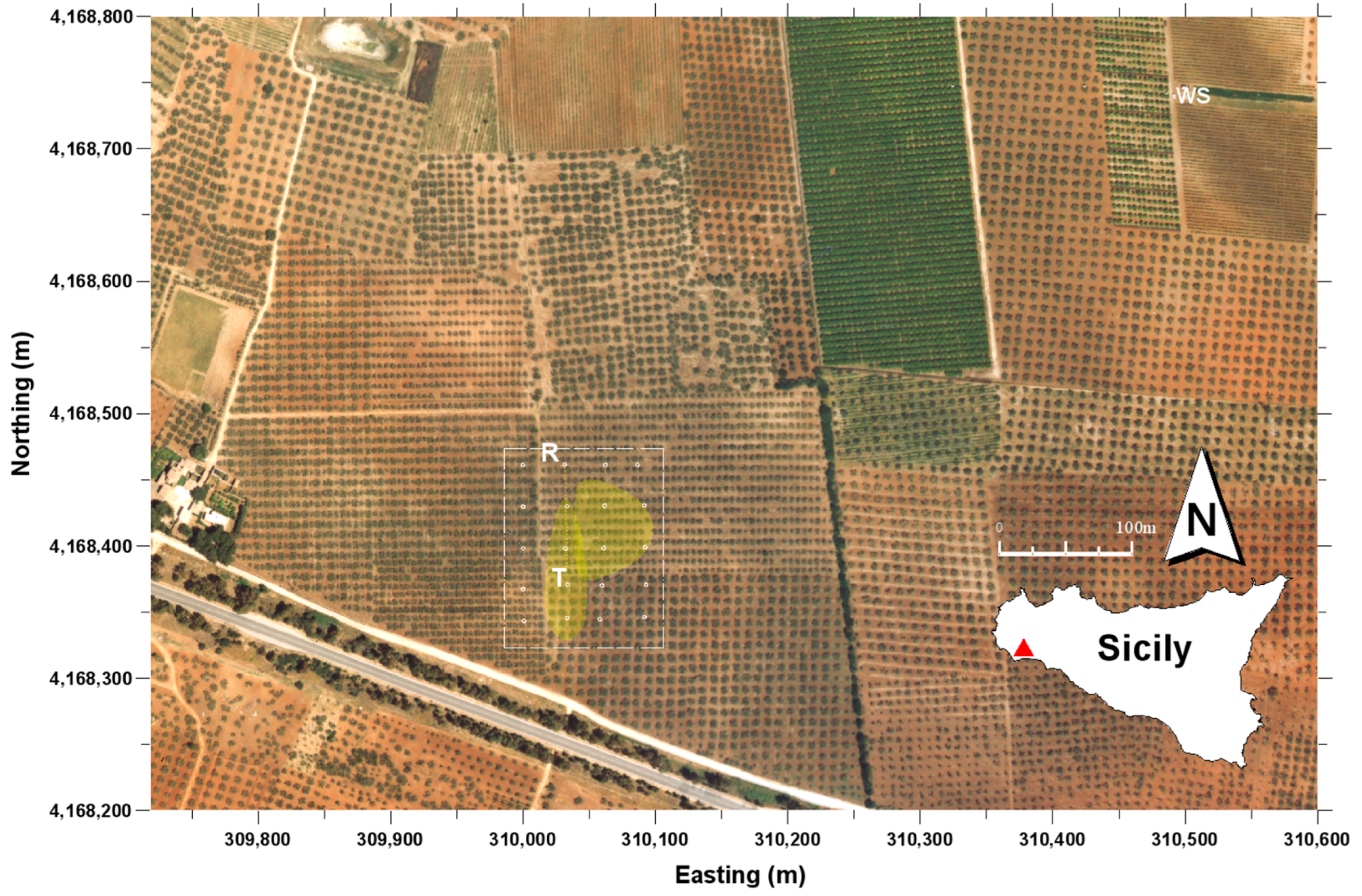
The study area (Figure 1) was located in the southwest of Sicily (Italy) next to the town of Castelvetrano (TP) on the commercial olive farm “Tenute Rocchetta” (Lat: 37°38′35″ N; Lon: 12°50′50″ E). The olive orchard (cv. Nocellara del Belice) has an extension of 13 ha and it is planted according to a regular grid of 8 m × 5 m (~250 trees/ha). The orchard is irrigated with a micro-irrigation system with drip laterals along the tree rows. Each lateral contains four 8 L/h emitters per tree, placed on both sides of each plant at a distance of one and two meters. The fraction of wetted soil after an irrigation event was generally equal to 0.2, while the fraction of canopy cover was about 0.3.
The experimental activities were conducted during two irrigation seasons in 2008 and 2009. The irrigation scheduling followed the ordinary management practised in the surrounding area [20]. In 2008, the total irrigation depth provided by the farmer was equal to 122 mm divided into four watering events, whereas in 2009 it resulted in 127 mm distributed into five events.
Previous research activities [3,12,14,21] on the farm have investigated different monitoring techniques for crop water requirements. These have been done at different spatial scales and acquisition platforms: ground-based sensing [3], micrometeorology [12,14], and remote sensing acquisitions [21]. During 2008, a scintillometric application [14] addressed quantifying crop water requirements at the field scale. This process validated an upscaling procedure of the tree fluxes based on measurements of the leaf area index by remote sensing.
Because the upscaling procedure [13] was calibrated with reference to the sensing surface (footprint) investigated by the scintillometer, our research used variables collected in a sampling area covering this sensing surface. In particular, according to a preliminary footprint analysis (Figure 1), sampling points for the physical analysis and bulk electrical conductivity measurements of the soil were chosen inside the area where the “relative normalized contribution” to actual evapotranspiration, ETr, was on average close to the daily maximum. The footprint reference area was marked by considering the wind direction acting along and perpendicular to the scintillometer path in order to be sure that the location of the source area was always inside the sampling grid (Figure 1).
The soil’s electrical conductivity and texture and bulk electrical conductivity were evaluated on a surface of 1.25 ha in which 20 measurements were selected according to a 25 m × 25 m square grid. In each point, soil texture analysis and six EM38 measurements (three with horizontal and three with a vertical dipole) were collected. The EM38 sensor was in particular placed at ground level and (i) at the center of four trees, (ii) in the middle between two trees along the row and (iii) below an emitter.
In 2008, an irrigation event of about 33 mm distributed over two days was monitored with EM38, while in 2009 two events were observed. For each wetting event, EM38 measurements were executed immediately before and after irrigation until the following watering based on a weekly time-step. Furthermore, additional measurements of soil water status were collected during and after rain events.
2.1. Soil Physical Characterization and EM38 Calibration Procedure
A preliminary analysis determined the soil salinity on sieved soil randomly collected in the topsoil (0–0.3 m). Soil electrical conductivity was determined on 1:5 soil-water extract with a conductivity meter (microCM 2200, Crison Instruments, Barcelona, Spain) by a standard procedure [22]. These results showed the absence of salt accumulation since the electrical conductivity ranged from 0.11 to 0.36 dS m−1 [23].
A texture analysis was performed on the soil samples collected on the grid to determine the spatial variability of the clay content in the area. At each sampling point, around 1 kg of topsoil (0–0.3 m) was collected and the sample positions (Universal Transverse Mercator, UTM, coordinates system) detected with a differential GPS (Global Positioning System). The textural distribution of the soil samples was determined in the laboratory by the hydrometer method. The percentage of clay content (diameter lower than 2 μm) was used as a proxy variable to investigate the spatial variability of both the EM38 response and the fraction of transpirable soil water (FTSW).
Due to the considerable variability of the soil clay content, two sites (A and B) were selected to calibrate the EM38 sensor. At each site, a more detailed soil textural analysis was carried out on disturbed soil samples collected every 0.15 m up to 1.2 m depth. After analyzing each sample, the data was aggregated in layers of 0.3 m depth. At each site, a Diviner 2000 access tube, 1.2 m long, was installed. This technique permitted pairing the measurements of soil bulk electrical conductivity and SWC along the soil profile. The Diviner 2000 [16] is a handheld monitoring device for soil water content. It consists of a portable display/logger unit connected to an automatic depth-sensing probe in which two electric rings, forming a capacitor, are installed at its extremity. The capacitor and the oscillator represent a circuit that generates an oscillating electrical field into the soil through the wall of the access tube. Consequently, the sensor’s output is represented by the resonant frequency of the circuit (raw count) that depends on the dielectric properties of the soil surrounding the access tube. The resonant frequency detected by the sensor in the soil (Fs) is scaled to a value, SF, ranging between 0 and 1 on the basis of the frequency readings obtained in air (Fa) and water (Fw). At the same time, the site-specific calibration equations proposed by Provenzano et al. [17] were used to transform the scaled frequency measured by the Diviner 2000 probe and to obtain accurate SWC estimations for the investigated sites.
The EM38 sensor (Geonics Ltd., Mississauga, ON, Canada) consists of a transmitter and a receiver coil, installed 1.0 m apart at the opposite ends of a bar, and operating at a frequency of 14.6 kHz. The investigated depth range depends on the coil configuration, as well as on the distance between coils [24]. While the distance is fixed, the coils can be oriented in a vertical mode with the magnetic dipole maintained perpendicular to the soil surface, or in a horizontal mode with the dipole parallel to the soil surface. In the horizontal mode, the highest sensitivity is at the soil surface, while in the vertical mode the maximum is approximately 0.3–0.4 m below the instrument. The measurement unit of the bulk electrical conductivity (EC) is in milliSiemens per meter (mS m−1).
The calibration procedure was carried out during the irrigation season of 2008. It was based on 47 profiles of soil water content and contextual readings of the soil bulk electrical conductivity in the vertical (ECV) and horizontal (ECH) dipole orientations. EM38 measurements were acquired around the Diviner 2000 access tubes in different periods to explore at both sites a wide range of soil water status conditions.
The EM38 was calibrated and nulled according to the manufacturer’s instruction before each measurement. Vertical (ECV) and horizontal (ECH) readings were weighted in order to obtain a single value of the total soil electrical conductivity (ECt) as suggested by Cook and Walker [25]. A linear combination of vertical and horizontal readings was particularly used to assess a single depth response function that better matches the portion of the investigated soil profile (ECt):
Following the approach suggested by Lacape et al. [4], at each site the total transpirable soil water (TTSW) was calculated by summing the differences over the explored soil depth (1.2 m) between the soil water content at field capacity (SWCfc) (upper limit) and the minimum soil water content (SWCmin) (lower limit):
In addition, the available soil water at a given time (ASW) was calculated by summing the differences between the actual (SWCd) and minimum (SWCmin) soil water content over the same soil depth:
Soil water content at a field capacity (SWCfc), as well as the lower limit (SWCmin), was directly obtained by examining the temporal dynamics of SWC along the soil profile, following the assumptions of Polak et al. [8]. Immediately after a wetting event, a sharp decrease in SWC occurs, mainly due to the free drainage in which the root water uptake can be neglected. After that, the reductions in SWC are due to the combination of free drainage and root water uptake. This takes place until a period in which free drainage ceases and SWC reaches its minimum (SWCmin). Below this value, the roots cannot extract more water from the soil [4].
As suggested by Polak et al. [8], SWC can be considered “close to” field capacity (SWCfc) when most of the free water has drained. In irrigation science, this value is considered the upper limit of available soil water, while, as suggested by Lacape et al. [4], SWCmin can be placed instead of the ordinary wilting point.
2.2. Transpiration Fluxes and Relative Transpiration Measurements
The standard meteorological variables were provided by the SIAS (Servizio Informativo Agrometeorologico Siciliano) weather station n. 302, located about 500 m northeast of the experimental site (Figure 1). The weather station is equipped with sensors for hourly measurements of air temperature at a 2-m height, precipitation, relative air humidity, wind speed and direction at 2- and 10-m heights, air pressure, and global incoming solar radiation. The net radiation R and its components were measured with a four-component net radiometer (NR01, Hukeseflux, Delft, The Netherlands).
The macroscopic approach was used to quantify the water status of the olive trees, defined as a reduction term (α) of maximum crop transpiration:
where Ta and Tp are the actual and maximum transpiration, respectively. Once the latter is determined, the knowledge of α allows the estimation of actual transpiration Ta. The maximum transpiration (Tp), was estimated by following the procedure suggested by Jarvis and McNaughton [26]:
where Δ (kPa C−1) is the slope of the saturation vapor pressure curve, R (W m−2) is the net radiation, ρ (Kg m−3) is the air density, Cp (J Kg−1 K−1) is the air specific heat at constant pressure, γ (kPa K−1) is the psychometric constant, VPD (kPa) is the air vapor pressure deficit, λ (J Kg−1) is the latent heat of vaporization, and ra and rc,min are the aerodynamic and the minimum canopy resistance (s m−1), respectively. All the variables in Equation (5) were obtained from the recorded meteorological data, except ra and rc, determined as indicated in Rallo and Provenzano [3].
The actual transpiration Ta was measured hourly on three olive trees by using two standard thermal dissipation probes (TDPs) [27] per tree. These trees were chosen based on a preliminary biometric analysis addressed to quantify the spatial distribution of leaf area index (LAI) in the study area. The measurements of LAI were performed with the LAI 2000 (Li-Cor Inc., Lincoln, NE, USA) by following a standard protocol for tree crops [28]. Considering that LAI was distributed according to a normal distribution with average µ = 1.55 m2 m−2 and standard deviation σ = ±0.4, trees with LAI between µ − σ and µ + σ were chosen to install the TDPs. At the end of the experiments, the sapwood area was determined by a colorimetric method on a total of six wood cores extracted with a Pressler gimlet from the same three trees and between each couple of sap flow probes.
Daily values of actual transpiration were obtained by integrating the instantaneous sap flux, following the hypothesis of neglecting tree capacitance. Daily transpiration depth (mm day−1) was obtained by dividing the daily flux (L day−1) for the pertinence area of the plant, equal to 40 m2.
Afterwards, to evaluate a representative value of the stand transpiration for the entire field, it was necessary to upscale the plant fluxes. This was done by considering, as a proximal variable, the ratio between the average leaf area index (LAIfield) and the value (LAIplant) measured on the plant in which sap fluxes were monitored. The up-scaling factor for each plant was derived by the remotely sensed LAI maps, as described in Cammalleri et al. [13], and validated by comparison with micrometeorological observed data [13,21].
2.3. Data Analysis and Pre-Processing
In 2008, a calibration model to estimate indirectly FTSW in the soil profile (1–2 m depth) was derived from the paired FDR and EM38 measurements. The ECV and ECH values were used to obtain the total electrical conductivity, ECt (Equation (1)). The root mean square error (RMSE) was used to quantify the performance of the relationship between FTSW and ECt.
A geostatistical analysis allowed the spatialization of both the clay content and the FTSW by means of ordinary Kriging [29].
Meteorological and sap flow data were pre-processed in order to create a database of daily values of maximum crop transpiration Tp, actual transpiration Ta, and relative transpiration α. During 2008, the Ta dataset comprehended the period from the first decade of June, corresponding to the initial fruit development stage, to the first decade of September, at the crop maturity stage.
XLSTAT statistical software and data analysis (Addinsoft XLSTAT, Paris, France) was used for the relationship between FTSW and relative transpiration α. Each α value was plotted as a function of the average value of FTSW retrieved on the corresponding day. The threshold at which the relative transpiration begins to decline was determined by using a logistic regression analysis, as described in [30].
3. Results and Discussion
3.1. Soil Surface Texture and Spatial Analysis
High variability of clay content was observed in the investigated area with values ranging between 15% and 40%. Sand content, on the other hand, was characterized by a maximum of 75% and a minimum of 41%. According to the USDA (United States Department of Agriculture) classification, the most frequent textural classes are represented by sandy-clay-loam and clay-loam (Figure 2).
The Kriging analysis of the spatialized clay content data showed a linear variogram and, consequently, it did not present range and sill parameters. However, a nugget variance effect (nugget = 17.8) was observed, which is imputable to measurement errors and/or to spatial sources of variation at distances smaller than the sampling interval. Thus, Figure 3 shows the map of measured clay percentage. As it can be observed, the coarsest texture (clay ≤ 20%) is mainly located in the southwest side of the study area.
According to the wide variability of soil clay content, two Diviner 2000 access tubes were installed in the NE (site A) and SW (site B) sides of the field. At both sites, the EM38 sensor had been preliminarily calibrated. Moreover, a detailed soil textural analysis was performed on disturbed soil samples collected every 0.15 m, up to 1.2 m depth. Table 1 shows the vertical distribution of clay content on layers of 0.3 m depth for sites A and B. Each value was obtained as the average of two measurements from each 0.15 m depth layer.
As it can be observed, site A is characterized by higher clay content than site B at all depths. Moreover, the percentage of clay decreased with soil depth in site A, whereas site B was more uniform.
3.2. Evaluation of Total Transpirable Soil Water (TTSW)
A wide range of soil water content was considered for calibrating the EM38 sensor. Figure 4 shows the maximum profiles, the average and the minimum SWC. The variability of SWC at site A was more marked than at site B due to the higher clay content. Additionally, the variability in the soil water content along the profile ensured that the collected dataset encompassed most of the soil water status occurring during the investigated irrigation season.
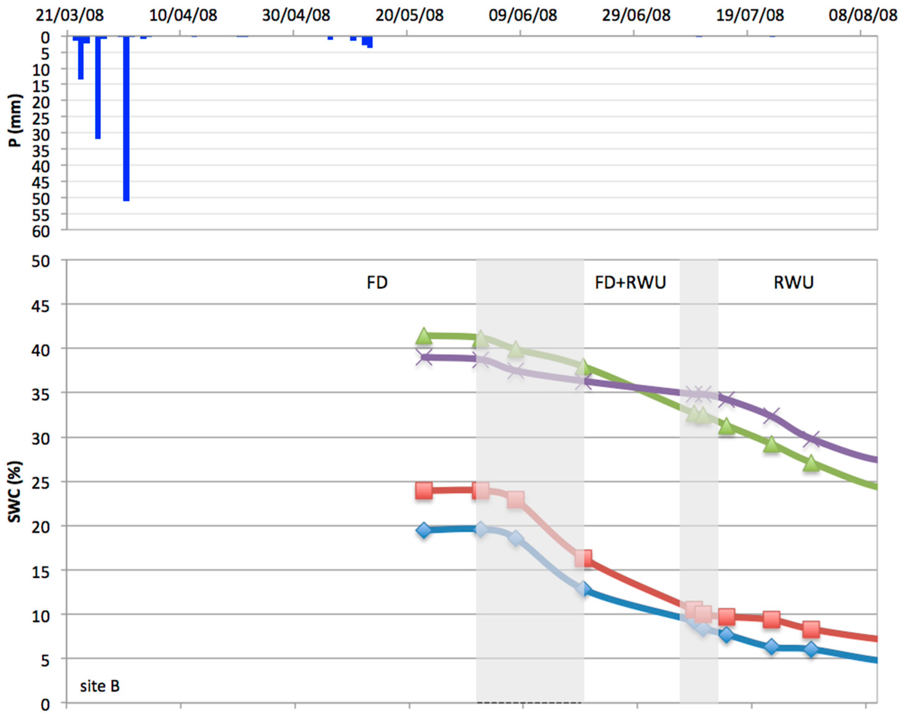
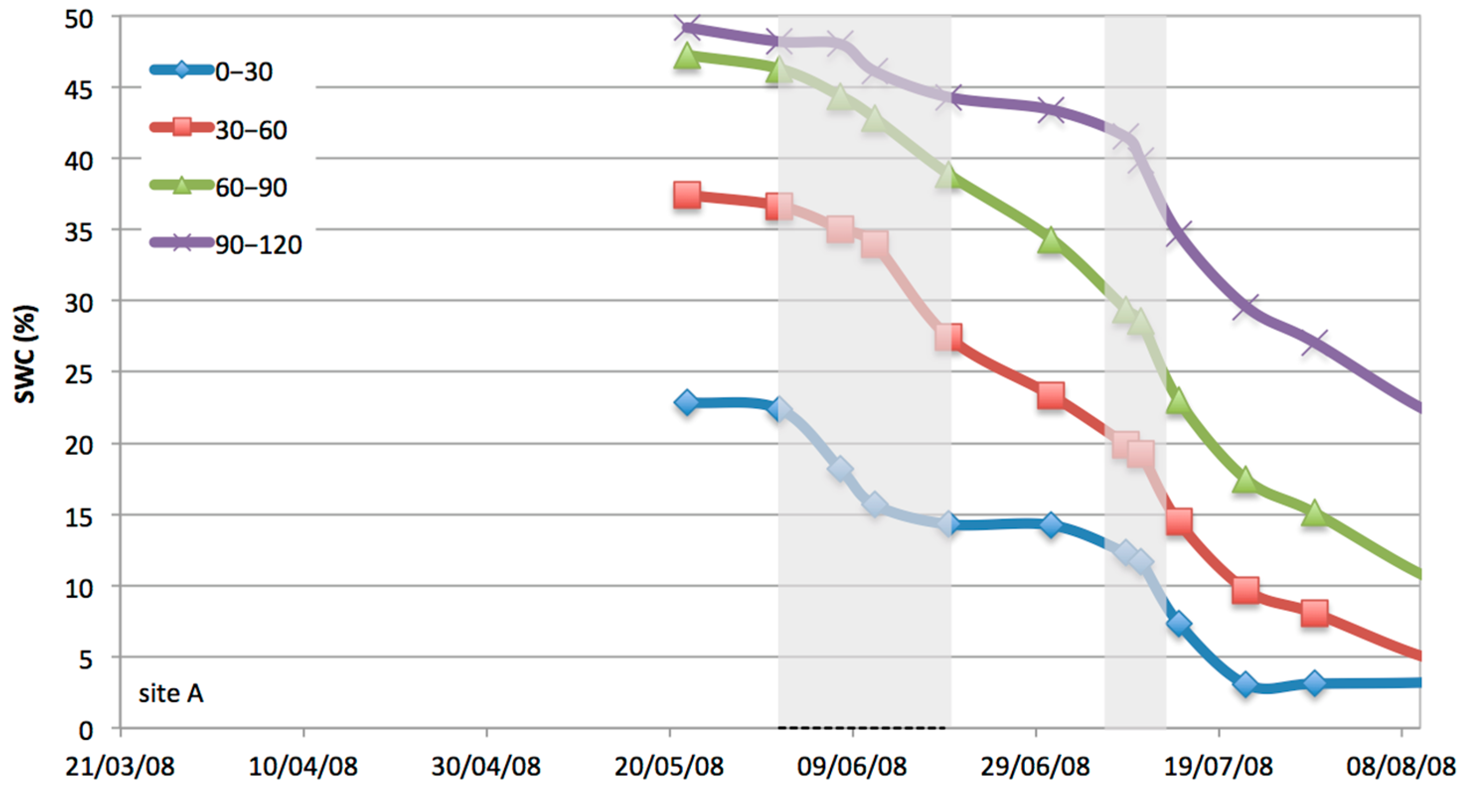
Figure 5 displays the temporal dynamics of the measured SWCs for sites A and B, respectively, during the 2008 irrigation season. In the same graphs, the transitory of SWCs among the three stages described by Polak et al. [8] are also shown. Measurements were collected from May 20th, about 10 days after the rainy events registered in the first decade of the month. According to the low transpiration activity and the limited rainfall of the period, it is plausible to hypothesize that the initial SWCs were acquired in the absence of free drainage when only root water uptake occurred. In agreement with Polak and Wallach [8], this SWC corresponds to the field capacity of the layer. Practically, we considered SWCfc as the average value of SWC data collected from 1 June to 19 June.
The analysis of SWC acquired over the whole season allowed, as well, the evaluation of the minimum soil water content SWCmin.
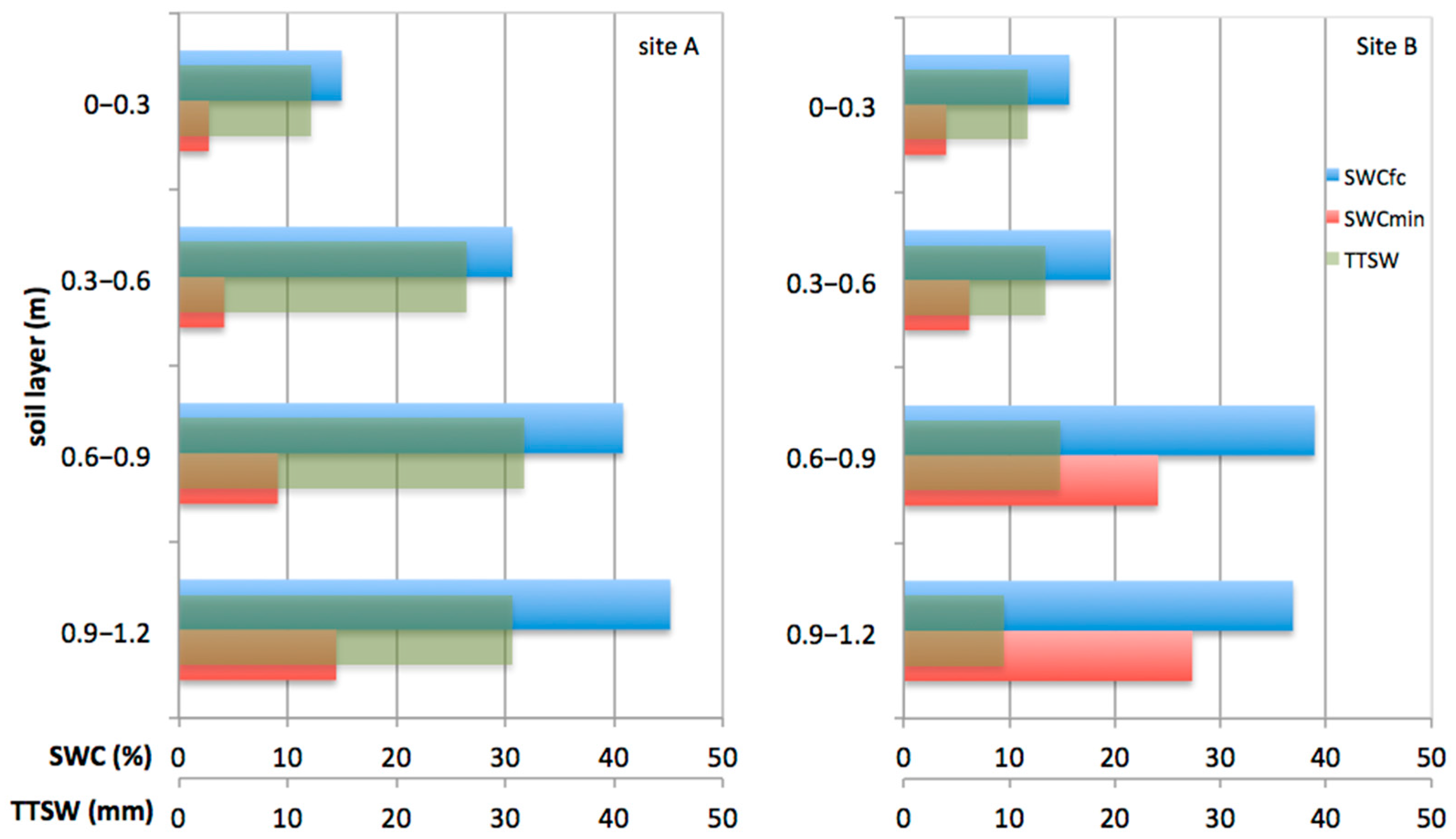
Based on the above-mentioned analysis, the upper (SWCfc) and the lower (SWCmin) limits used to evaluate TTSW were obtained for both sites at the investigated soil layers. Figure 6 shows the values of SWCfc and SWCmin for the four soil layers, as well as the corresponding TTSW.
When considering the upper soil layer (0–0.3 m), TTSW values were similar at sites A and B, whereas these values were higher at site A than at B when the higher depths are considered. The SWCmin at A was lower than at B for all investigated depths while, on the contrary, the SWCfc was generally higher. These limits depend on soil texture, as well as on the root water uptake ability [9]. At both sites, the differences in TTSW were consistent with the recognized soil textures.
3.3. EM38 Model to Predict the Fraction of Transpirable Soil Water
As illustrated in Figure 7, a strong correlation was observed between ECt measured with EM38 and the corresponding FTSW values obtained with the Diviner 2000 measurements. Experimental FTSW and ECt data obtained at sites A and B were linearly correlated with R2 and RMSE equal to 0.86 and 0.10, respectively.
Huth and Poulton obtained similar results [19], which evidenced that the term SWCmin used to evaluate FTSW accounts for the electrical conductivity of the solid phase. Consequently, it reduces the effects of the different clay content that characterizes these two sites. Even the term SWCd-SWCmin accounts for the effects of both the electrical conductivity of the liquid phase and of the soil pore space.
3.4. Temporal and Spatial Variability of Soil Bulk Electrical Conductivity and Plant Water Status
Figure 8 depicts the temporal dynamics of the soil bulk electrical conductivity ECt measured with the EM38 sensor during the irrigation seasons of 2008 and 2009, as well as the irrigation and precipitation events occurring in the examined periods. As it can be observed, the temporal dynamics of ECt are sensible to changes in the soil water status. In fact, ECt values increased after the wetting events and decreased during soil drying processes.
Even the standard deviation associated with ECt was higher after irrigation and lower when the soil was dry. This higher standard deviation observed after irrigation events is mainly due to the localized irrigation system. In fact, EM38 readings, collected at the center of four trees, did not detect any change in soil water content, contrary to the readings collected below the emitters.
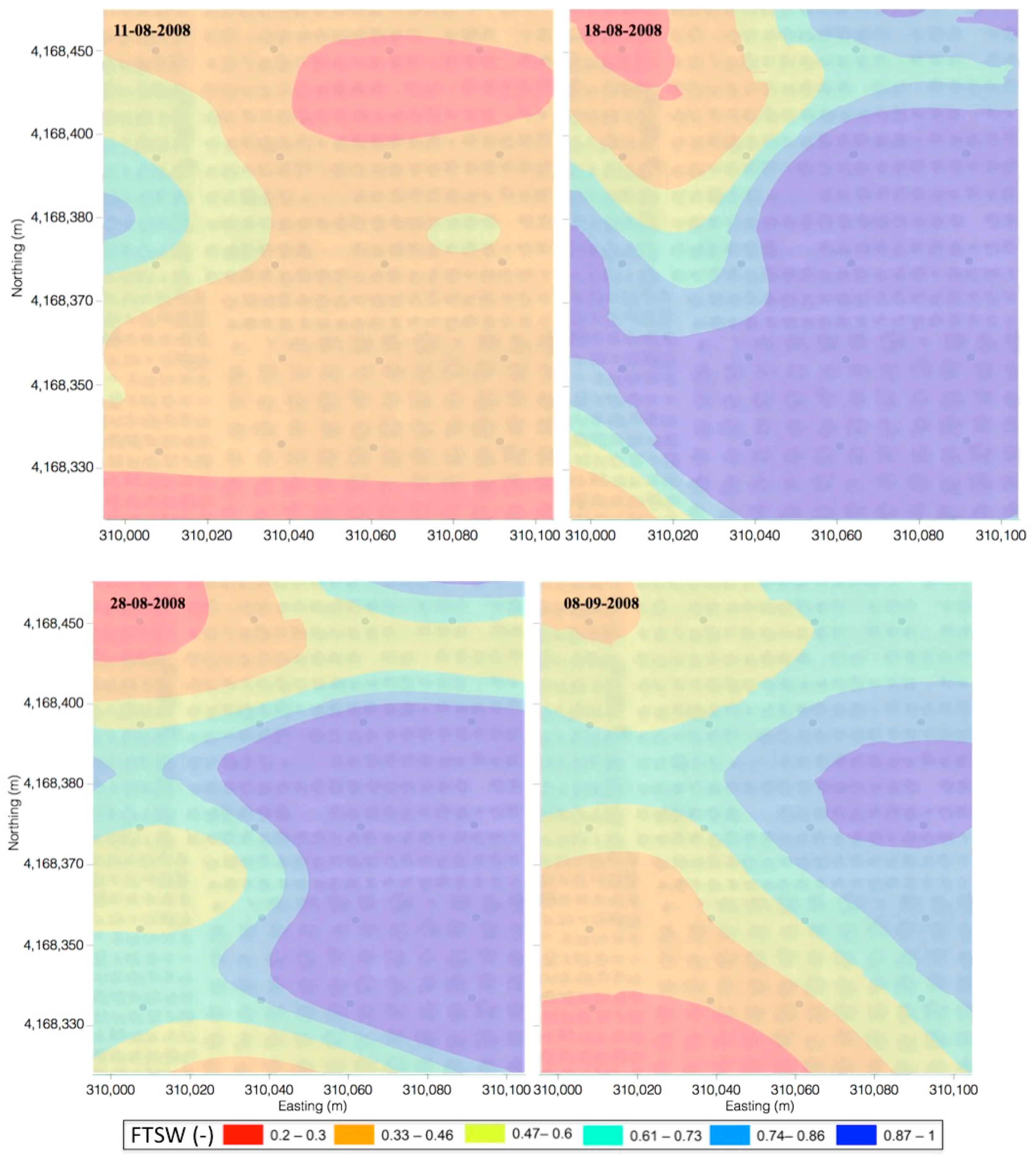
Relative to the 2008 season, the spatiotemporal variability of FTSW values was investigated before and after the irrigation event of 14 August. Figure 9 shows for some of these days the spatial distributions of FTSW indirectly estimated on the basis of the EM38 survey. In the same manner, more structured patterns occurred after irrigation as a possible consequence of subsurface flow, soil evaporation, and root water uptake processes. It is possible to assume that the combination of these hydrological processes affects the soil bulk electrical conductivity and therefore the fraction of water available to the plants.
According to the spatial variability of the soil texture (Figure 3), the fastest drying processes occurred in the east side of the area where the sand percentage is relatively higher. On the other hand, the west side, characterized by clay percentages higher than 30–35%, showed high values of FTSW even one month after irrigation.
3.5. Relations between Relative Transpiration and the Fraction of Transpirable Soil Water
Figure 10 displays the values of measured relative transpiration (α) as a function of the fraction of transpirable soil water (FTSW) estimated in 2008 and 2009. Moreover, this figure performs the logistic model used to fit the experimental data. As it can be observed for any fixed FTSW, the variability of the corresponding α depends on the atmospheric water demand [3]. Despite the limited number of measurements related to the high water content, the values of the relative transpiration, α, were practically constant when the soil water content was higher than a threshold, below which it decreased drastically. The statistical analysis evidenced a critical threshold of FTSW, approximately equal to 0.38, below which the reduction of relative transpiration is recognizable.
A more detailed analysis of the data evidenced that, despite a large variability of α, the corresponding changes of FTSW were almost limited. Relative transpiration was more or less constant and equal approximately to 1 for a higher FTSW than the critical value, whereas the measured relative transpiration dropped off to a minimum value of about 0.5 for lower FTSW.
Unfortunately, the absence of Ta Tp−1 measurements lower than 0.5 did not permit to clearly identify the best shape of the curve under more severe water stress conditions than those observed. In fact, it was very difficult to reach α values lower than 0.5 for the examined situation, considering that (i) the high capacitance characterizing the olive plants allows a certain adaptation to water stress conditions; (ii) the investigated field is characterized by high values of soil water retention; and (iii) due to the relatively high plant spacing a large soil volume is available for root water uptake.
4. Conclusions
The measurements acquired in an olive orchard with the EM38 ground conductivity meter (Geonics Ltd., Mississauga, ON, Canada) combined with Diviner 2000 probe (Sentek Pty Ltd., Stepney, Australia) can provide quick and suitable monitoring of the fraction of transpirable soil water (FTSW). Moreover, the relationship between FTSW and the relative transpiration, α, was assessed based on the values of actual crop transpiration, Ta. These data were measured with sap-flow sensors and up-scaled through the leaf area index (LAI).
A strong linear relationship (R2 = 0.86) was found between the fraction of transpirable soil water (FTSW), integrated to a depth of 1.2 m, and the total bulk electrical conductivity (ECt). This last value was obtained by combining EM38 readings at the soil surface in the vertical and horizontal dipole orientations. Despite the different soil clay content characterizing the area, a single model was found to describe the variability of FTSW with ECt. These results are in line with those of other authors who evidenced that the term SWCmin, used to evaluate FTSW, accounts for the conductivity of the solid phase. Consequently, it reduces the effects of the different clay contents characterizing the investigated sites.
More structured patterns of FTSW occurred after the irrigation events because of the occurrence of water redistribution, soil evaporation, and root water uptake processes. The high standard deviation, mainly observed after irrigation, was due to the localized irrigation system. This water distribution method determines extensive gradients of soil water content around the trees and through the soil depth.
In fact, EM38 readings collected at the center of four trees did not detect any change in soil water content, contrary to the readings collected below emitters. Therefore, to account for the large variability in root density and water uptake in arboreal crop systems, it is necessary to increase the temporal frequency of acquisition, as well as the number of spatial acquisitions. This procedure could be faced by means of a vehicular-based sampling.
The macroscopic approach was followed to assess the empirical function able to describe the plant water status response and to correlate the relative transpiration to the FTSW. Despite the limited number of measurements, a value of FTSW = 0.38 was found as a critical threshold below which a strong reduction of relative transpiration can be recognized.
The research indicates the effectiveness of EMI techniques in monitoring the variations of soil water content in response to irrigation and root water uptake. This technique allows a great degree of flexibility in terms of spatial and temporal sampling resolution. This is possible mainly when precise knowledge of the vertical distribution of soil water content is not as important as its variation in time and space. The availability for using FDR measurements to calibrate EMI acquisitions in areas characterized by different soil properties has concrete advantages, even in precision agriculture, when accurate monitoring of soil water content is necessary. Furthermore, once performed, a suitable α = f(FTSW) model for actual field transpiration fluxes could be determined by multiplying the maximum crop transpiration to the relative transpiration coefficient estimated by the proposed methodology. Further research will be carried out to extend the domain of explored FTSW values, and with a more detailed scheme of sampling.
Acknowledgments
Data analyses have been partly funded by the Università di Pisa (Fondi di Ateneo, 2016) and MIUR (Finanziamento delle attività base di ricerca, 2017-Rallo). Experimental data were collected in the frame of research projects co-financed by the University of Palermo.
Author Contributions
G.R. and G.P. designed the experimental layout and analyzed the data. Field experiments were carried out by G.R. All authors contributed to the final editing of the manuscript.
Conflicts of Interest
The authors declare no conflict of interest. The founding sponsors had no role in the design of the study; in the collection, analyses, or interpretation of data; in the writing of the manuscript; or in the decision to publish the results.
References
- Costantini, E.A.C.; Pellegrini, S.; Bucelli, P.; Storchi, P.; Vignozzi, N.; Barbetti, R.; Campagnolo, S. Relevance of the Lin’s and Host hydropedological models to predict grape yield and wine quality. Hydrol. Earth Syst. Sci. 2009, 13, 1635–1648. [Google Scholar] [CrossRef]
- Xiloyannis, C.; Dichio, B.; Nuzzo, V.; Celano, G. Defence strategies of olive against water stress. Acta Hortic. 1999, 474, 423–426. [Google Scholar] [CrossRef]
- Rallo, G.; Provenzano, G. Modelling eco-physiological response of table olive trees (Olea europaea L.) to soil water deficit conditions. Agric. Water Manag. 2013, 120, 79–88. [Google Scholar] [CrossRef] [Green Version]
- Lacape, M.J.; Wery, J.; Annerose, D.J.M. Relationships between plant and soil water status in five field-grown cotton (Gossypium hirsutum L.) cultivars. Field Crop. Res. 1998, 57, 29–43. [Google Scholar] [CrossRef]
- Lecoeur, J.; Guilioni, L. Rate of leaf production in response to soil water deficits in field pea. Field Crop. Res. 1998, 57, 319–328. [Google Scholar] [CrossRef]
- Wery, J.; Lecoeur, J. Learning crop physiology from the development of a crop simulation model. J. Nat. Resour. Life Sci. Educ. 2000, 29, 1–7. [Google Scholar]
- Sinclair, T.; Ludlow, M. Influence of Soil Water Supply on the Plant Water Balance of Four Tropical Grain Legumes. Aust. J. Plant Physiol. 1986, 13, 329–341. [Google Scholar] [CrossRef]
- Polak, A.; Wallach, R. Analysis of soil moisture variations in an irrigated orchard root zone. Plant Soil 2001, 233, 145–159. [Google Scholar] [CrossRef]
- Cabelguenne, M.; Debaeke, P. Experimental determination and modelling of the soil water extraction capacities of crops of maize, sunflower, soya bean, sorghum and wheat. Plant Soil 1998, 202, 175–192. [Google Scholar] [CrossRef]
- Trambouze, W.; Voltz, M. Measurement and modelling of the transpiration of a Mediterranean vineyard. Agric. For. Meteorol. 2001, 107, 153–166. [Google Scholar] [CrossRef]
- Rallo, G.; Agnese, C.; Blanda, F.; Minacapilli, M.; Provenzano, G. Agro-Hydrological models to schedule irrigation of Mediterranean tree crops. Ital. J. Agrometeorol. 2010, 1, 11–21. [Google Scholar]
- Motisi, A.; Consoli, S.; Papa, R.; Cammalleri, C.; Rossi, F.; Minacapilli, M.; Rallo, G. Eddy covariance and sap flow measurement of energy and mass exchanges of woody crops in a Mediterranean environment. Acta Hortic. 2012, 951, 121–127. [Google Scholar] [CrossRef]
- Cammalleri, C.; Rallo, G.; Agnese, C.; Ciraolo, G.; Minacapilli, M.; Provenzano, G. Combined use of eddy covariance and sap flow techniques for partition of et fluxes and water stress assessment in an irrigated olive orchard. Agric. Water Manag. 2013, 120, 89–97. [Google Scholar] [CrossRef] [Green Version]
- Cammalleri, C.; Agnese, C.; Ciraolo, G.; Minacapilli, M.; Provenzano, G.; Rallo, G. Actual evapotranspiration assessment by means of a coupled energy/hydrologic balance model: Validation over an olive grove by means of scintillometry and measurements of soil water contents. J. Hydrol. 2010, 392, 70–82. [Google Scholar] [CrossRef]
- Starr, J.L.; Rowland, R. Soil Water Measurement Comparisons between Semi-Permanent and Portable Capacitance Probes. Soil Sci. Soc. Am. J. 2007, 71, 51–52. [Google Scholar] [CrossRef]
- Evett, S.R.; Tolk, J.A.; Howell, T.A. Soil Profile Water Content Determination: Sensor Accuracy, Axial Response, Calibration, Temperature Dependence, and Precision. Vadose Zone J. 2006, 5, 894–907. [Google Scholar] [CrossRef]
- Provenzano, G.; Rallo, G.; Ghazouani, H. Assessing Field and Laboratory Calibration Protocols for the Diviner 2000 Probe in a Range of Soils with Different Textures. J. Irrig. Drain. Eng. 2016, 142, 4015040. [Google Scholar] [CrossRef]
- Corwin, D.L.; Plant, R.E. Applications of apparent soil electrical conductivity in precision agriculture. Comput. Electron. Agric. 2005, 46, 1–10. [Google Scholar] [CrossRef]
- Huth, N.I.; Poulton, P.L. An electromagnetic induction method for monitoring variation in soil moisture in agroforestry systems. Aust. J. Soil Res. 2007, 45, 63–72. [Google Scholar] [CrossRef]
- Rallo, G.; Agnese, C.; Minacapilli, M.; Provenzano, G. Comparison of SWAP and FAO agro-hydrological models to schedule irrigation of wine grapes. J. Irrig. Drain. Eng. 2012, 138, 581–591. [Google Scholar] [CrossRef]
- Cammalleri, C.; Ciraolo, G.; Minacapilli, M.; Rallo, G. Evapotranspiration from an Olive Orchard using Remote Sensing-Based Dual Crop Coefficient Approach. Water Resour. Manag. 2013, 27, 4877–4895. [Google Scholar] [CrossRef]
- Carter, M.R.; Gregorich, E.G.; Pennock, D.; Yates, T.; Braidek, J. Electrical Conductivity and Soluble Ions. In Soil Sampling and Methods of Analysis, 2nd ed.; CRC Press: Boca Raton, FL, USA, 2007; Volume 44, p. 3. [Google Scholar]
- Ditzler, C.; Scheffe, K.; Monger, H.C. Examination and Description of Soil Profiles. In Soil Survey Manual (SSM)–Soil Science Division Staff; USDA Handbook 18; Government Printing Office: Washington, DC, USA, 2017. Available online: https://www.nrcs.usda.gov/wps/portal/nrcs/detailfull/soils/ref/?cid=nrcs142p2_054262 (accessed on 21 January 2018).
- McNeill, J.D. Electromagnetic Terrain Conductivity Measurement at Low Induction Numbers; Technical Note TN-6; Geonics Ltd.: Mississauga, ON, Canada, 1980; p. 13. Available online: http://www.geonics.com/pdfs/technicalnotes/tn6.pdf (accessed on 21 January 2018).
- Cook, P.G.; Walker, G.R. Depth Profiles of Electrical Conductivity from Linear Combinations of Electromagnetic Induction Measurements. Soil Sci. Soc. Am. J. 1992, 56, 1015–1022. [Google Scholar] [CrossRef]
- Jarvis, P.G.; Mcnaughton, K.G. Stomatal Control of Transpiration: Scaling Up from Leaf to Region. Adv. Ecol. Res. 1986, 15, 1–49. [Google Scholar]
- Granier, A. Evaluation of transpiration in a Douglas-fir stand by means of sap flow measurements. Tree Physiol. 1987, 3, 309–320. [Google Scholar] [CrossRef] [PubMed]
- Villalobos, F.J.; Orgaz, F.; Mateos, L. Non-destructive measurement of leaf area in olive (Olea europaea L.) trees using a gap inversion method. Agric. For. Meteorol. 1995, 73, 29–42. [Google Scholar] [CrossRef]
- Jin, L.; Heap, A.D. A review of comparative studies of spatial interpolation methods in environmental sciences: Performance and impact factors. Ecol. Inform. 2011, 6, 228–241. [Google Scholar]
- Ahuja, L.R.; Reddy, V.R.; Saseendran, S.A.; Yu, Q. Response of Crops to Limited Water: Understanding and Modeling Water Stress Effects on Plant Growth Processes. In Advances in Agricultural Systems Modeling; American Society of Agronomy, Crop Science Society of America, Soil Science Society of America: Madison, WI, USA, 2008; Volume 11. [Google Scholar]
Figure 1.
Location of the experimental farm with the sampling zone (dashed box) and the measurement points (dots). Scintillometric footprints (yellow shaded area) along two wind directions are also indicated. WS: weather station; R: scintillometer receiver unit; T: scintillometer transmission unit.
Figure 1.
Location of the experimental farm with the sampling zone (dashed box) and the measurement points (dots). Scintillometric footprints (yellow shaded area) along two wind directions are also indicated. WS: weather station; R: scintillometer receiver unit; T: scintillometer transmission unit.

Figure 2.
USDA soil texture triangle and texture of topsoil samples collected at EM38 measurement points.
Figure 2.
USDA soil texture triangle and texture of topsoil samples collected at EM38 measurement points.
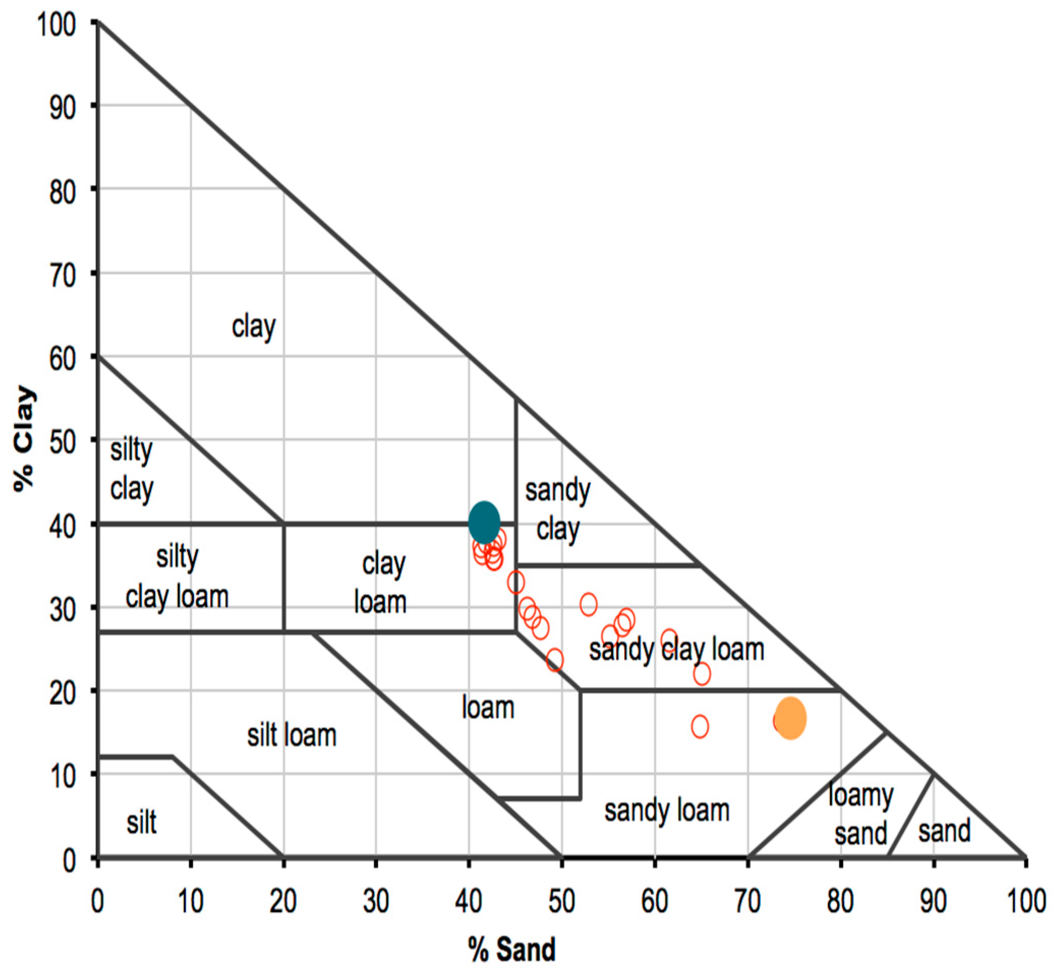
Figure 3.
Map of the topsoil clay percentage. North and East coordinates are referred to UTM ED50 system. The sampling points (dots) and a transparent image of the field are also shown.
Figure 3.
Map of the topsoil clay percentage. North and East coordinates are referred to UTM ED50 system. The sampling points (dots) and a transparent image of the field are also shown.
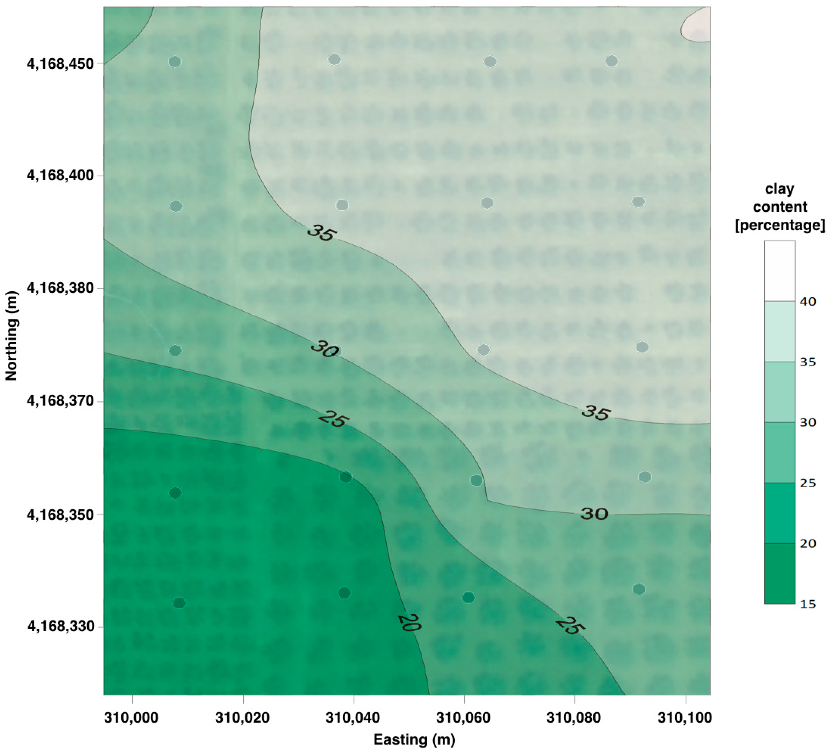
Figure 4.
Maximum, minimum, and average profiles of soil water content observed at A) sites A and B) site B.
Figure 4.
Maximum, minimum, and average profiles of soil water content observed at A) sites A and B) site B.
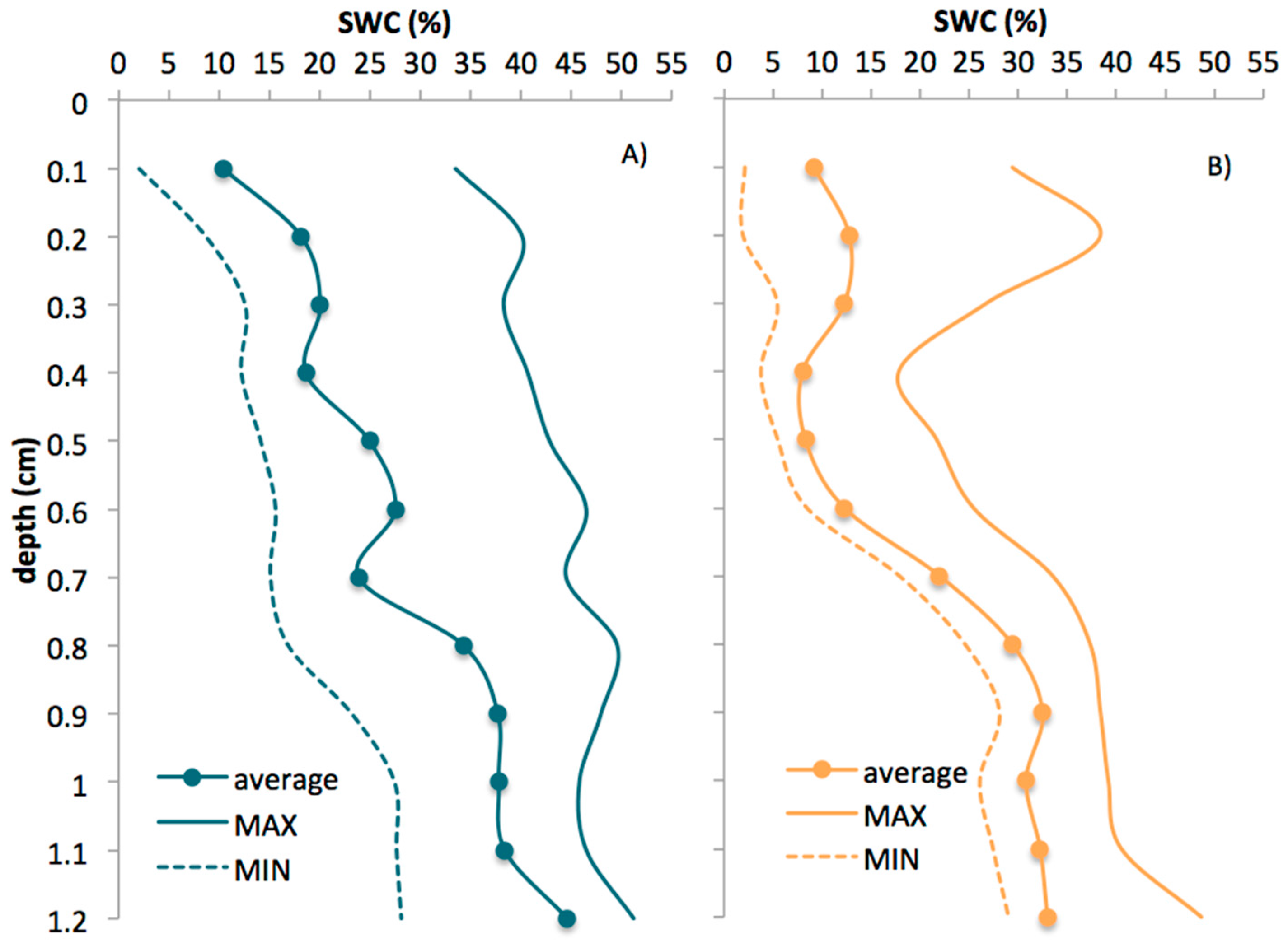
Figure 5.
Temporal dynamics of SWC observed at different soil layers at sites A and B. Shaded zones represent the transitory phases of SWCs between the stages of free drainage (FD), free drainage and root water uptake (FD + RWU), and root water uptake (RWU).
Figure 5.
Temporal dynamics of SWC observed at different soil layers at sites A and B. Shaded zones represent the transitory phases of SWCs between the stages of free drainage (FD), free drainage and root water uptake (FD + RWU), and root water uptake (RWU).


Figure 6.
Upper (SWCfc) and lower (SWCmin) limits of TTSW obtained for the four soil layers at sites A (left) and B (right).
Figure 6.
Upper (SWCfc) and lower (SWCmin) limits of TTSW obtained for the four soil layers at sites A (left) and B (right).

Figure 7.
Values of FTSW versus EM38 readings for sites A and B and their corresponding fitting equation.
Figure 7.
Values of FTSW versus EM38 readings for sites A and B and their corresponding fitting equation.
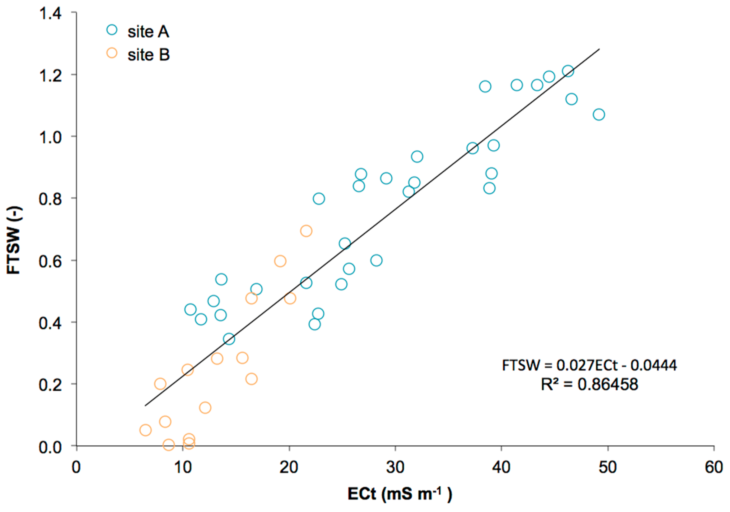
Figure 8.
Temporal dynamics of ECt values and the corresponding standard deviation during the irrigation seasons of 2008 and 2009. Irrigation and precipitation events are also represented.
Figure 8.
Temporal dynamics of ECt values and the corresponding standard deviation during the irrigation seasons of 2008 and 2009. Irrigation and precipitation events are also represented.
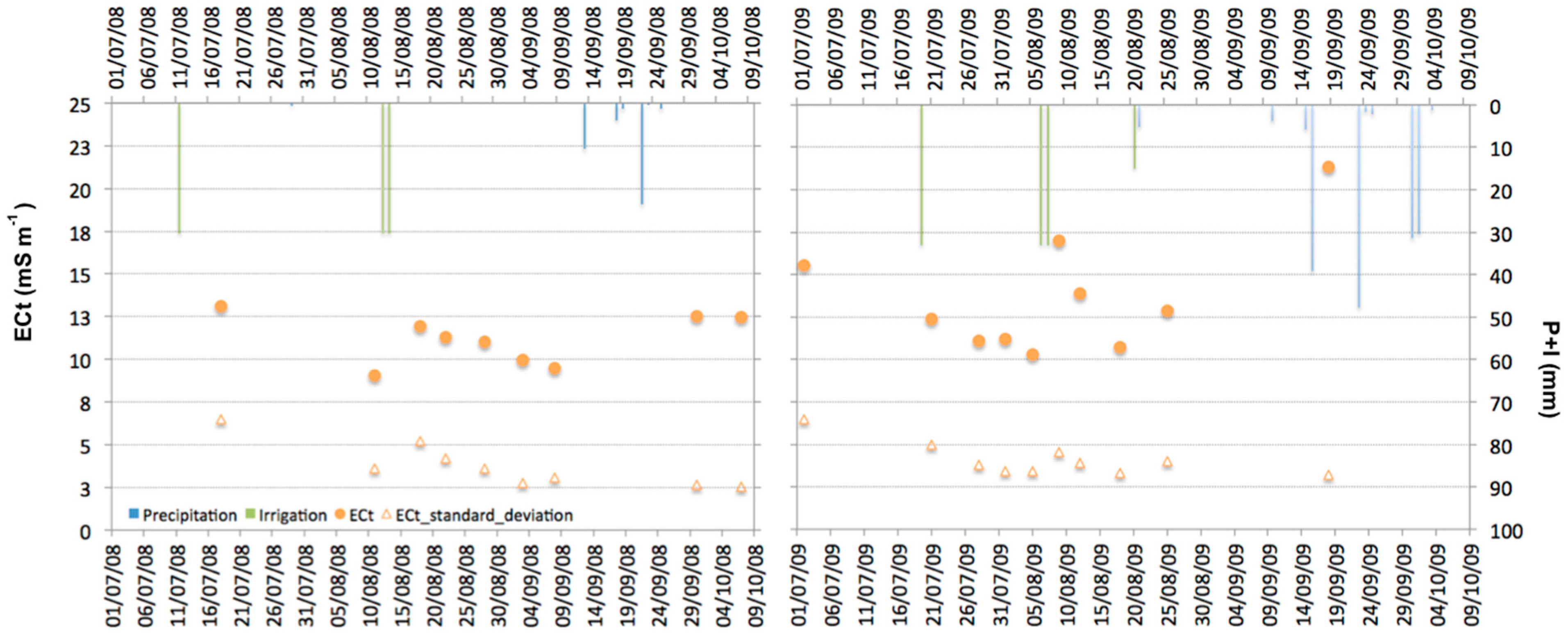
Figure 9.
Maps of transpirable soil water (FTSW) fraction before and after the irrigation event of 14 August 2008. The sampling points (dots) and the field image are also shown.
Figure 9.
Maps of transpirable soil water (FTSW) fraction before and after the irrigation event of 14 August 2008. The sampling points (dots) and the field image are also shown.

Figure 10.
Relationship between relative transpiration and the fraction of transpirable soil water.


Table 1.
Vertical distribution of clay percentages in sites A and B.
| Soil Layer (m) | Clay Content [%] | |
|---|---|---|
| Site A | Site B | |
| 0–0.3 | 42.4 | 28.4 |
| 0.3–0.6 | 43.3 | 27.8 |
| 0.6–0.9 | 39.1 | 27.3 |
| 0.9–1.2 | 27.9 | 26.0 |
© 2018 by the authors. Licensee MDPI, Basel, Switzerland. This article is an open access article distributed under the terms and conditions of the Creative Commons Attribution (CC BY) license (http://creativecommons.org/licenses/by/4.0/).
Share and Cite
MDPI and ACS Style
Rallo, G.; Provenzano, G.; Castellini, M.; Sirera, À.P. Application of EMI and FDR Sensors to Assess the Fraction of Transpirable Soil Water over an Olive Grove. Water 2018, 10, 168. https://doi.org/10.3390/w10020168
AMA Style
Rallo G, Provenzano G, Castellini M, Sirera ÀP. Application of EMI and FDR Sensors to Assess the Fraction of Transpirable Soil Water over an Olive Grove. Water. 2018; 10(2):168. https://doi.org/10.3390/w10020168
Chicago/Turabian StyleRallo, Giovanni, Giuseppe Provenzano, Mirko Castellini, and Àngela Puig Sirera. 2018. "Application of EMI and FDR Sensors to Assess the Fraction of Transpirable Soil Water over an Olive Grove" Water 10, no. 2: 168. https://doi.org/10.3390/w10020168
Note that from the first issue of 2016, this journal uses article numbers instead of page numbers. See further details here.