Powerful Software to Simulate Soil Consolidation Problems with Prefabricated Vertical Drains


Abstract
:1. Introduction
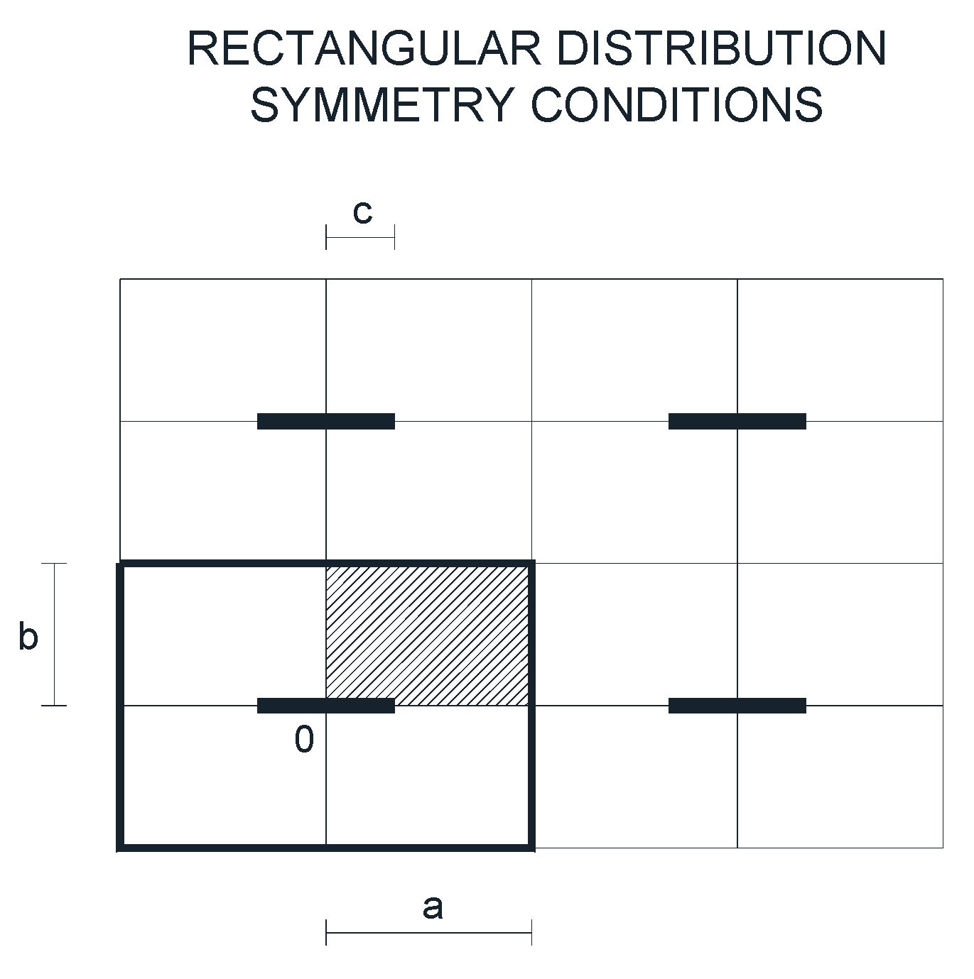
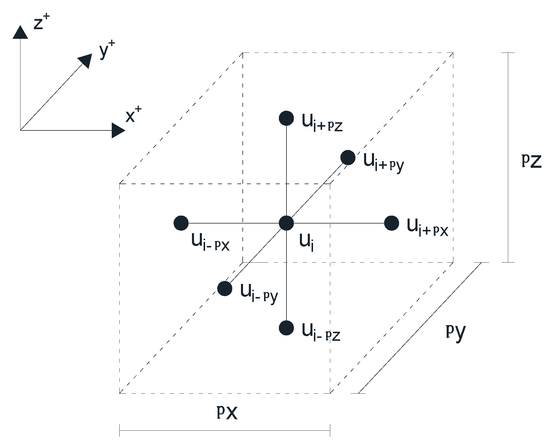
2. Fundamentals of Soil Consolidation with Prefabricated Vertical Drains and Network Model
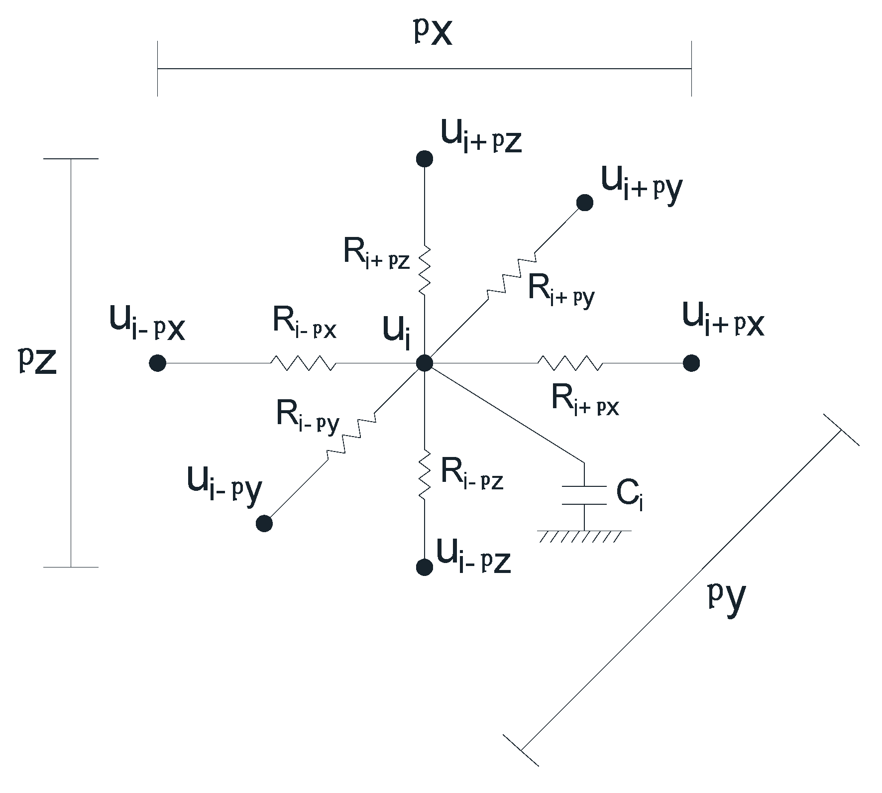
Network Model
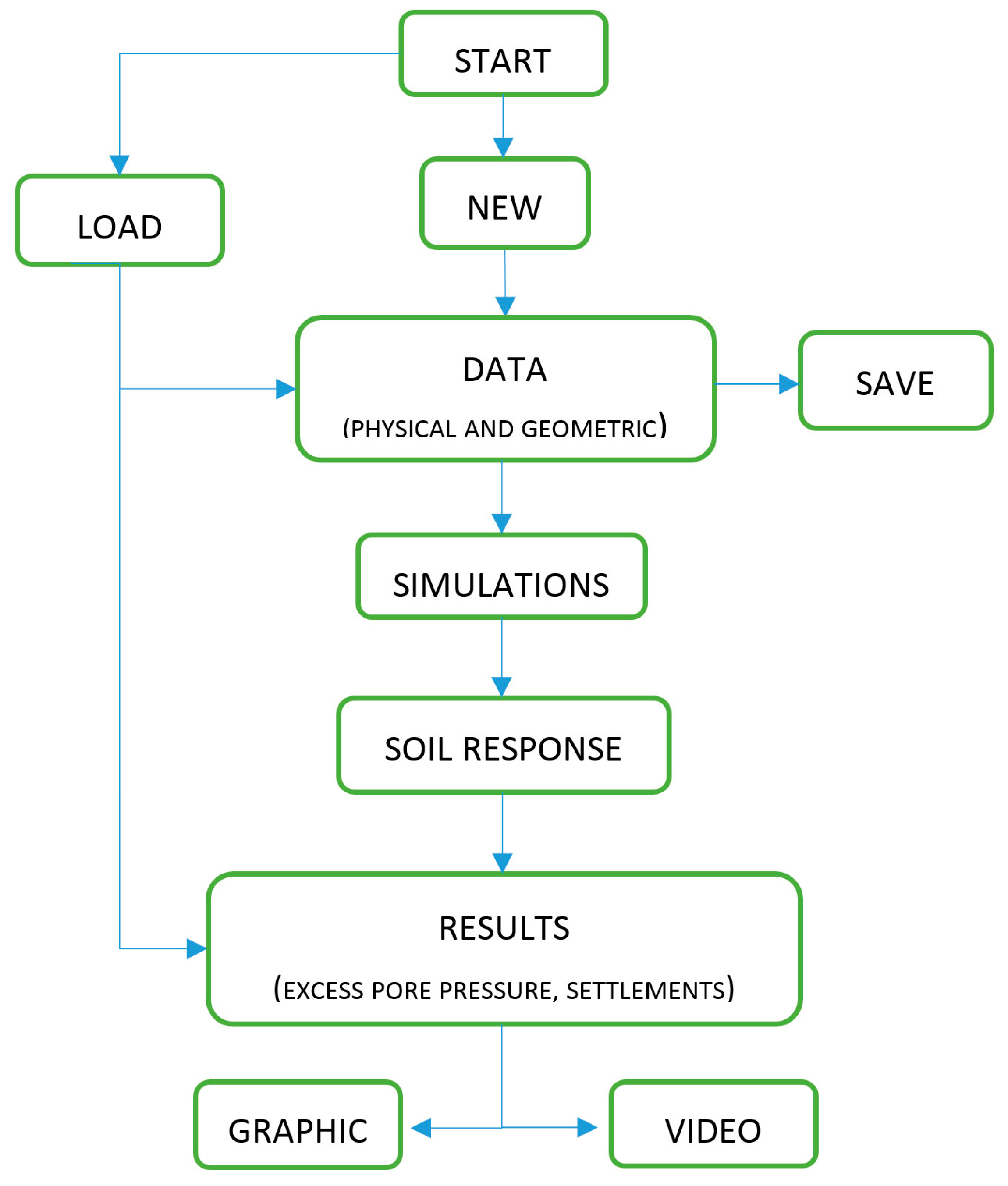
3. The Simulation Program
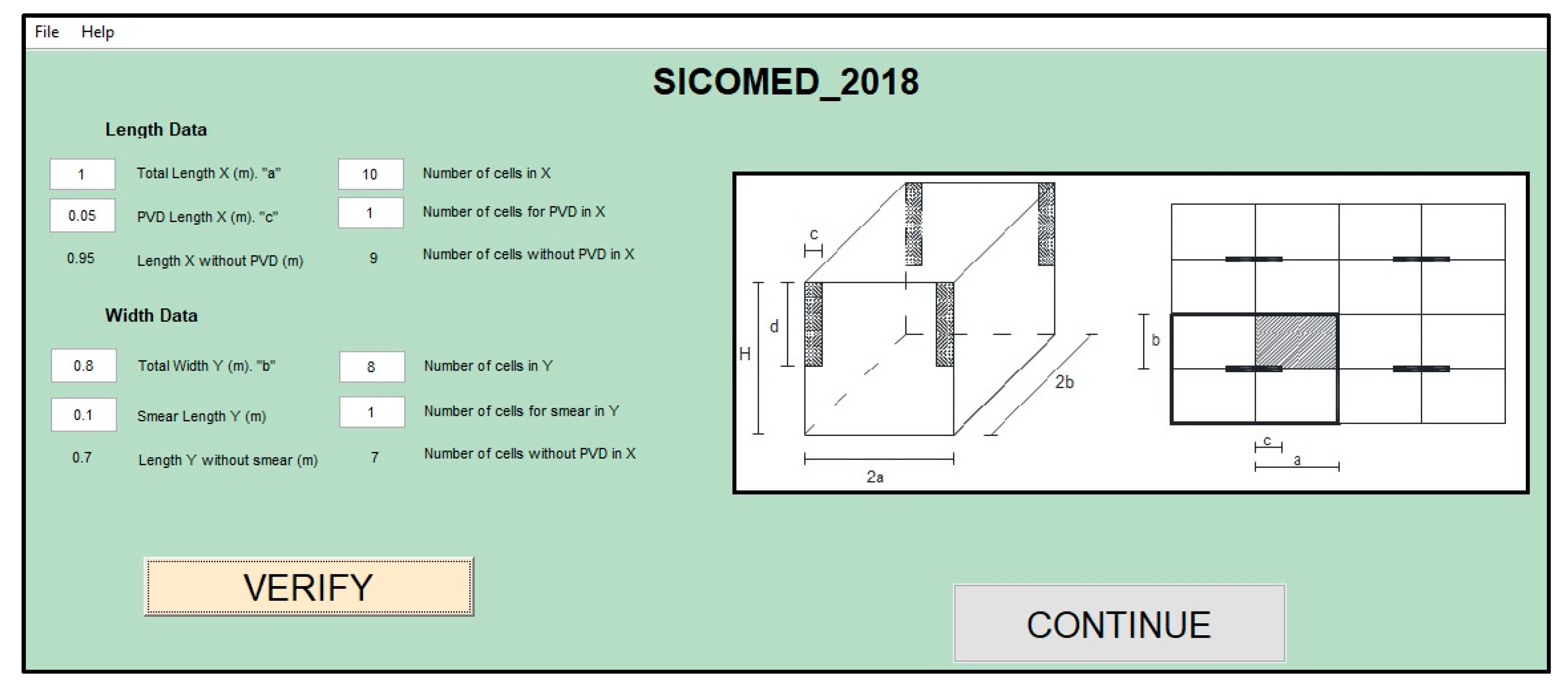
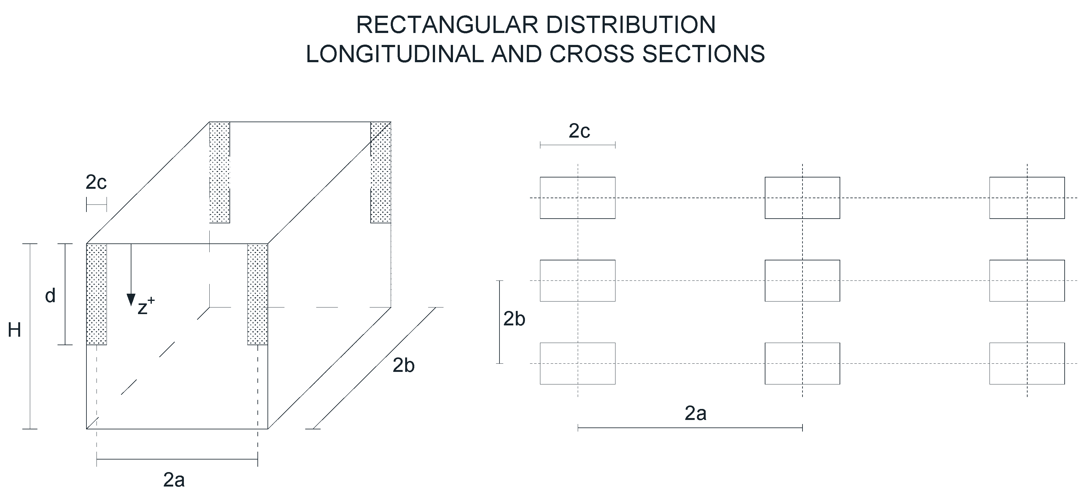
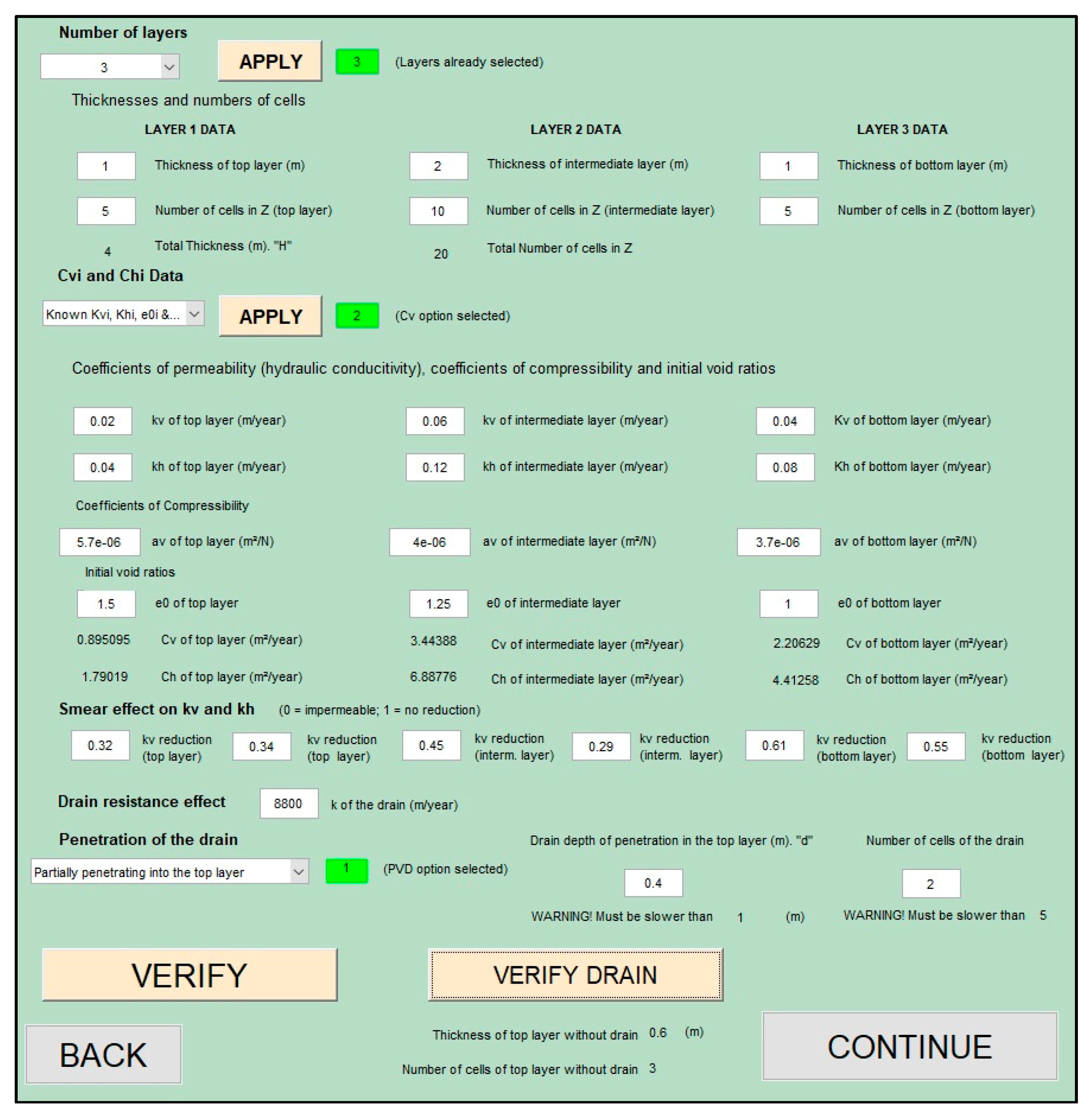
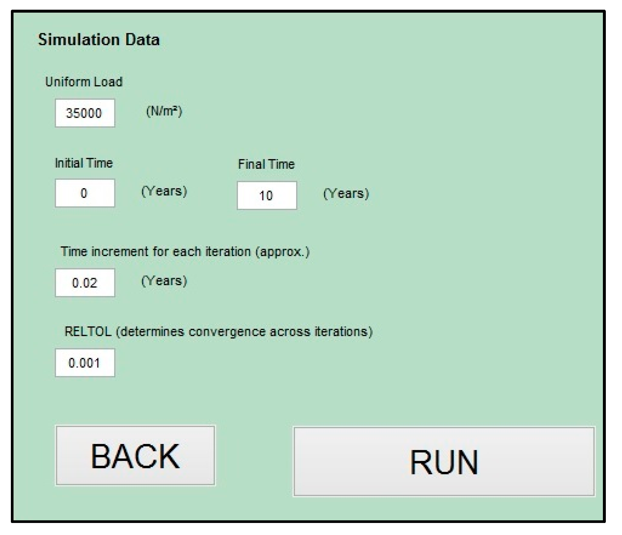
3.1. The Input Data and Network Design
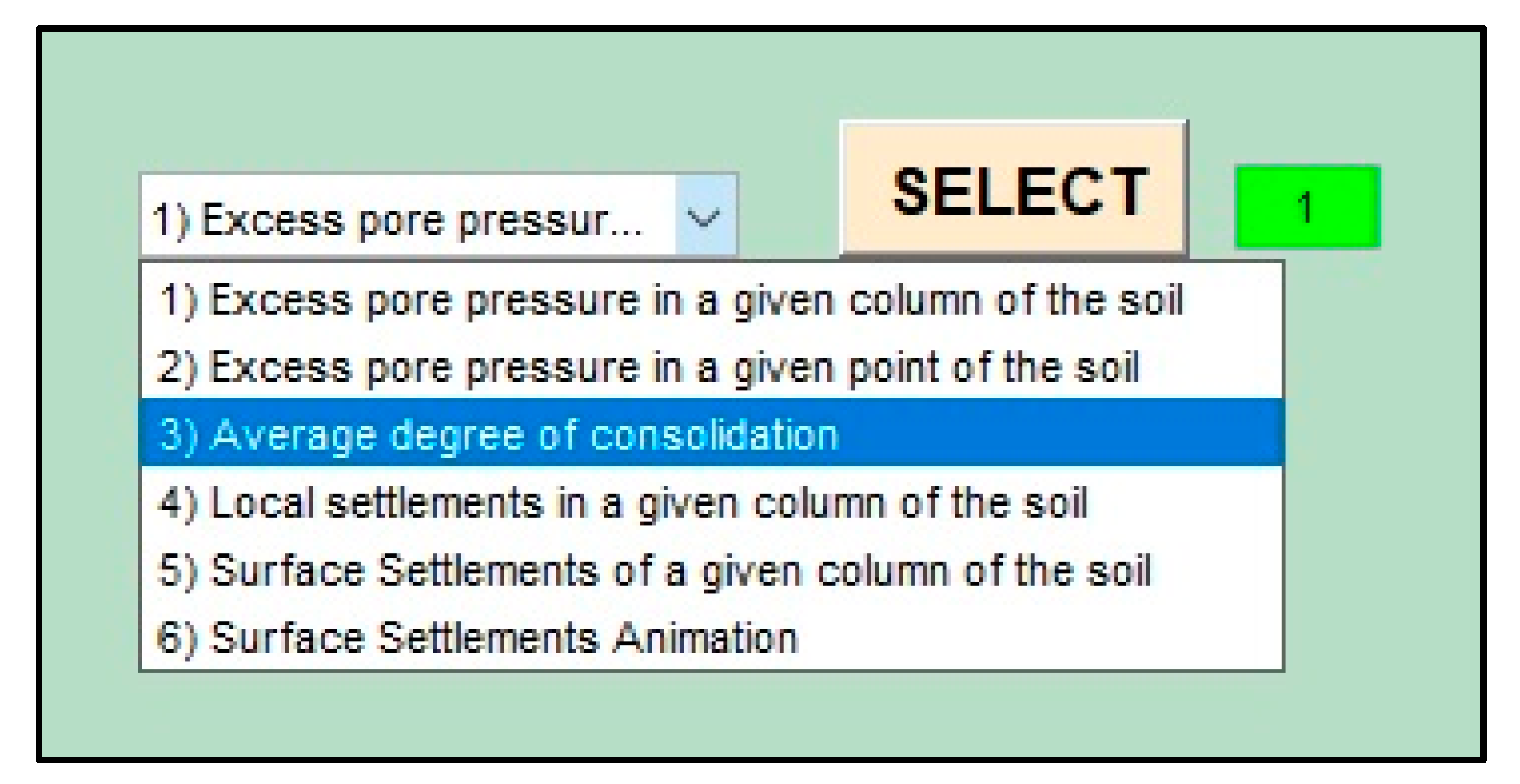
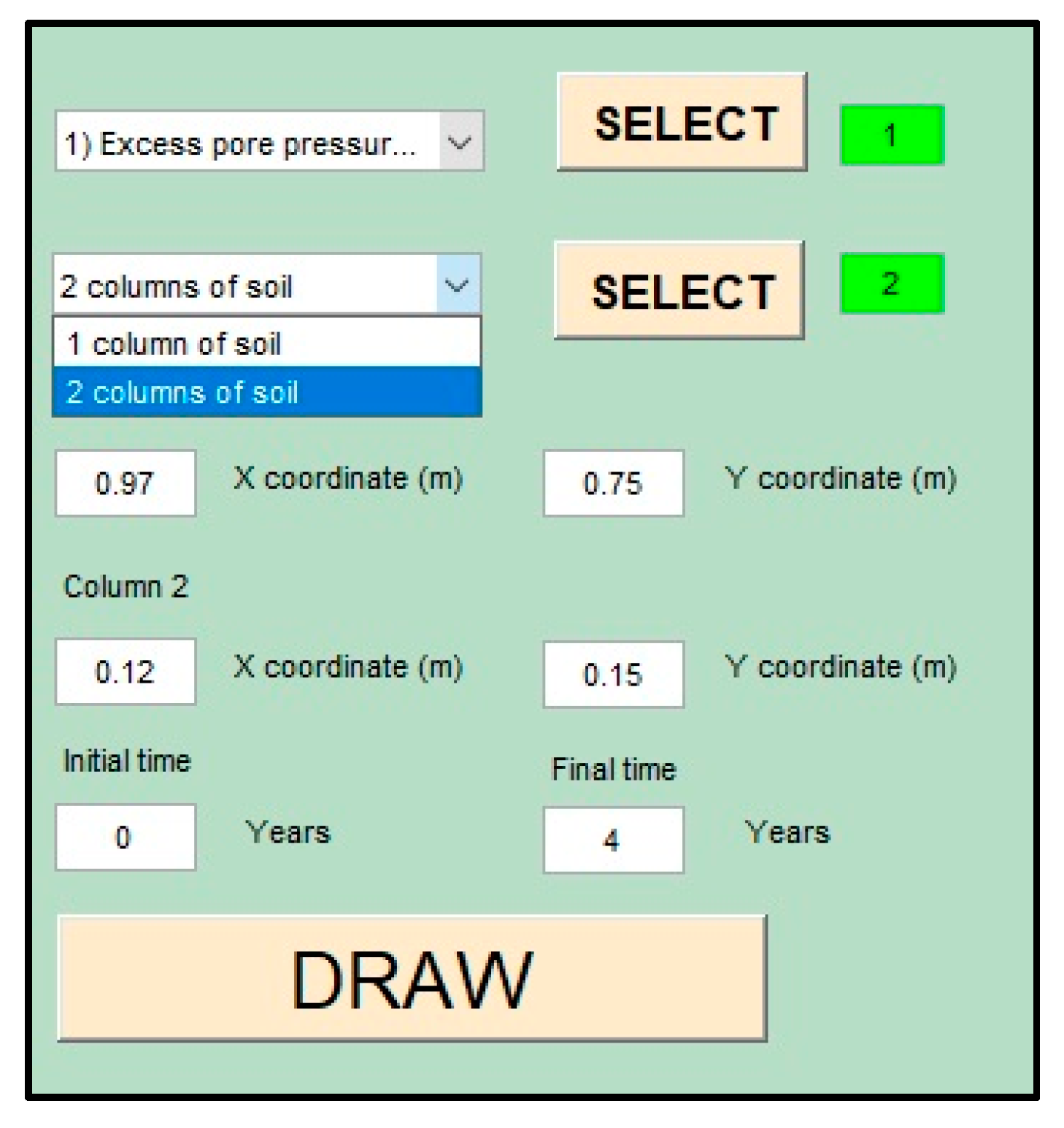
3.2. Simulation and Output Data
- Excess pore pressure in a given column of the soil
- Excess pore pressure in a given point of the soil
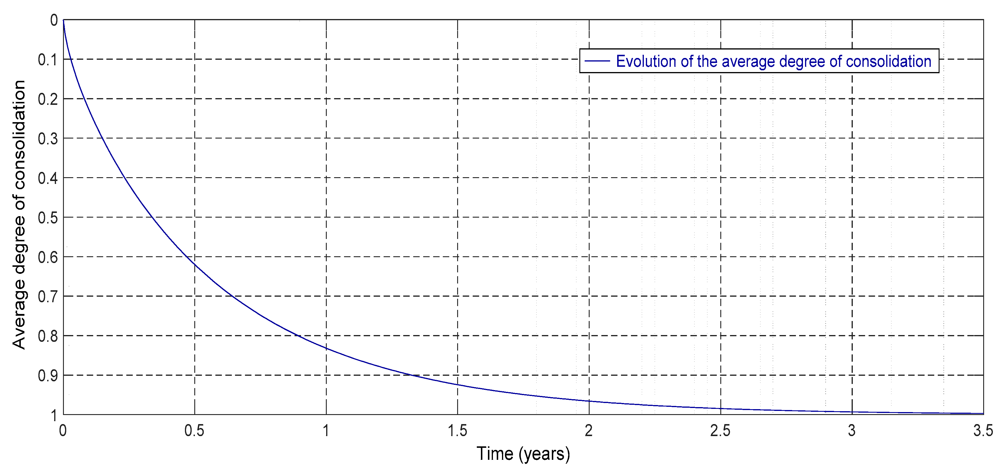
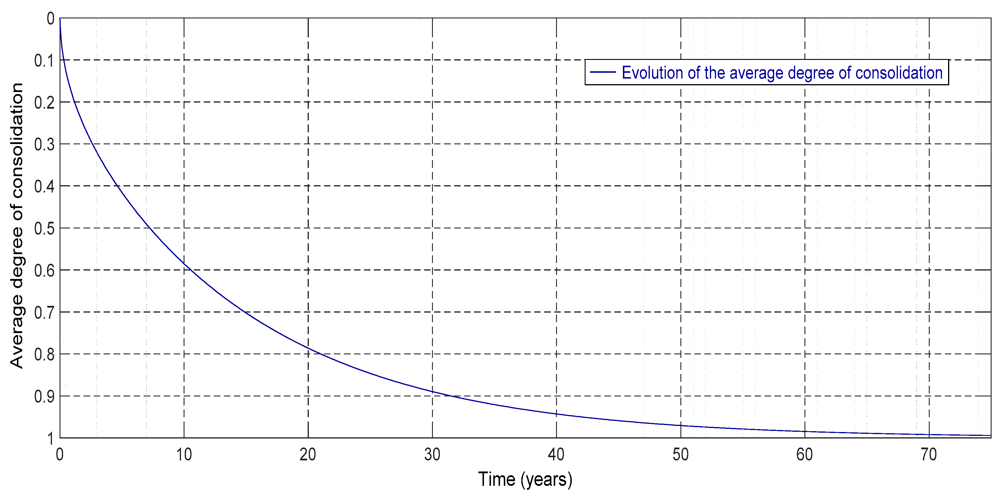
- Average degree of settlement
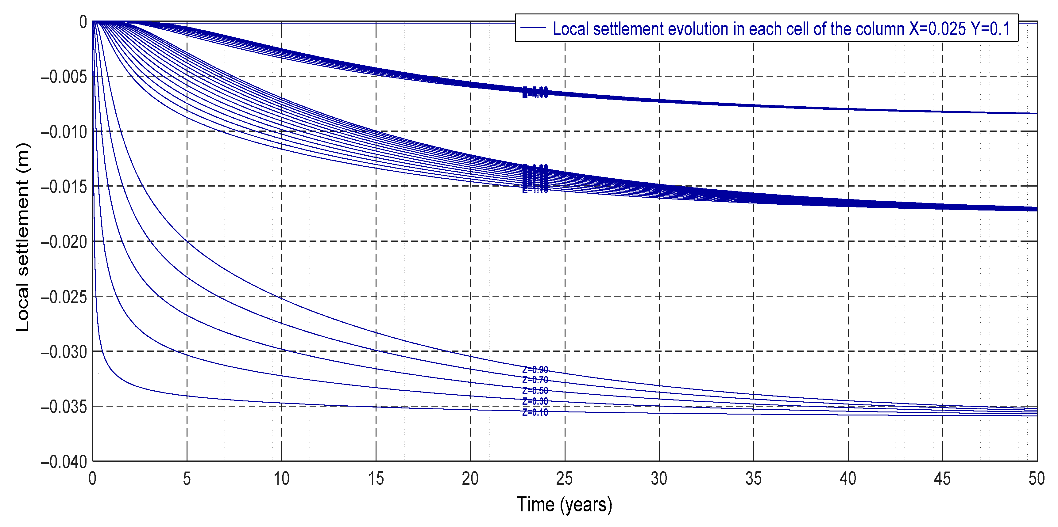
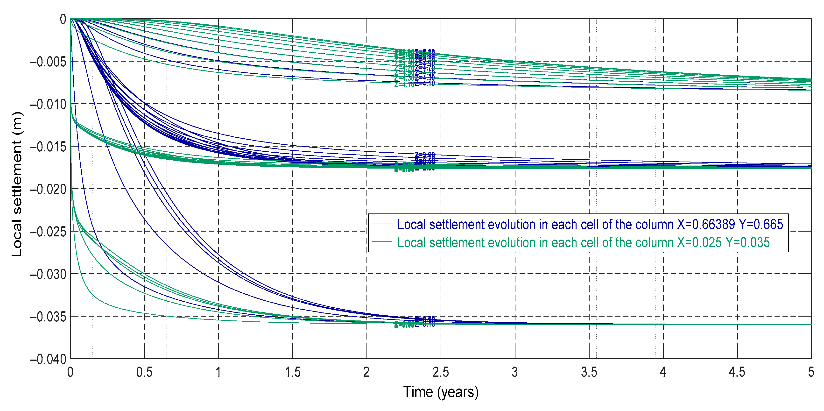
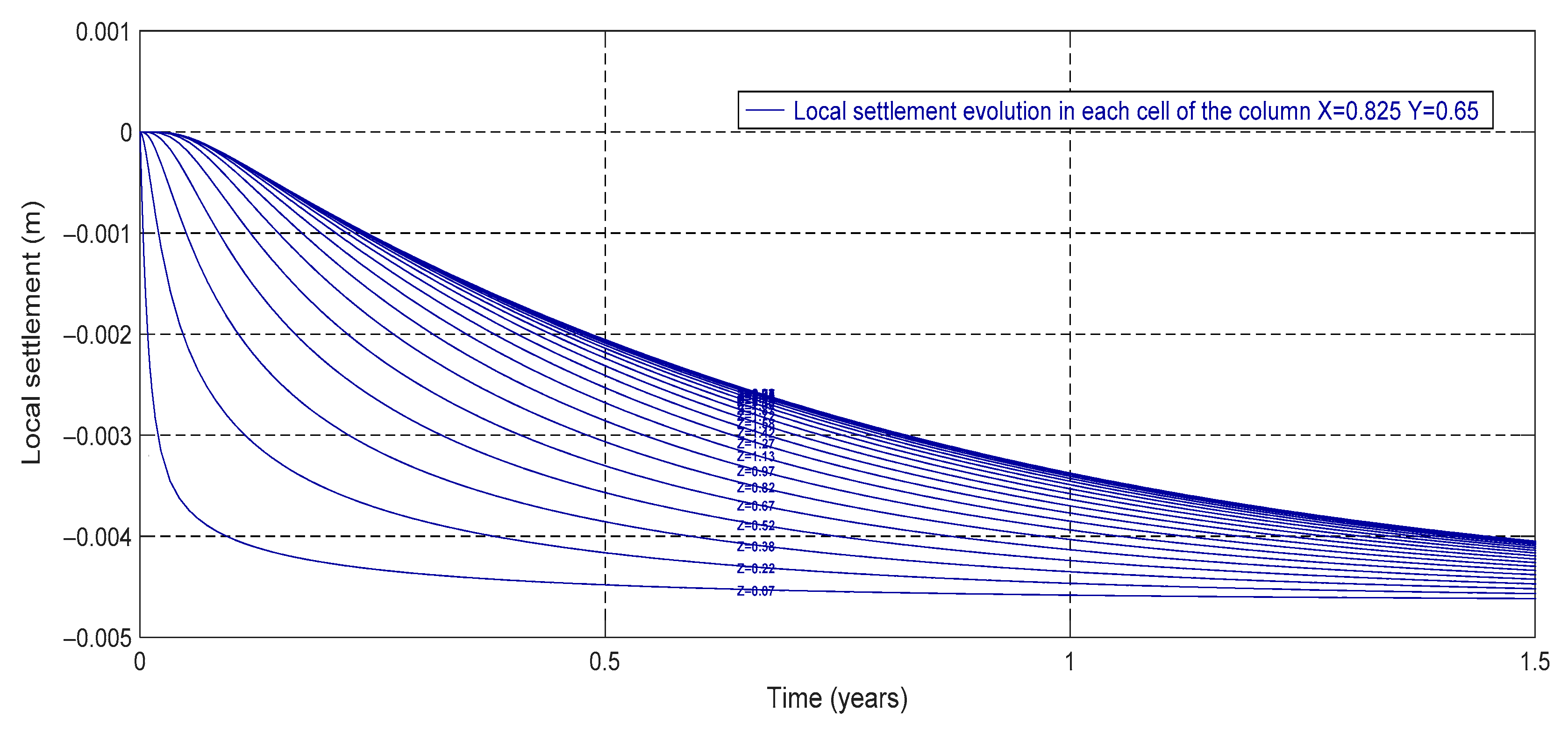
- Local settlements in a given column of the soil
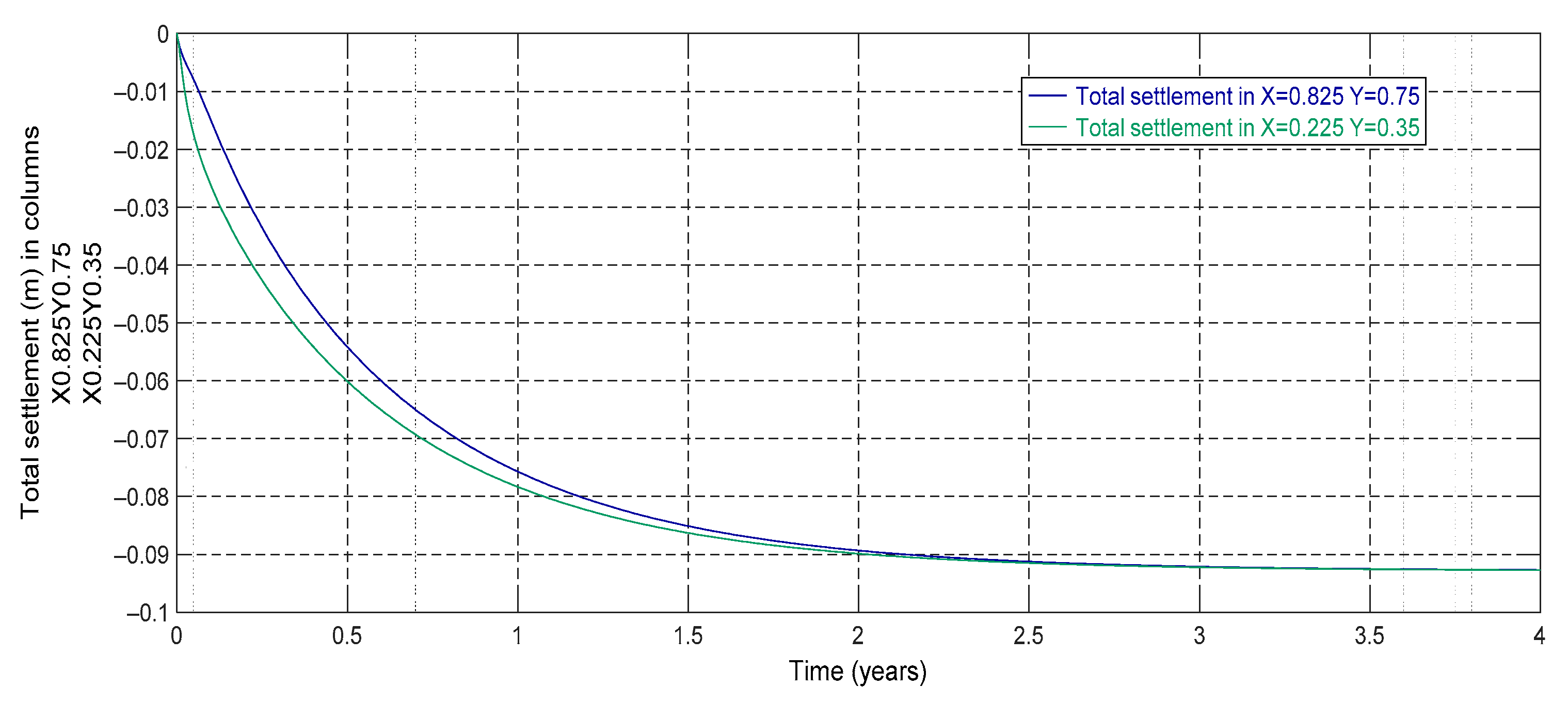
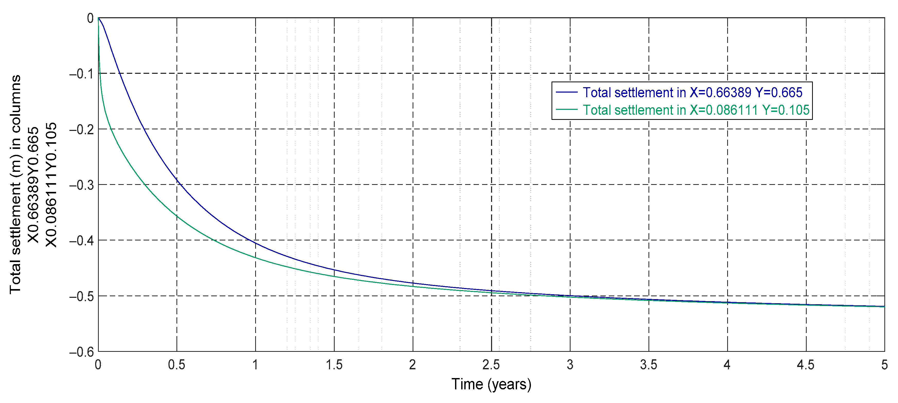
- Total settlement in a given point of the surface
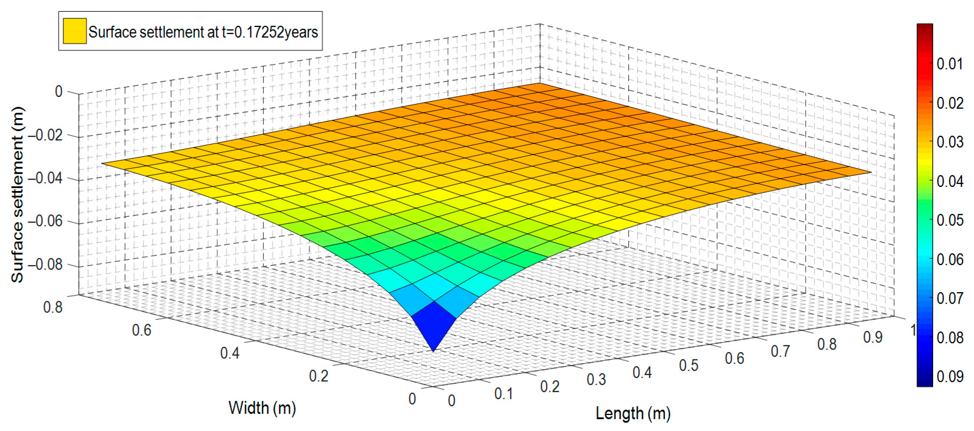
- Surface settlements animation.
4. Applications
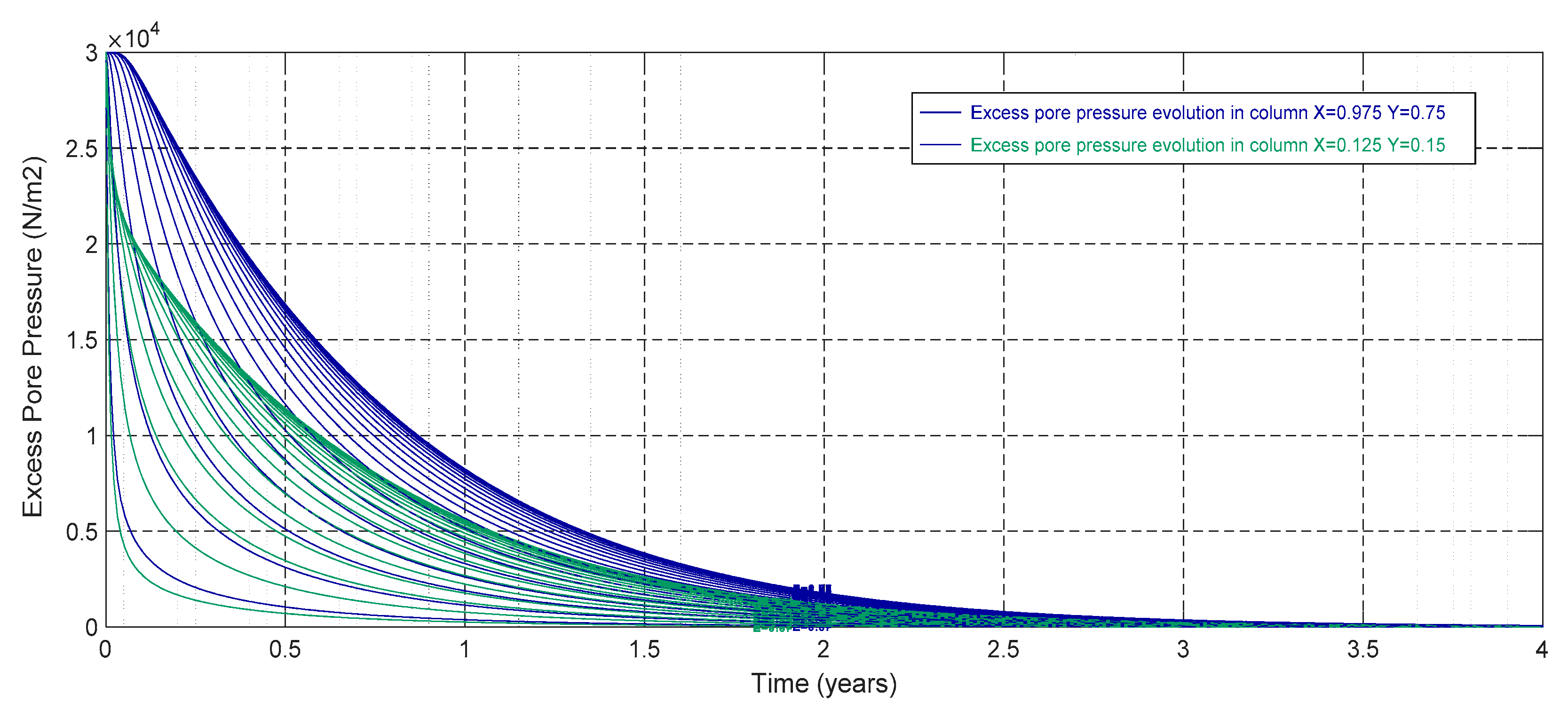
4.1. First Scenario: Consolidation of a One-Layer Soil with PVD
4.2. Second Scenario: Optimization of PVD Layout
4.3. Third Scenario: Influence of the Smear Zone and the Discharge Capacity Limitation of the PVD
5. Final Comments and Conclusions
Acknowledgments
Author Contributions
Conflicts of Interest
Nomenclature
| a | semi-separation between prefabricated vertical drains (m) |
| av | coefficient of compressibility (m2/N) |
| b | semi-separation between rows of prefabricated vertical drains (m) |
| c | Semi-width of prefabricated vertical drain (m) |
| C | capacity value of a capacitor (F) |
| Ci | capacitor connected between the central node of cell i and the common ground node |
| cv | coefficient of consolidation (m2/s) |
| cv,h | horizontal coefficient of consolidation (m2/s) |
| cv,x | horizontal coefficient of consolidation in x spatial direction (m2/s) |
| cv,y | horizontal coefficient of consolidation in y spatial direction (m2/s) |
| cv,z | vertical coefficient of consolidation (m2/s) |
| d | depth of penetration of prefabricated vertical drain (m) |
| e | void ratio (dimensionless) |
| eo | initial void ratio (dimensionless) |
| H | soil thickness or draining length of the water in vertical direction (m) |
| IC | current that flows through a capacitor (A) |
| IR | current that flows through a resistance (A) |
| JC | current flow associated with a capacitor (A) |
| JR | current flow associated with a resistance (A) |
| kd | hydraulic conductivity of the PVD (m/s) |
| kh | horizontal hydraulic conductivity of the undisturbed soil (m/s) |
| kh,s | horizontal hydraulic conductivity of the smear zone (m/s) |
| kv | vertical hydraulic conductivity of the undisturbed soil (m/s) |
| kv,s | vertical hydraulic conductivity of the smear zone (m/s) |
| n | normal direction to the boundary surface |
| Nx | number of cells in x direction |
| Ny | number of cells in y direction |
| Nz | number of cells in z direction |
| q | uniform load applied to the ground surface (N/m2) |
| qw | discharge capacity of the PVD for unit gradient of pressure (m3/s) |
| R | value of electrical resistance (Ω) |
| Rj | resistance connected between the central node of cell i and node j |
| t | time independent variable (s) |
| td | PVD thickness (m) |
| to | characteristic time of the consolidation process (s) |
| u | excess pore water pressure (N/m2) |
| U | local degree of settlement (dimensionless) |
| average degree of settlement (dimensionless) | |
| ui | excess pore pressure in node i (N/m2) |
| uo | initial excess pore pressure (N/m2) |
| VC | voltage between the terminals of a capacitor (V) |
| VR | voltage between the terminals of a resistance (V) |
| x | long horizontal spatial coordinate (m) |
| X | value of the spatial coordinate x (m) |
| y | wide horizontal spatial coordinate (m) |
| Y | value of the spatial coordinate y (m) |
| z | vertical spatial coordinate (m) |
| Z | value of the spatial coordinate z (m) |
| γw | specific weight of water (N/m3) |
| σ′f | final effective pressure (N/m2) |
| σ′o | initial effective pressure (N/m2) |
References
- Del Cerro Velázquez, F.; Gómez-Lopera, S.A.; Alhama, F. A powerful and versatile educational software to simulate transient heat transfer processes in simple fins. Comput. Appl. Eng. Educ. 2008, 16, 72–82. [Google Scholar] [CrossRef]
- Alhama, I.; Soto-Meca, A.; Alhama, F. Fatsim-A: An educational tool based on electrical analogy and the code PSpice to simulate fluid flow and solute transport processes. Comput. Appl. Eng. Educ. 2014, 22, 516–528. [Google Scholar]
- CODENS_13 [Software]. Coupled Ordinary Differential Equations by Network Simulation. © Universidad Politécnica de Cartagena, Sánchez, J.F., Alhama, I., Morales-Guerrero, J.L., Alhama, F. 2014. [Google Scholar]
- Manteca, I.A.; Alcaraz, M.; Trigueros, E.; Alhama, F. Dimensionless characterization of salt intrusion benchmark scenarios in anisotropic media. Appl. Math. Comput. 2014, 247, 1173–1182. [Google Scholar] [CrossRef]
- Conesa, M.; Pérez, J.S.; Alhama, I.; Alhama, F. On the nondimensionalization of coupled, nonlinear ordinary differential equations. Nonlinear Dyn. 2016, 84, 91–105. [Google Scholar] [CrossRef]
- SICOMED_2018 [Software]. Simulación de Consolidación Con Mechas Drenantes. © Universidad Politécnica de Cartagena, García-Ros, G., Alhama, I. 2018; (In registration phase). [Google Scholar]
- Karim, U.F. Simulation and video software development for soil consolidation testing. Adv. Eng. Softw. 2003, 34, 721–728. [Google Scholar] [CrossRef]
- Ngspice [Software]. Open Source Mixed Mode, Mixed Level Circuit Simulator (Based on Berkeley’s Spice3f5). Available online: http://ngspice.sourceforge.net/ (accessed on 31 January 2014).
- González-Fernández, C.F. Applications of the network simulation method to transport processes. In Network Simulation Method; Horno, J., Ed.; Research Signpost: Trivandrum, India, 2002. [Google Scholar]
- Alhama, F. Estudio de Respuestas Térmicas Transitorias en Procesos No Lineales de Transmisión de Calor Mediante el Método de Simulación Por Redes. Ph.D. Thesis, Universidad de Murcia, Murcia, Spain, 1999. [Google Scholar]
- Von Terzaghi, K. Die Berechnung der Durchassigkeitsziffer des Tones aus dem Verlauf der hydrodynamischen Spannungs. Erscheinungen. Sitzungsber. Akad. Wiss. Math. Naturwiss. Kl. Abt. 2A 1923, 132, 105–124. [Google Scholar]
- Taylor, D.W. Fundamentals of Soil Mechanics; Wiley: New York, NY, USA, 1948. [Google Scholar]
- Berry, P.L.; Reid, D. An Introduction to Soil Mechanics; McGraw-Hill: London, UK, 1987. [Google Scholar]
- Davis, E.H.; Raymond, G.P. A non-linear theory of consolidation. Géotechnique 1965, 15, 161–173. [Google Scholar] [CrossRef]
- Manteca, I.A.; García-Ros, G.; López, F.A. Universal solution for the characteristic time and the degree of settlement in nonlinear soil consolidation scenarios. A deduction based on nondimensionalization. Commun. Nonlinear Sci. Numer. Simul. 2018, 57, 186–201. [Google Scholar] [CrossRef]
- Hansbo, S.; Jamiolkowski, M.; Kok, L. Consolidation by vertical drains. Géotechnique 1981, 31, 45–66. [Google Scholar] [CrossRef]
- Indraratna, B.; Redana, I.W. Numerical modeling of vertical drains with smear and well resistance installed in soft clay. Can. Geotech. J. 2000, 37, 132–145. [Google Scholar] [CrossRef]
- Conte, E.; Troncone, A. Radial consolidation with vertical drains and general time-dependent loading. Can. Geotech. J. 2009, 46, 25–36. [Google Scholar] [CrossRef]
- Castro, E.; García-Hernández, M.T.; Gallego, A. Transversal waves in beams via the network simulation method. J. Sound Vib. 2005, 283, 997–1013. [Google Scholar] [CrossRef]
- Morales-Guerrero, J.L.; Moreno-Nicolás, J.A.; Alhama, F. Application of the network method to simulate elastostatic problems defined by potential functions. Applications to axisymmetrical hollow bodies. Int. J. Comput. Math. 2012, 89, 1781–1793. [Google Scholar] [CrossRef]
- Sánchez, J.F.; Alhama, F.; Moreno, J.A. An efficient and reliable model based on network method to simulate CO2 corrosion with protective iron carbonate films. Comput. Chem. Eng. 2012, 39, 57–64. [Google Scholar] [CrossRef]
- Bég, O.A.; Takhar, H.S.; Zueco, J.; Sajid, A.; Bhargava, R. Transient Couette flow in a rotating non-Darcian porous medium parallel plate configuration network simulation method solutions. Acta Mech. 2008, 200, 129–144. [Google Scholar] [CrossRef]
- Marín, F.; Alhama, F.; Moreno, J.A. Modelling of stick-slip behavior with different hypotheses on friction forces. Int. J. Eng. Sci. 2012, 60, 13–24. [Google Scholar] [CrossRef]
- Cánovas, M.; Alhama, I.; Trigueros, E.; Alhama, F. Numerical simulation of Nusselt-Rayleigh correlation in Bénard cells. A solution based on the network simulation method. Int. J. Numer. Methods Heat Fluid Flow 2015, 25, 986–997. [Google Scholar] [CrossRef]
- Li, Y.; Chen, Y.F.; Zhang, G.J.; Liu, Y.; Zhou, C.B. A numerical procedure for modeling the seepage field of water-sealed underground oil and gas storage caverns. Tunn. Undergr. Space Technol. 2017, 66, 56–63. [Google Scholar] [CrossRef]
- Taormina, R.; Chau, K.W.; Sivakumar, B. Neural network river forecasting through baseflow separation and binary-coded swarm optimization. J. Hydrol. 2015, 529, 1788–1797. [Google Scholar] [CrossRef]
- Chen, X.Y.; Chau, K.W. A Hybrid Double Feedforward Neural Network for Suspended Sediment Load Estimation. Water Resour. Manag. 2016, 30, 2179–2194. [Google Scholar] [CrossRef]
- Olyaie, E.; Banejad, H.; Chau, K.W.; Melesse, A.M. A comparison of various artificial intelligence approaches performance for estimating suspended sediment load of river systems: A case study in United States. Environ. Monit. Assess. 2015, 187. [Google Scholar] [CrossRef] [PubMed]
- Chau, K.W. Use of Meta-Heuristic Techniques in Rainfall-Runoff Modelling. Water 2017, 9, 186. [Google Scholar] [CrossRef]
- González, L.M.; Sánchez, J.F.; Barberá, M. Comparación de los softwares utlizados para el cálculo de inmisión en procesos de incineración. Gac. Sanit. 2017, 31, 73. [Google Scholar]
- Sánchez, J.F.; González, L.M.; Barberá, M. Análisis de la altura de la chimenea en procesos de incineración mediante análisis dimensional. Gac. Sanit. 2017, 31, 330. [Google Scholar]
- García-Ros, G.; Alhama, I. SICOMED_3D: Simulación y Diseño de Problemas de Consolidación de Suelos Con Mechas Drenantes; Universidad Politécnica, CRAI Biblioteca: Cartagena, Spain, 2017. [Google Scholar]
- García-Ros, G. Caracterización Adimensional y Simulación Numérica de Procesos Lineales y No Lineales de Consolidación de Suelos. Ph.D. Thesis, Universidad Politécnica de Cartagena, Cartagena, Spain, 2016. [Google Scholar]
- Barron, R.A. Consolidation of fine grained soils by drain wells. Trans. ASCE 1948, 113, 718–742. [Google Scholar]


| Thickness (H) | 3 m |
| Separation between PVDs (2a) | 2 m |
| Separation between rows of PVDs (2b) | 1.6 m |
| PVD width (2c) | 0.1 m |
| Depth of penetration of PVD (d) | 3 m |
| Applied load (q) | 30 kN/m2 |
| Initial void ratio (eo) | 1.23 |
| Compressibility coefficient (av) | 0.0023 m2/kN |
| Vertical hydraulic conductivity (kv) | 0.0095 m/year |
| Horizontal hydraulic conductivity (kh) | 0.0259 m/year |
| Vertical consolidation coefficient (cv,z) | 0.94 m2/year |
| Horizontal consolidation coefficient (cv,h) | 2.56 m2/year |
| Soil Property | S1 (Upper Stratum) | S2 (Intermediate Stratum) | S3 (Lower Stratum) | |
|---|---|---|---|---|
| Thickness (m) | H | 1 | 3 | 2 |
| Initial void ratio | eo | 1.5 | 0.9 | 0.7 |
| Compressibility coefficient (m2/kN) | av | 0.0075 | 0.0028 | 0.00125 |
| Vertical hydraulic conductivity (m/year) | kv | 0.007 | 0.015 | 0.006 |
| Horizontal hydraulic conductivity (m/year) | kh | 0.022 | 0.04 | 0.01 |
| Vertical consolidation coefficient (m2/year) | cv,z | 0.24 | 1.04 | 0.83 |
| Horizontal consolidation coefficient (m2/year) | cv,h | 0.75 | 2.77 | 1.39 |
| Depth of PVD (m) | to (Years) |
|---|---|
| Without drain | 32 |
| 1 | 27 |
| 4 | 4.5 |
| 6 | 3 |
| Depth of PVD (m) | to (Years) |
|---|---|
| Without drain | 32 |
| 1 (a = b = 1 m) | 27 |
| 4 (a = b = 1 m) | 4.5 |
| 6 (a = b = 1 m) | 3 |
| 6 (a = b = 0.9 m) | 2.4 |
| 6 (a = b = 0.8 m) | 1.9 |
| 4 (a = b = 0.8 m) | 2.5 |
| 4 (a = b = 0.7 m) | 2.0 |
| 4 (a = b = 0.65 m) | 1.8 |
| Parameter/Soil Property | Value | Units |
|---|---|---|
| H (draining length) | 15 | m |
| 2a (separation between PVDs) | 0.785 | m |
| 2b (separation between rows PVDs) | 0.739 | m |
| 2c (PVD width) | 0.0924 | m |
| td (PVD thickness) | 0.005 | m |
| PVD equivalent diameter | 0.0620 | m |
| Smear length (normal to the PVD plain) | 0.0693 | m |
| kh (horizontal hydraulic conductivity of the undisturbed soil) | 0.03 | m/year |
| kh,s (horizontal hydraulic conductivity of the smear zone) | 0.01 | m/year |
| kv (vertical hydraulic conductivity of the undisturbed soil) | 0.009 | m/year |
| kv,s (vertical hydraulic conductivity of the smear zone) | 0.003 | m/year |
| cv,h (horizontal consolidation coefficient) | 0.5 | m2/year |
| cv,z (vertical consolidation coefficient) | 0.15 | m2/year |
| Grid size (Nx, Ny, Nz) | 17 × 16 × 15 | |
| Drain hydraulic conductivity for qw = 20 m3/year | 43,290 | m/year |
| Drain hydraulic conductivity for qw = 10 m3/year | 21,645 | m/year |
| Drain hydraulic conductivity for qw = 5 m3/year | 10,822.5 | m/year |
| Case | t = 0.5 Years | t = 1 Years | t = 2 Years | ||||||
|---|---|---|---|---|---|---|---|---|---|
| Barron | Hansbo | SICOMED (% Error) | Barron | Hansbo | SICOMED (% Error) | Barron | Hansbo | SICOMED (% Error) | |
| Case 1 No smear, limited discharge capacity | 66.3% | - | 68.1% (2.71%) | 89.2% | - | 89.6% (0.45%) | 98.6% | - | 98.9% (0.30%) |
| Case 2 Smear zone, qw = 20 m3/year | - | 46.0% | 44.5% (−3.26%) | - | 69.8% | 68.8% (−1.43%) | - | 90.5% | 90.2% (−0.33%) |
| Case 3 Smear zone, qw = 10 m3/year | - | 41.8% | 39.1% (−6.46%) | - | 63.3% | 62.5% (−1.26%) | - | 86.0% | 85.5% (−0.58%) |
| Case 4 Smear zone, qw = 5 m3/year | - | 34.5% | 30.5% (−11.6%) | - | 53.9% | 50.9% (−5.57%) | - | 77.9% | 74.8% (−3.98%) |
© 2018 by the authors. Licensee MDPI, Basel, Switzerland. This article is an open access article distributed under the terms and conditions of the Creative Commons Attribution (CC BY) license (http://creativecommons.org/licenses/by/4.0/).
Share and Cite
García-Ros, G.; Alhama, I.; Cánovas, M. Powerful Software to Simulate Soil Consolidation Problems with Prefabricated Vertical Drains. Water 2018, 10, 242. https://doi.org/10.3390/w10030242
García-Ros G, Alhama I, Cánovas M. Powerful Software to Simulate Soil Consolidation Problems with Prefabricated Vertical Drains. Water. 2018; 10(3):242. https://doi.org/10.3390/w10030242
Chicago/Turabian StyleGarcía-Ros, Gonzalo, Iván Alhama, and Manuel Cánovas. 2018. "Powerful Software to Simulate Soil Consolidation Problems with Prefabricated Vertical Drains" Water 10, no. 3: 242. https://doi.org/10.3390/w10030242
APA StyleGarcía-Ros, G., Alhama, I., & Cánovas, M. (2018). Powerful Software to Simulate Soil Consolidation Problems with Prefabricated Vertical Drains. Water, 10(3), 242. https://doi.org/10.3390/w10030242