Sensitivity Analysis for the Inverted Siphon in a Long Distance Water Transfer Project: An Integrated System Modeling Perspective

1
School of Hydraulic Engineering, Dalian University of Technology, Dalian 116024, China
2
Faculty of Management and Economics, Dalian University of Technology, Dalian 116024, China
*
Author to whom correspondence should be addressed.
Water 2018, 10(3), 292; https://doi.org/10.3390/w10030292
Submission received: 3 February 2018
/
Revised: 5 March 2018
/
Accepted: 6 March 2018
/
Published: 8 March 2018
(This article belongs to the Special Issue Adaptive Catchment Management and Reservoir Operation)
Abstract
:Long distance water diversion projects are developed to alleviate the conflicts between supply and demand of water resources across different watersheds. However, the significant scale water diversion projects bring new challenges for the water supply security. This paper presents the flood risk of inverted siphon structure which is used for crossing transversally in the water diversion project through sensitivity analysis. Soboĺ and regionalized sensitivity analysis are used to investigate the sensitive parameters of the integrated model and the sensitive range of the parameters, respectively. The integrated system model consists of the hydrologic model, the sediment transport model and the siphon hydraulic model to determine the flood overtopping duration and volume, which are used to quantify flood risk in this study. The flood overtopping duration and volume indicators are used to quantify flood risk in the sensitivity analysis. The South to North Water Diversion Project in China is used as a case study. The results show the mean rainfall and roughness coefficient of the pipe are the most sensitive parameters in the integrated models, while the sensitive range of these two parameters are distinct. The sensitivity analysis of the inverted siphon provides an insight into the significant contributions to the flood risk. The analysis can provide the guidance for the system operation security.
1. Introduction
Due to urbanization and the uneven distribution of water resources in time and space, long-distance water transfer projects are constructed to alleviate the shortage of water resource and meet the increasing demands [1,2,3]. Water transfer projects often involve huge capital investment and pose complex security problems [4,5,6]. For example, canals usually cross hundreds of kilometers of complicated terrain, which leads to water quality deterioration, temperature variation, and long operation response period. Moreover, critical hydraulic structures are essential for ensuring the operation security of the projects, e.g., gate/valve, pump station, and intersection structures. Here, we focus on the inverted siphon structure, which is linked to the river to drain water by gravity that is collected from a relatively small hydrographic basin, so that the river can cross transversally a large artificial open channel carrying fresh water for supply.
Inverted siphon structures are prone to be impacted by the hydraulic transient process and structure stability. The potential failures of inverted siphons can be divided into two categories: (1) structure failure; and (2) operation failure. Structure failure indicates the structure identity is destroyed or collapsed due to structure aging and external forces. Operation failure refers to the flows exceeding the design standard of inverted siphon. That is because the designed flood and flood design standard that are used to guide the structure design are subject to the hydrologic parameter uncertainties (e.g., rainfall, soil moisture, and land use) and the hydraulic uncertainties (e.g., sediment deposition). The extra upstream flow of inverted siphon is retained at the entry and a large flood can potentially enter the canal and contaminate the quality of source water in the canal. Therefore, there is a need to investigate which uncertain parameters (e.g., rainfall, sediments, and pipe roughness coefficient) can significantly contribute to the flooding incidents. This paper utilizes an inverted siphon structure that passes underneath a long distance transfer project to illustrate the flood overtopping risk. The sensitivity analysis with respect to inverted siphons is of vital importance to guarantee the safe operation of the long-distance transfer project.
Sensitivity Analysis (SA) has gathered plenty of attention for describing the sensitivity of parameters in terms of the contributions to the model output [7]. Global SA method, in contrast to local SA, is capable of accounting for the whole range of input parameter variation to avoid the subjective judgment and case-specific characteristics on the parameter range. The global SA can deal with the non-linear and non-monotonic models [8,9,10]. Another type of SA is regression-related, e.g., Multivariate Adaptive Regression Splines (MARS), Gaussian Process (GP) and Radial Basis Function [11]. They use linear or non-linear models to refit the original model and investigate which parameters can give the relative large reduction in goodness-of-fit. The large reduction represents the sensitive parameters [12]. The regression sensitivity methods have the advantage of less computational effort. Moreover, Soboĺ SA [13] is typically a variance based method. It decomposes the response variances for the specific order SA indices. The Soboĺ SA method can calculate the interactions among input parameters, but it should be noted that the higher order Soboĺ analysis could significantly increase the computational burden with the increase in the input number [14,15,16]. Regional Sensitivity Analysis (RSA) was developed by Spear and Hornberger [17] and improved by Beven and Binley [18], which is also a global SA method. RSA elaborates the sensitivity variation over the full range for a given parameter. The cumulative possibility of behavioral sets is investigated in the RSA to reflect the parameter interaction implicitly. Both Soboĺ and RSA methods are employed in this paper to ascertain the sensitive parameters in the inverted siphon flooding model [19].
This paper aims to address the sensitivities of any value over the domain of the parameters and further identifies the sensitive parameters in the inverted siphon models. The sensitive parameter screening and sensitive range identification of the parameters are implemented by Soboĺ SA and RSA methods, respectively. The upstream runoff of the siphon is simulated by a local hydrologic model, and the sediment transportation and pipe transmission model are used to calculate the inverted siphon flows. The evaluation indexes (flood overtopping duration and volume) are set up to demonstrate the flood risk of the inverted siphon. The sensitivity analysis results are demonstrated based on an inverted siphon structure across the South to North Water Diversion project.
2. Methods
The sensitivity analysis methods including Soboĺ SA and RSA method are introduced to evaluate the sensitivity of parameters in the integrated system modeling. The integrated system model is set up by integrating hydrologic model, sediment transport model and inverted siphon hydraulic model. Then, the two evaluation indicators, i.e., flood overtopping duration and volume, are used to quantify flood risk.
2.1. Sensitivity Analysis Methods
2.1.1. General
Two global sensitivity analysis methods are employed in this paper for investigating parameter sensitivity in consideration with the interaction of variables and the sensitivity variation over the range of the variables. The model can be represented by a numerical function,
where is the model output (or objective function) and is the variable set, .
2.1.2. Soboĺ Sensitivity Analysis
The Soboĺ sensitivity analysis [13,20] is a variance-based method, which uses variance decomposition to derive a variance ratio. It can provide a quantitative description of how individual variables and their interactions affect model performance [21]. An individual model parameter and its interaction with other parameters contribute to the total output variance, and the function is shown as follows:
where is the total variance of the output variable ; is given by the variance of the conditional expectation and to the interactions among parameters. To assess the role of each variable or interaction between variables, sensitivity measures are needed. The chosen measures are known as Soboĺ indices. The indices represent the bias in the variance of the output, which is attributed to a variable or a combination of variables. The first-order index is
and the second-order index is
The total order sensitivity index of a single parameter and this parameter’s interaction with other parameters, at least one index being from 1 to , is as follows:
The first-order sensitivity index only represents the individual contribution of variable to the model output. The second-order index indicates the interaction effect of two variables on the model output. The total-order index measures the main effect of parameter xi and its interactions with all the other variables. The Soboĺ indices are obtained by a sampling process, e.g., Latin Hypercube.
2.1.3. Regionalized Sensitivity Analysis
Regionalized sensitivity analysis (RSA) is proposed by Spear and Hornberger [17] and further extended by Beven and Binley [18]. RSA method is broadly applied in hydrology and environmental system analysis [19,22,23]. The approach is based on the Monte Carlo simulation considering possible combination of uncertain parameters with the given possibility density function. The parameters sampling process can cover the whole distribution range, so RSA also belongs to the global sensitivity analysis category. The sampled parameter sets are divided into behavioral or non-behavioral. If the computational result of a parameter set (objective function evaluations) satisfies the prescribed condition (e.g., less than a threshold), the parameter set is behavioral, vice versa.
RSA results are expressed by the cumulative distribution. The difference between the behavioral and non-behavioral cumulative distributions is larger, and then the parameter is more sensitive. Kolmogorov-Smirnoff (K-S) test is used to show the maximum vertical distance between the behavioral and non-behavioral cumulative distributions. The K-S test function is given as
where are the behavioral and non-behavioral cumulative distributions, respectively.
2.2. Definition of Evaluation Indicators
If the water level at the inlet of the inverted siphon exceeds the embankment crest elevation of the canal (denoted by Zs), then the flooding water will flow into the main trunk canal, i.e., flood overtopping happens. The event occurrence represents the inverted siphon hydraulic failure. This failure will bring the risks that are the embankment erosion and the water quality pollution for example. The longer duration of flood overtopping leads to more severe hazards and exaggerating the impacted extent on the canal. Therefore, we adopt the flood overtopping duration and flood overtopping volume as the indicators to evaluate the risk of flood overtopping for the inverted siphon.
It is assumed that the water level at the water inlet of the inverted siphon can rise, even if it exceeds the crest elevation of the canal Zs (i.e., there is a virtual water pond with unlimited crest elevation). The time periods, when water level exceeds Zs, are defined as the duration of flood overtopping. The flood overtopping volume can be calculated by the difference of maximum flood volume at the inlet and the volume that corresponds to the embankment crest elevation. The volumes are calculated by the water level–storage relationship at the inlet of the inverted siphon.
2.3. System Modeling
2.3.1. General
The input parameters that need to be tested in the sensitivity analysis are assigned by a set of random values (). The hydrologic model simulates the inflow of the inverted siphon in a given watershed. Sediment transport model is introduced to model the sand movement and deposition. Siphon hydraulic model is used to calculate the flow of the siphon. These three models are integrated and convey the parameter values, as shown in Figure 1. The outputs of the models are runoff, flow, sand content and water level. Two evaluation indexes are formulated by these outputs. The whole flow chart of the methodology is shown in Figure 1.
2.3.2. Hydrologic Model
Due to the lack of monitoring data in small watersheds, the Inferential Formula Method is often used to determine the design floods [24]. This study uses the Inferential Formula Method specified in China’s design flood regulations and proposed by Chen [25]. The flood is derived from design rainfall in the assumption that rainfall frequency is the same with flood frequency. The flood calculation includes the following steps:
(1) The maximum rainfall
The maximum rainfall during t h (for small watersheds, t is set to be 24 h) can be calculated by
where represents the amount of rainfall with the frequency for h (mm); is the average of maximum rainfall for h (mm); is a frequency factor; and is the coefficient of variation of maximum rainfall for h.
(2) The peak discharge
Rational method [26] is one of the earliest methods to estimate the peak discharge according to the rainfall data. When the runoff generation time (denoted by tc) is larger than the runoff concentration time (denoted by ), i.e., tc ≥ τ, the peak discharge is consisted of the runoff from the whole watershed. Assuming the runoff intensity is evenly distributed both in spatial and temporal, and the concentration is irrespective to the channels and slops, then the peak discharge is calculated by
in which, F denotes the area of the watershed (km2) and is the runoff concentration time (h), calculated based on the terrain characteristic for the given area,
is the amount of runoff generation during hours (mm), given by the following equation under the assumption of excess infiltration, that is, there is runoff generation only when the rainfall intensity is larger than the infiltration rate.
In Equations (9) and (10), γ is the rainfall diminishing exponent; is the average infiltration rate during h (mm/h); is the longest length from the outlet of main river to watershed outline (km); is the average slope for the longest path of runoff; is the runoff parameter; and is the peak discharge for the flood with the frequency (m3/s).
When the runoff generation time is smaller than the runoff concentration time, i.e., tc < τ, the peak discharge is consisted of the runoff from partial of the watershed, and the peak discharge is approximately calculated by the following equation [25]
where the runoff generation hR (mm) is calculated by
and the runoff generation time can be calculated by the following equation:
(3) The flood hydrograph
The generalized triangle hydrograph method [25], including the following steps, is applied to obtain the flood hydrograph.
Firstly, the total runoff during t hours is allocated to T periods in terms of the designed runoff hydrograph and the runoff concentration time (τ). The rainfall duration for each period (denoted by ti and I = 1, 2, … T) is larger than the runoff concentration time, that is ti ≥ τ.
Secondly, assume the runoff generation time equals the rainfall time, and the concentration time in each period equals that of the peak discharge for the whole hydrograph (calculated by Equation (9)). Then, the peak discharge resulting from rainfall in ith period can be calculated by the following equation with the generalized triangle hydrograph.
where is the runoff of rainfall in ith period (mm); is the peak flow at (m3/s). It is worth mentioning that, when = τ (h), Equation (14) is the same with Equation (8).
Thirdly, the flood hydrograph resulting from rainfall in each period can be obtained with the peak flow, and the time for the flood hydrograph is the sum of rainfall duration and runoff concentration time, i.e., ( + τ). When = τ, the hydrograph resulting from runoff ith periods is symmetric, i.e., equilateral triangle hydrograph. Otherwise, when > τ, the resulting hydrograph is asymmetric. Finally, the flood hydrograph for rainfall during t h can be convoluted.
2.3.3. Sediment Transport Model
The sensitivity analysis is conducted under the worst condition that the water with the given velocity contains the maximum amount of sands. If the velocity in the pipe shows down, the deposition can occur. It is therefore assumed that the flood can carry the maximum amount of sediments for the given flow velocity. Since the fluid regime is complicated and diversified inside the structure, the regression analysis to formulate an empirical formula is more practical. Here the capacity of sediment transport is fitted based on the field data. The Guojunke formula [27], which uses the logarithmic function to fit the field data and performs well for the Yellow River, is adopted here. The Guojunke formula for the open channel is formulated as,
where is the sand content, i.e., the mass of sands in a unit volume (kg/m3); is the average velocity of the section (m/s); is the gravity acceleration (m/s2); is the hydraulic radius; and is the sand deposition rate which is calculated by Zhu-Cheng formula [28] (m/s),
where is the diameter of sand, d = 0.033 mm for the silty-fine sand; ν is the fluid viscosity (m2/s); is sand density (kg/m3), = 2650 kg/m3; and is water density (kg/m3), = 1000 kg/m3.
When the floods go into the inverted siphon, the capacity of sediment transport changes. The capacity that the pipe transports sand is determined by the non-deposition velocity. The critical non-deposition velocity () is given by Wasp equation [29],
where is the diameter of the pipe (m) and is the ratio of water to sand in the unit volume. When the velocity is larger than , no sediment is deposited, otherwise sediment deposition happens. The diameter parameter of the circular pipe in the original Wasp equation is transformed into the equivalent hydraulic radius of the square pipe.
2.3.4. Siphon Hydraulics Model
The siphon is calculated in terms of the quasi steady flow (i.e., steady flow is calculated in each time interval, and the all simulation snapshots comprise the simulation process over time). The inverted siphon flow computation includes the downstream and upstream open channel flows and pressurized pipe flow. The calculation of the conveyance capacity of the inverted siphon includes flood regulation and hydraulic routing. The flood regulation is based on the water balance equation, given as,
where is the flow at the upstream channel of the inverted siphon (m3/s), which is known according to the hydrologic model results; is the flow at downstream channel of the inverted siphon (m3/s); and is the volume of retained water at upstream channel during the time of (m3). The water level at the upstream and downstream channels and flow in the siphon pipe are unknown, i.e., and are both unknown, but they meet the hydraulics conditions. Then, the iterative method is applied, and a water level at downstream is given before each iteration and thus the iterative process is implemented as follows,
Step 1. Given a water level at downstream channel, the flow rate at downstream channel can be calculated with the Chezy equations
where is the flow at downstream channel (m3/s); is Chezy coefficient of the channel (m1/2/s); Ac is the section area of the flow (m2); is the roughness coefficient at downstream channel which is set to be 0.035 in this study (s/m1/3); and Rc is the wetted perimeter of the channel; J is the hydraulic slope.
The iterative initial water level at downstream is assumed to be zero. With the flow rate QB, the retaining volume at the inlet can be calculated with Equation (12). Then, with the relationship between water level and water volume at upstream channel (denoted by F(Z)) and the initial water level at the inlet (denoted by ZA,t−1, equaling zero at the first time period, otherwise, equaling the ending water level of the last period), the ending water level (ZA,t) at upstream channel can be derived by ZA,t = F−1[ + F(ZA,t−1)]. This water level minus the presumed water level at downstream can obtain the water level difference .
Step 2. The difference between downstream and upstream channel water levels () is given as,
where and are the velocity at upstream and downstream channel (m/s), and calculated by the ratio of flow to flow area. and are pipe friction headloss and local headloss, respectively (m), and given by
where is the length of the inverted siphon (m); Cp is Chezy coefficient of the inverted siphon (m1/2/s); Rp is the wetted perimeter of the inverted siphon; are the local loss coefficients at inlet, outlet and inside of the inverted siphon, respectively; is the velocity of inverted siphon (m/s), calculated by the ratio of flow (Qp) to flow area (Ap) of the inverted siphon; and Ap can be calculated by
where are the height and width of inverted siphon, respectively (m); is the deposition height (m).
Step 3. In comparison of (obtained from water balance) and (obtained from energy balance), if the difference between them is less than a threshold, then the calculation process terminates. Otherwise, a new water level at downstream is given following: if > , the water level at downstream should be increased by a step; if < , the water level should be decreased by a step. The step is determined according to the search method. Then, the Steps from 1 to 3 are repeated until the stop criteria.
3. Case Description
3.1. Overview of the Study Area
The Central Route of the South-to-North Water Diversion Project, shown in Figure 2, transfers water from Danjiangkou Reservoir on the Han River (a tributary of Yangtze River) to Beijing and Tianjin Cities. This project links up four major basins, including Yangtze River, Huai River, Yellow River and Hai River, and crosses Hebei, Henan, and Hubei Provinces. The main trunk canal is a total length of 1277 km, and crosses 205 rivers with cross-river buildings. The buildings are called river-canal crossing structures.
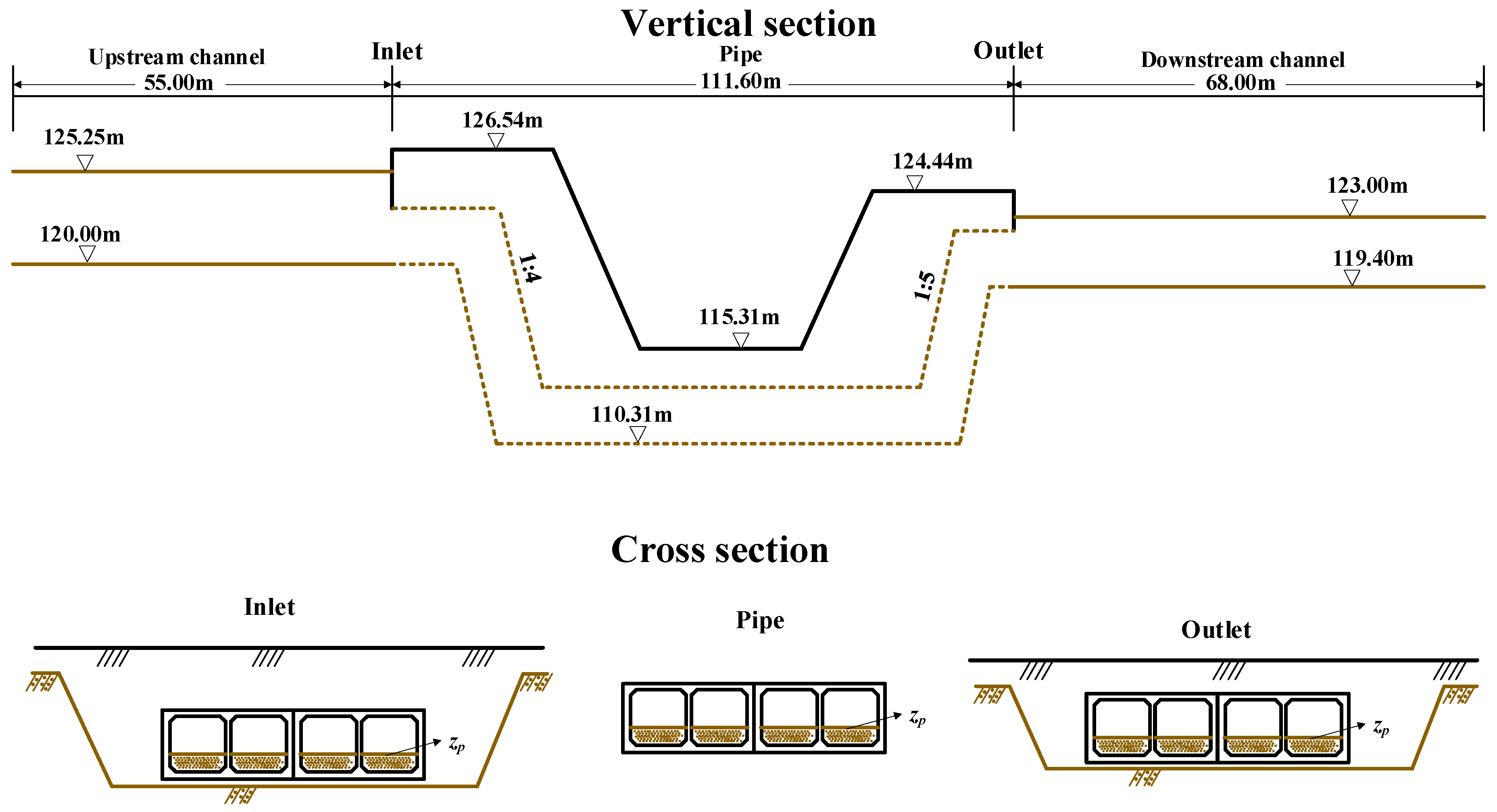
This study is targeted to the inverted siphon—A typical river-canal crossing structure. The inverted siphon, located on the intersection between main trunk canal of Central Route of the South-to-North Water Diversion Project and Meihe tributary, is taken as an illustrated case study. The drainage area of Meihe tributary is 10.80 km2, the longest length from the outlet of the main river to watershed outline is 5 km, and the average slope for the longest path is 0.017. The inverted siphon consists of pipe section, upstream channel and downstream channel sections, as shown in Figure 3. The upstream channel and downstream channel sections are the trapezoidal open channels and the lengths are 55 m and 68 m, respectively. The pipe section includes four 3 × 3 m2 square barrels, which have equal heights at the entrance. The horizontal projection length of each pipeline is 111.6 m, and the slopes of the rising and descending legs are 1:5 and 1:4, respectively. Since there is no gate control of the pipelines, the four pipelines operate simultaneously. The peak discharges for a 50-year return period of flood design criterion and 200-year flood check criterion are 209 m3/s and 294 m3/s, respectively.
3.2. Parameter Uncertainty Description
In the flood risk analysis of the inverted siphon, the parameter uncertainties in the integrated model, including rainfall module (, Cv, and γ), runoff generation module (m), runoff concentration module (u), and hydraulic module (nc, zp), are considered. The distribution and feasible range of the parameters are listed in Table 1.
3.2.1. Mean Value () and Variation Coefficient (Cv) for the Maximum 24-h Rainfall
According to the “Atlas of the Design Storm and Flood for the Medium and Small-Sized Basins in Henan Province” edited in 1984, the mean value and variation coefficient for the maximum 24-h are 100 and 0.55, respectively. However, they are both closely related to the length of the rainfall data. At the beginning of the design stage for South to North Water Diversion Project, the statistical rainfall parameters for 24 rain gauge stations, which are distributed on different rivers but along the main trunk canal, are validated with the rainfall data prolonged to 2000. The results show that the mean value ranges within −10%–10% of the designed value and Cv ranges within −0.05–0.05. Regardless of the impact of human activities, it is assumed that the statistical parameters change within the above ranges. That is, the ranges of and Cv are 90–110 and 0.5–0.6, respectively, and and Cv are assumed to be uniformly distributed.
3.2.2. The Rainfall Diminishing Exponent (γ), Runoff Concentration Parameter (m) and the Mean Filtration Rate (u)
Statistic parameters of γ, m, and u are obtained from the corresponding contour map in “Atlas of the Design Storm and Flood for the Medium and Small-Sized Basins in Henan Province”. The uncertainties in these parameters are caused by observation. The ranges for γ, m and u are 0.75–0.80, 2–5, and 0.95–1.05, respectively, by the upper and lower contour curve evaluation. γ, m and u are assumed to follow the uniform distribution.
3.2.3. The Roughness Coefficient (nc)
The roughness coefficient of the pipe for the inverted siphon (nc) changes with sediment deposition. The more sediments, the greater roughness coefficient. The roughness coefficient can reach as large as 0.020 according to the empirical data [24]. However, the inverted siphon was designed according to a fixed value, i.e., 0.014. Therefore, we consider the uncertainty of nc within range 0.014–0.020 obeying a uniform distribution.
3.2.4. The Initial Deposition Height of Sediment (zp)
The initial deposition height of sediment in the model is set at the beginning of the flood process. It can be as large as the pipe width, 3 m in this study. zp is typically small with the larger probability, while small probability corresponds to a large zp. Thus, the truncated normal distribution, which is widely used when there is little information about the distribution, is assumed for zp within range 0–3.
4. Results and Discussion
4.1. RSA Results
The parameters in the integrated model, listed in Table 1, are assumed to be independent, and Latin Hypercube sampling method [30] is used. It is noted that the parameters of the hydraulic model (roughness coefficient and initial deposition height) for each conduit (the culvert consists of four squared conduits) are set to be identical. The sample size is 100,000, and one sample includes all parameters values that are randomly assigned. The distributions of runoff concentration time and peak discharge are shown in Figure 4. As can be seen, the peak discharge considering the uncertainties of parameters are all larger than the original designed value, 294 m3/s.
The parameters sets are divided into two subsets in terms of the inverted siphon failure (i.e., non-behavioral) or operation (behavioral), with cumulative distributions shown in Figure 3. The behavioral sample (SB) is that no water flows into the canal, i.e., the water level at the water intake is smaller than the embankment crest elevation. In contrast, the non-behavioral sample (SNB) is that water flows into the canal, i.e., the water level at the water intake is higher than the crest elevation. In Figure 3, the diagonal line (D-line) represents the parameter has a uniform distribution and the model is not sensitive to this parameter in terms of the chosen likelihood measure. Any deviation from the “D-line” shows a non-uniform distribution and the model is sensitive to this parameter. The larger distance between the SB and SNB indicates more sensitive range of this parameter.
As shown in Figure 5, all parameters exhibit an obvious shift. In addition, the SNB curve for all the parameters except zp is close to “D-line”, indicating that the effects of parameters within the whole range on the failure of the inverted siphon are almost identical. The cumulative distributions for the mean rainfall (), variation coefficient (Cv), rainfall diminishing exponent (γ), runoff concentration parameter (m) and the roughness coefficient (nc), show that the values at the lower end of the tested ranges contribute to the greatest number of behaviors, i.e., lower value of these parameters lead to lower flood risk of the inverted siphon. Conversely, the greatest number of behaviors occurs at the higher end of the range for mean filtration rate (u). For initial deposition height (zp), the greatest number of behaviors and non-behaviors comes from values at the lower end of the range. Meanwhile, the initial deposition height (zp) has the least impact on flood risk of the inverted siphon, with the smallest shift from the straight line in comparison with the others.
Each parameter sensitivity is tested by the two-sample Kolmogorov–Smirnov (K-S) test method with the confidential level of 95%. Results show that the mean rainfall () is most sensitive, followed by the roughness coefficient (nc). Furthermore, the other parameters related with the rainfall, i.e., variation coefficient (Cv), rainfall diminishing exponent (γ), are more sensitive, and thus, the rainfall is the most important factor for the flood risk of the inverted siphon. The roughness coefficient (nc) is related with the conveyance capacity of the pipe, thus the conveyance capacity of the pipe also is the most important factor for the flood risk of the inverted siphon.
4.2. Soboĺ Sensitivity Analysis Results
The first-order and total-order sensitivity indices of seven parameters are shown in Figure 4. The black bars represent the first-order index values, which measure the individual parameter contributions to the duration and volume of flood overtopping. The white bars represent the interactive indices, which demonstrate the total interactive contribution of one parameter with all other parameters. The parameter is identified as sensitive when total-order sensitivity index is larger than 0.1.
As can be seen in Figure 6, the total-order index for roughness coefficient (nc), mean rainfall (), variation coefficient (Cv) and rainfall diminishing exponent (γ), are all larger than 0.1, i.e., sensitive parameters for flood overtopping duration and volume. Parameters m and u, which are related with runoff generation and concentration, are not sensitive. The reason is that flood hydrograph, flood volume, and the conveyance capacity of the pipe are the most important factors for the flood overtopping. A larger flood volume or smaller conveyance capacity leads to more water retained at the inlet, and thus leads to a larger risk of flood overtopping. The magnitude of rainfall is the most important factor of flood volume and flood hydrograph. Thus, the parameters related with the magnitude of rainfall and conveyance capacity are sensitive. The initial deposition height (zp) is sensitive for the flood overtopping duration, but it is not sensitive for the flood overtopping volume.
The results of the overtopping duration show that obtains the largest value of total-order index, followed by nc. These two parameters determine the magnitude of rainfall and the water conveyance capacity of the pipe, respectively. Therefore, the result indicates that rainfall and the water conveyance capacity of the pipe both have a great impact on the overtopping duration in the inverted siphon. The results of the flood overtopping volume show the total-order index for , Cv, γ as well as nc are sensitive parameters. , Cv and γ determine the runoff volume, which is the input of the inverted siphon, while nc determines the flood volume transported.
Figure 6 show the interaction between zp and other parameters is strong, and the interaction for the flood overtopping volume is weaker than the flood overtopping duration. The interaction between any two parameters is shown in Figure 7. As can be seen in Figure 7a, the sum of the second-order index between zp and other parameters is the largest, and the interaction between zp and m is strongest for the flood overtopping duration. As for flood overtopping volume, the sum of second-order index between nc and other parameters is largest. However, Figure 6b shows that the total interactions of zp is larger than that of nc, which indicates that higher order interactions (third-order, four-order, etc.) exist between zp and other parameters. The second-order index value for nc and γ is strongest, followed by the value for nc and , indicating that the interaction between nc and γ, nc and are strong. This is because is the most important factor that determines the flood volume, and a larger result in a larger flood. A larger γ results in a larger runoff generation under the same magnitude of rainfall, and a larger results in a larger and thus a larger peak discharge and flood volume, while a larger nc results in a smaller conveyance capacity.
In conclusion, results of RSA and Soboĺ sensitivity analysis both indicate that the mean rainfall and roughness coefficient of the pipe are two important parameters, which determine the rainfall and water conveyance capacity of the siphon pipe, respectively. These results demonstrate that lower value of the mean rainfall or roughness coefficient of the pipe lead to lower flood risk of the inverted siphon. Thus, the effective measures for reducing the flood risk of the inverted siphon to clean the inverted siphon periodically, i.e., reduce the roughness coefficient of pipe.
5. Conclusions
This paper investigated, by using an integrated system coupling the hydrology and hydraulic models, the impact of rainfall, sediments and pipe roughness coefficient on the failure of inverted siphon through RSA and Soboĺ sensitivity analysis. The flood risk of the inverted siphon is evaluated by the flood overtopping duration and volume. The conclusions are summarized as follows:
(1) RSA and Soboĺ sensitivity analyses both indicate the mean rainfall and the roughness coefficient of the pipe are most sensitive for the flood risk of the inverted siphon. These results imply that lower value of the mean rainfall or roughness coefficient of the pipe lead to lower flood risk of the inverted siphon. Thus, periodically cleaning the inverted siphon is an effective measure for reducing the flood risk of the inverted siphon, i.e., reduce the roughness coefficient of pipe.
(2) The RSA identifies the sensitivity range of safety and failure for the inverted siphon. Effects of all parameters except initial deposition height throughout the feasible range on the failure of the inverted siphon are almost identical. For the safety of the inverted siphon, the smaller values of variation coefficient, rainfall diminishing exponent, runoff concentration parameter, and roughness coefficient of pipe, the more safety of the inverted siphon. For the mean filtration, a higher value leads to the more security of the inverted siphon.
(3) Soboĺ sensitivity analysis reveals the individual and interactive effects of the parameters. The effects of all parameters on flow overtopping duration and volume all parameters are all dominated by the individual effects. For the flood overtopping duration, the interactions between the initial deposition height and other parameters are high, with the largest interaction between initial deposition height and confluence coefficient. For flood overtopping volume, the interaction between rainfall model parameters and hydraulic model parameters are both significant.
Acknowledgments
This research was supported by the National Key Research and Development Program of China (Grant No. 2016YFC0402203) and partly funded by the National Science and Technology Major Project (Grant No. 2014ZX03005001) and National Science Foundation of China (Grant No. 91547116).
Author Contributions
Wei Ding and Haixing Liu conceived and designed the experiments; Sifan Jin performed the experiments; SiFan Jin, Haixing Liu and Wei Ding analyzed the data; Hua Shang and Guoli Wang contributed reagents/materials/analysis tools; Sifan Jin wrote the paper.
Conflicts of Interest
The authors declare no conflict of interest.
References
- Liu, C.; Zheng, H. South-to-north Water Transfer Schemes for China. Int. J. Water Resour. Dev. 2002, 18, 453–471. [Google Scholar] [CrossRef]
- Koutsoyiannis, D. Scale of water resources development and sustainability: Small is beautiful, large is great. Hydrol. Sci. J. 2011, 56, 553–575. [Google Scholar] [CrossRef]
- Tyralis, H.; Aristoteles, T.; Delichatsiou, A.; Mamassis, N.; Koutsoyiannis, D. A perpetually interrupted interbasin water transfer as a modern Greek drama: Assessing the Acheloos to Pinios interbasin water transfer in the context of integrated water resources management. Open Water J. 2017, 4, 11. [Google Scholar]
- Zhang, Q. The South-to-North Water Transfer Project of China: Environmental Implications and Monitoring Strategy. JAWRA J. Am. Water Resour. Assoc. 2009, 45, 1238–1247. [Google Scholar] [CrossRef]
- Tang, C.; Yi, Y.; Yang, Z.; Cheng, X. Water pollution risk simulation and prediction in the main canal of the South-to-North Water Transfer Project. J. Hydrol. 2014, 519, 2111–2120. [Google Scholar] [CrossRef]
- Wei, G.; Zhang, C.; Li, Y.; Liu, H.; Zhou, H. Source identification of sudden contamination based on the parameter uncertainty analysis. J. Hydroinform. 2016, 18, 919–927. [Google Scholar]
- Pappenberger, F.; Beven, K.J.; Ratto, M.; Matgen, P. Multi-method global sensitivity analysis of flood inundation models. Adv. Water Resour. 2008, 31, 1–14. [Google Scholar] [CrossRef]
- Van Griensven, A.; Meixner, T.; Grunwald, S.; Bishop, T.; Diluzio, M.; Srinivasan, R. A global sensitivity analysis tool for the parameters of multi-variable catchment models. J. Hydrol. 2006, 324, 10–23. [Google Scholar] [CrossRef]
- Chu, J.; Zhang, C.; Fu, G.; Li, Y.; Zhou, H. Improving multi-objective reservoir operation optimization with sensitivity-informed dimension reduction. Hydrol. Earth Syst. Sci. 2015, 19, 3557–3570. [Google Scholar] [CrossRef] [Green Version]
- Song, X.; Zhang, J.; Zhan, C.; Xuan, Y.; Ye, M.; Xu, C. Global sensitivity analysis in hydrological modeling: Review of concepts, methods, theoretical framework, and applications. J. Hydrol. 2015, 523, 739–757. [Google Scholar] [CrossRef]
- Ruppert, D.; Shoemaker, C.A.; Wang, Y.; Li, Y.; Bliznyuk, N. Uncertainty Analysis for Computationally Expensive Models with Multiple Outputs. J. Agric. Biol. Environ. Stat. 2012, 17, 623–640. [Google Scholar] [CrossRef]
- Gan, Y.; Duan, Q.; Gong, W.; Tong, C.; Sun, Y.; Chu, W.; Ye, A.; Miao, C.; Di, Z. A comprehensive evaluation of various sensitivity analysis methods: A case study with a hydrological model. Environ. Model. Softw. 2014, 51, 269–285. [Google Scholar] [CrossRef]
- Soboĺ, I. Quasi-Monte Carlo methods. Prog. Nucl. Energy 1990, 24, 55–61. [Google Scholar] [CrossRef]
- Saltelli, A.; Tarantola, S. On the Relative Importance of Input Factors in Mathematical Models. J. Am. Stat. Assoc. 2002, 97, 702–709. [Google Scholar] [CrossRef]
- Fu, G.; Kapelan, Z.; Reed, P. Reducing the complexity of multiobjective water distribution system optimization through global sensitivity analysis. J. Water Resour. Plan. Manag. 2012, 138, 196–207. [Google Scholar] [CrossRef]
- Zhang, C.; Chu, J.; Fu, G. Soboĺ sensitivity analysis for a distributed hydrological model of Yichun River Basin, China. J. Hydrol. 2013, 480, 58–68. [Google Scholar] [CrossRef] [Green Version]
- Spear, R.C.; Hornberger, G.M. Eutrophication in peel inlet—II. Identification of critical uncertainties via generalized sensitivity analysis. Water Res. 1980, 14, 43–49. [Google Scholar] [CrossRef]
- Beven, K.; Binley, A. The future of distributed models: Model calibration and uncertainty prediction. Hydrol. Process. 1992, 6, 279–298. [Google Scholar] [CrossRef]
- Pappenberger, F.; Iorgulescu, I.; Beven, K.J. Sensitivity analysis based on regional splits and regression trees (SARS-RT). Environ. Model. Softw. 2006, 21, 976–990. [Google Scholar] [CrossRef]
- Saltelli, A.; Tarantola, S.; Chan, K.-S. A quantitative model-independent method for global sensitivity analysis of model output. Technometrics 1999, 41, 39–56. [Google Scholar] [CrossRef]
- Tang, Y.; Reed, P.; Van Werkhoven, K.; Wagener, T. Advancing the identification and evaluation of distributed rainfall-runoff models using global sensitivity analysis. Water Resour. Res. 2007, 43. [Google Scholar] [CrossRef]
- Yang, J. Convergence and uncertainty analyses in Monte-Carlo based sensitivity analysis. Environ. Model. Softw. 2011, 26, 444–457. [Google Scholar] [CrossRef]
- Massmann, C.; Holzmann, H. Analysis of the behavior of a rainfall–runoff model using three global sensitivity analysis methods evaluated at different temporal scales. J. Hydrol. 2012, 475, 97–110. [Google Scholar] [CrossRef]
- Wu, C. Hydraulics, 4th ed.; Higher Education Press: Beijing, China, 2008. (In Chinese) [Google Scholar]
- Chen, J.; Zhang, G. Storm-Flood Computation of Small Watershed; China Conservancy and Hydropower Press: Beijing, China, 1985. (In Chinese) [Google Scholar]
- Mulvaney, T.J. On the Use of Self-Registering Rain and Flood Gauges in Making Observations of the Relations of Rain Falland Flood Discharges in a Given Catchment, Proceedings of the Institute of Civil Engineers of Ireland, Session 1850-1; Transactions of the Institution of Civil Engineers of Ireland: Dublin, Ireland, 1851; Volume 4, pp. 18–33. [Google Scholar]
- Guo, J. Logarithmic matching and its applications in computational hydraulics and sediment transport. J. Hydraul. Res. 2002, 40, 555–565. [Google Scholar] [CrossRef]
- Zhu, L.; Cheng, N. Settlement of Sediment Particles; Nanjing Hydraulic Research Institute: Nanjing, China, 1993. (In Chinese) [Google Scholar]
- Wasp, E.J.; Kenny, J.P.; Gandhi, R.L. Solid-liquid Flow Slurry Pipeline Transportation; Ser. Bulk Materials Handling; Trans Tech Publications: Zurich, Switzerland, 1977; Volume 1, p. 4. [Google Scholar]
- McKay, M.D.; Beckman, R.J.; Conover, W.J. A comparison of three methods for selecting values of input variables in the analysis of output from a computer code. Technometrics 2000, 42, 55–61. [Google Scholar] [CrossRef]
Figure 1.
Flow chart of the models.
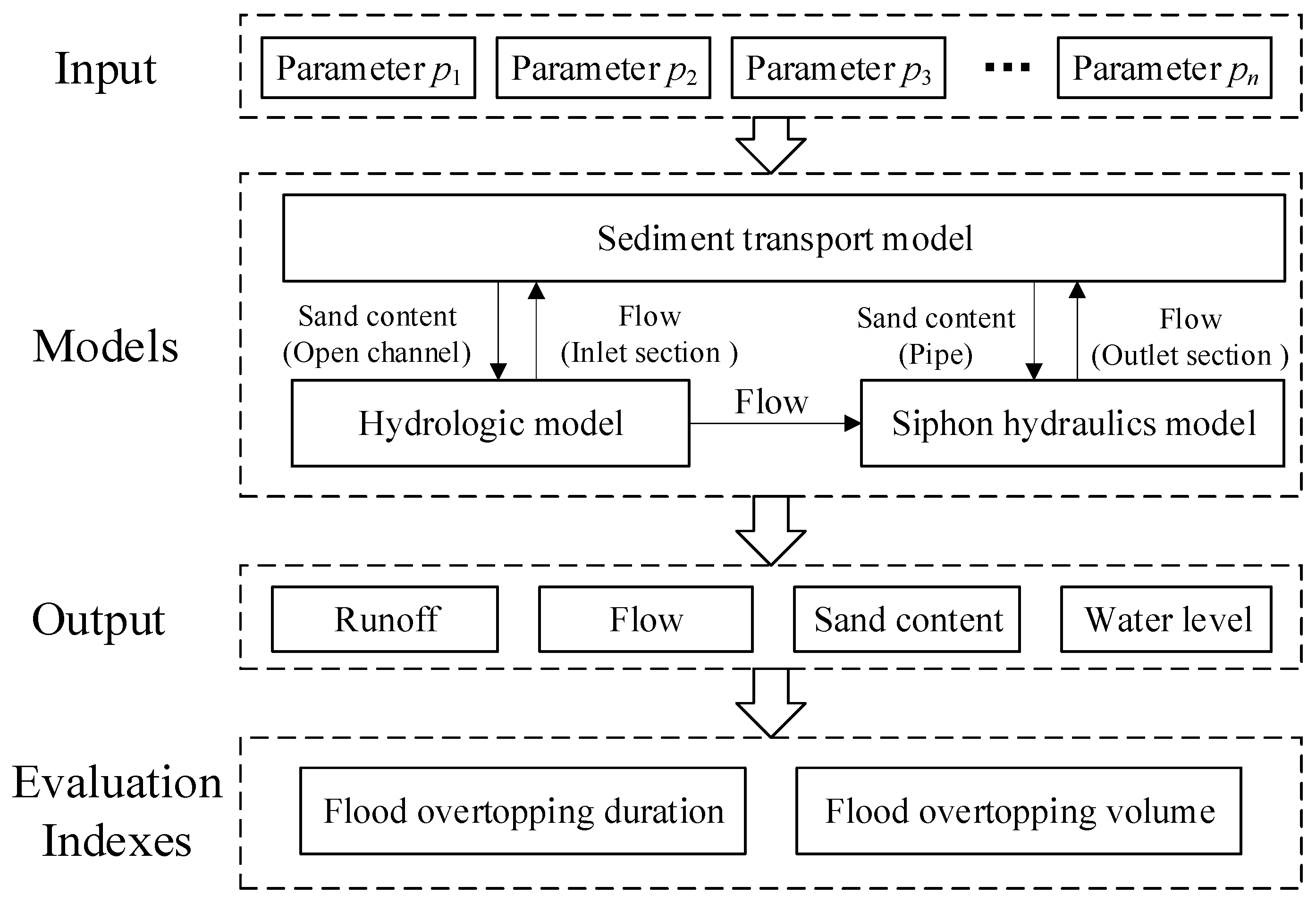
Figure 2.
The sketch map of the study area.
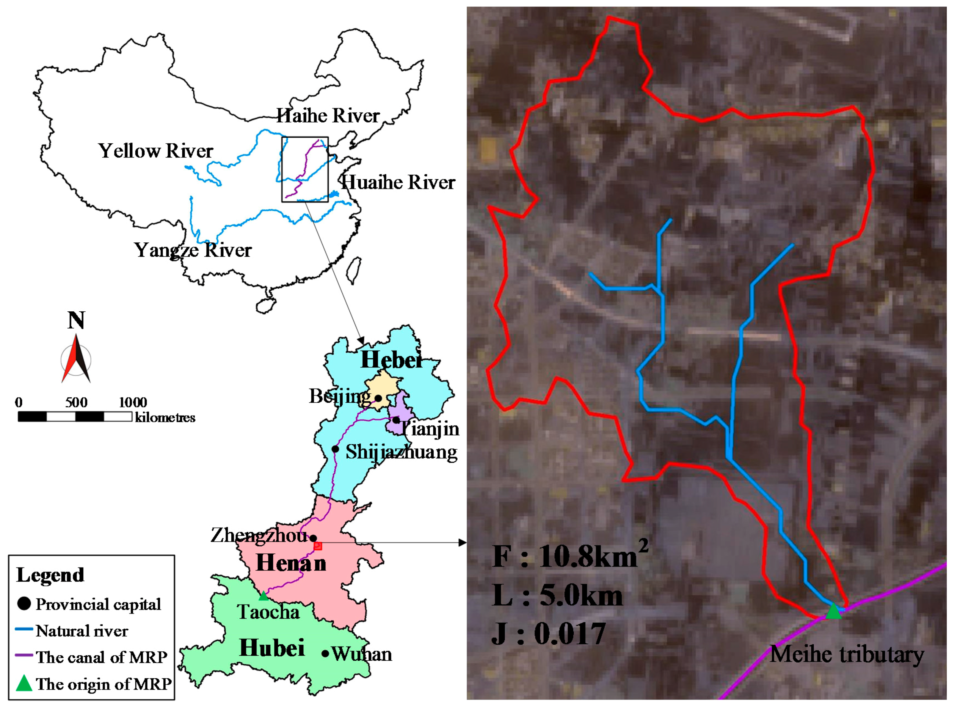
Figure 3.
The schematic diagram of the inverted siphon.

Figure 4.
The distribution of runoff concentration time and peak discharge. (a) The distribution of runoff concentration time; (b) The distribution of peak discharge.
Figure 4.
The distribution of runoff concentration time and peak discharge. (a) The distribution of runoff concentration time; (b) The distribution of peak discharge.

Figure 5.
Cumulative distribution of the seven parameters with regard to failure of the inverted siphon. SB and SNB represent the behavioral and non-behavioral groups, respectively. (a) Cumulative distribution of mean rainfall; (b) Cumulative distribution of variation coefficient; (c) Cumulative distribution of rainfall diminishing exponent; (d) Cumulative distribution of runoff concentration parameter; (e) Cumulative distribution of mean filtration rate; (f) Cumulative distribution of roughness coefficient; (g) Cumulative distribution of initial deposition height.
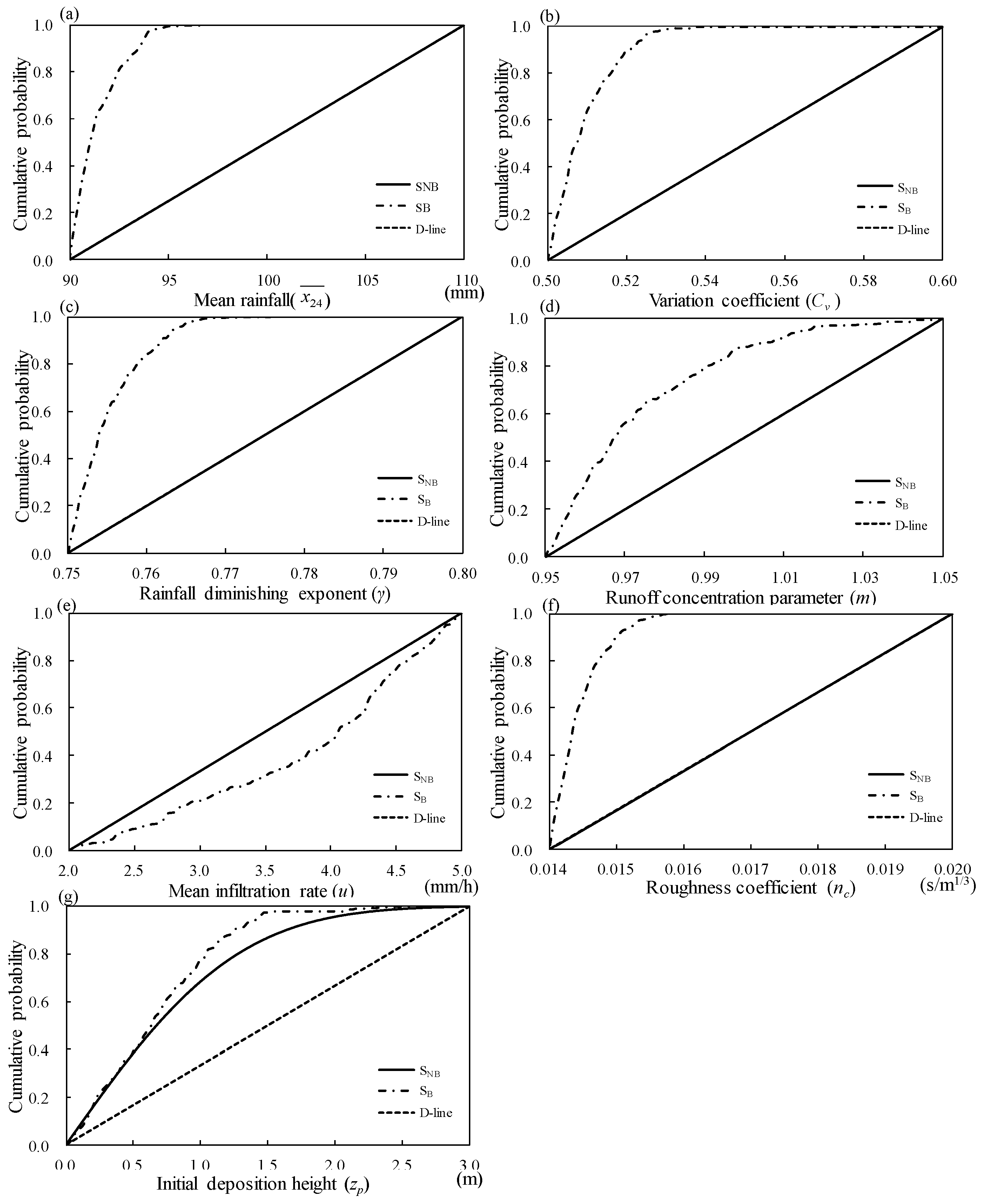
Figure 6.
The first-order sensitivity and total-order sensitivity of parameters. (a) The first-order sensitivity and total-order sensitivity of parameters for flood overtopping duration; (b) The first-order sensitivity and total-order sensitivity of parameters for flood overtopping volume.
Figure 6.
The first-order sensitivity and total-order sensitivity of parameters. (a) The first-order sensitivity and total-order sensitivity of parameters for flood overtopping duration; (b) The first-order sensitivity and total-order sensitivity of parameters for flood overtopping volume.

Figure 7.
The interaction between each two parameters. (a) The interaction between each two parameters for flood overtopping duration; (b) The interaction between each two parameters for flood overtopping volume.
Figure 7.
The interaction between each two parameters. (a) The interaction between each two parameters for flood overtopping duration; (b) The interaction between each two parameters for flood overtopping volume.


Table 1.
Parameters studied for the sensitivity analysis.
| Model Response | Parameter | Description | Range | Distribution | Unit |
|---|---|---|---|---|---|
| Rainfall | Mean annual maximum rainfall in 24 h | 90–110 | uniform | mm | |
| Cv | Variation coefficient of annual maximum rainfall in 24 h | 0.5–0.6 | uniform | -- | |
| γ | Rainfall diminishing exponent | 0.75–0.80 | uniform | -- | |
| Runoff | u | Mean infiltration rates | 2–5 | uniform | mm/h |
| m | Confluence coefficient | 0.95–1.05 | uniform | -- | |
| Conduit flow | nc | Roughness coefficient of the pipe | 0.014–0.020 | uniform | -- |
| zp | Initial deposition height | 0–3 | truncated normal | m |
© 2018 by the authors. Licensee MDPI, Basel, Switzerland. This article is an open access article distributed under the terms and conditions of the Creative Commons Attribution (CC BY) license (http://creativecommons.org/licenses/by/4.0/).
Share and Cite
MDPI and ACS Style
Jin, S.; Liu, H.; Ding, W.; Shang, H.; Wang, G. Sensitivity Analysis for the Inverted Siphon in a Long Distance Water Transfer Project: An Integrated System Modeling Perspective. Water 2018, 10, 292. https://doi.org/10.3390/w10030292
AMA Style
Jin S, Liu H, Ding W, Shang H, Wang G. Sensitivity Analysis for the Inverted Siphon in a Long Distance Water Transfer Project: An Integrated System Modeling Perspective. Water. 2018; 10(3):292. https://doi.org/10.3390/w10030292
Chicago/Turabian StyleJin, Sifan, Haixing Liu, Wei Ding, Hua Shang, and Guoli Wang. 2018. "Sensitivity Analysis for the Inverted Siphon in a Long Distance Water Transfer Project: An Integrated System Modeling Perspective" Water 10, no. 3: 292. https://doi.org/10.3390/w10030292
Note that from the first issue of 2016, this journal uses article numbers instead of page numbers. See further details here.