Improving the Computational Performance of an Operational Two-Dimensional Real-Time Flooding Forecasting System by Active-Cell and Multi-Grid Methods in Taichung City, Taiwan


Abstract
:
1. Introduction
2. Materials and Methods
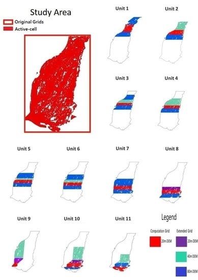
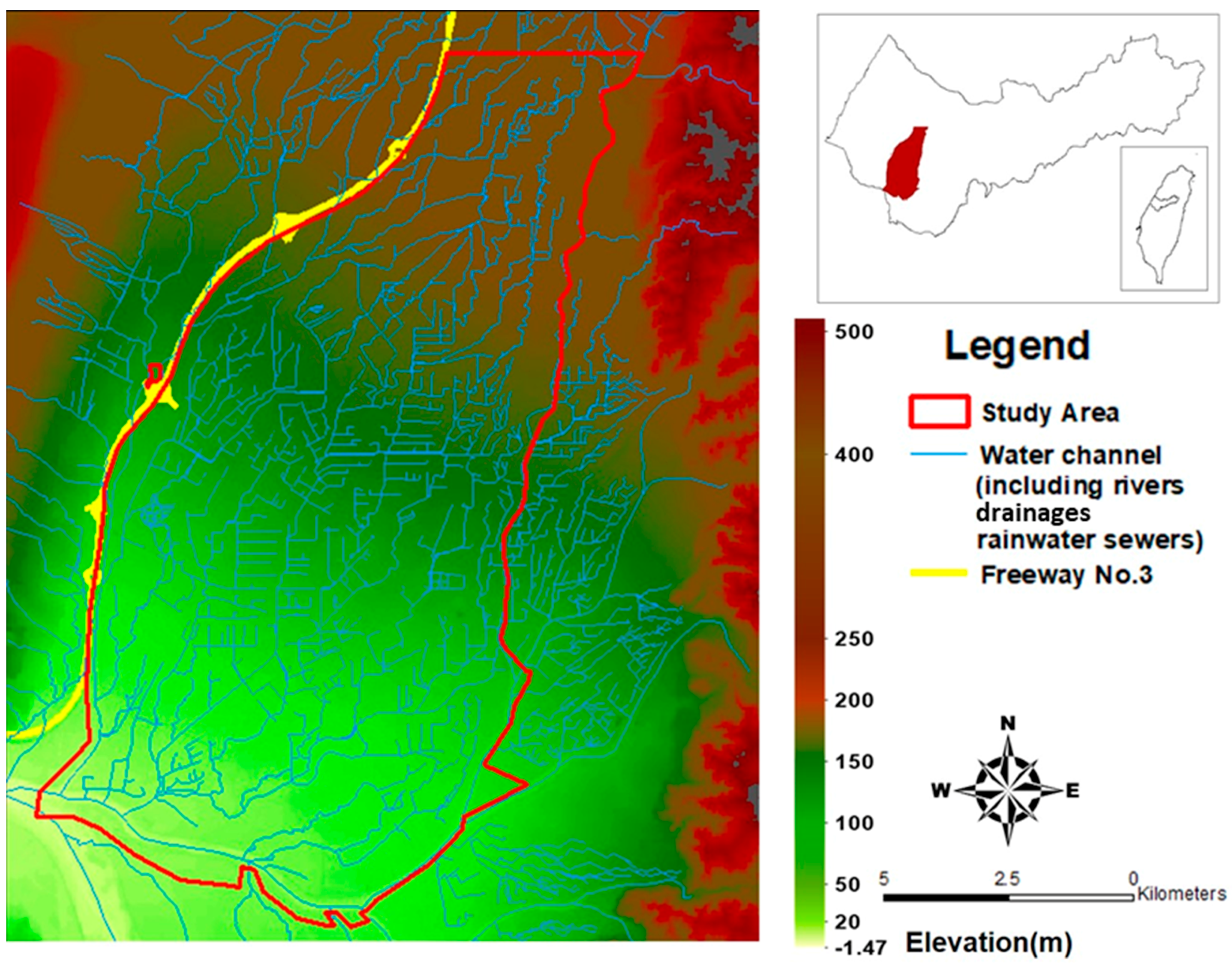
2.1. Study Area
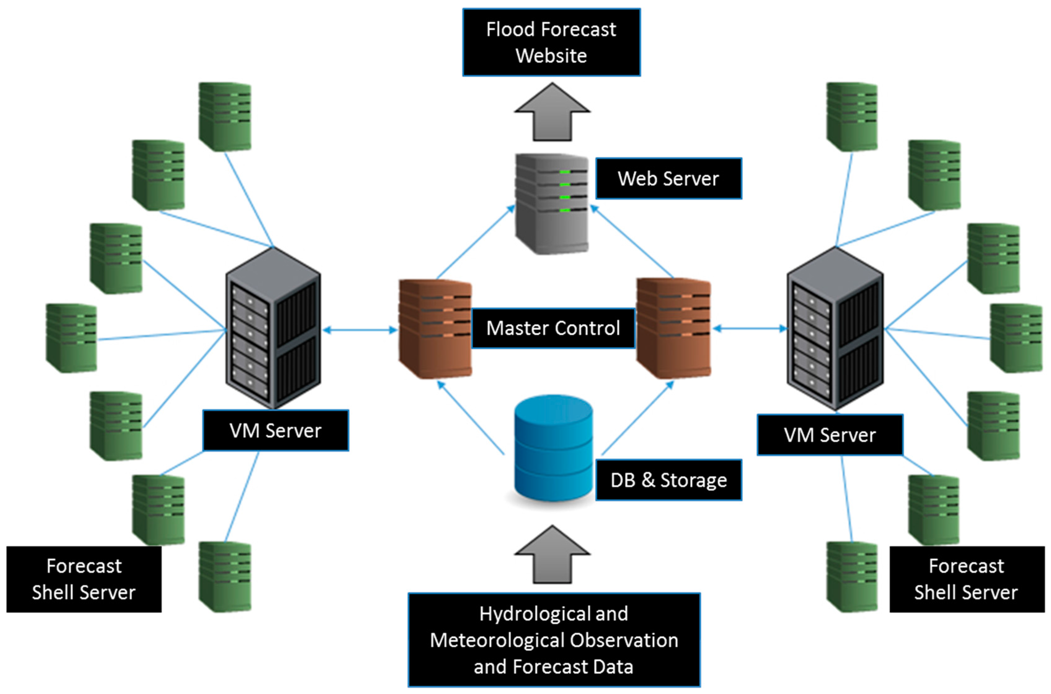
2.2. Delft-FEWS
2.3. SOBEK Model
2.4. Grid Methods
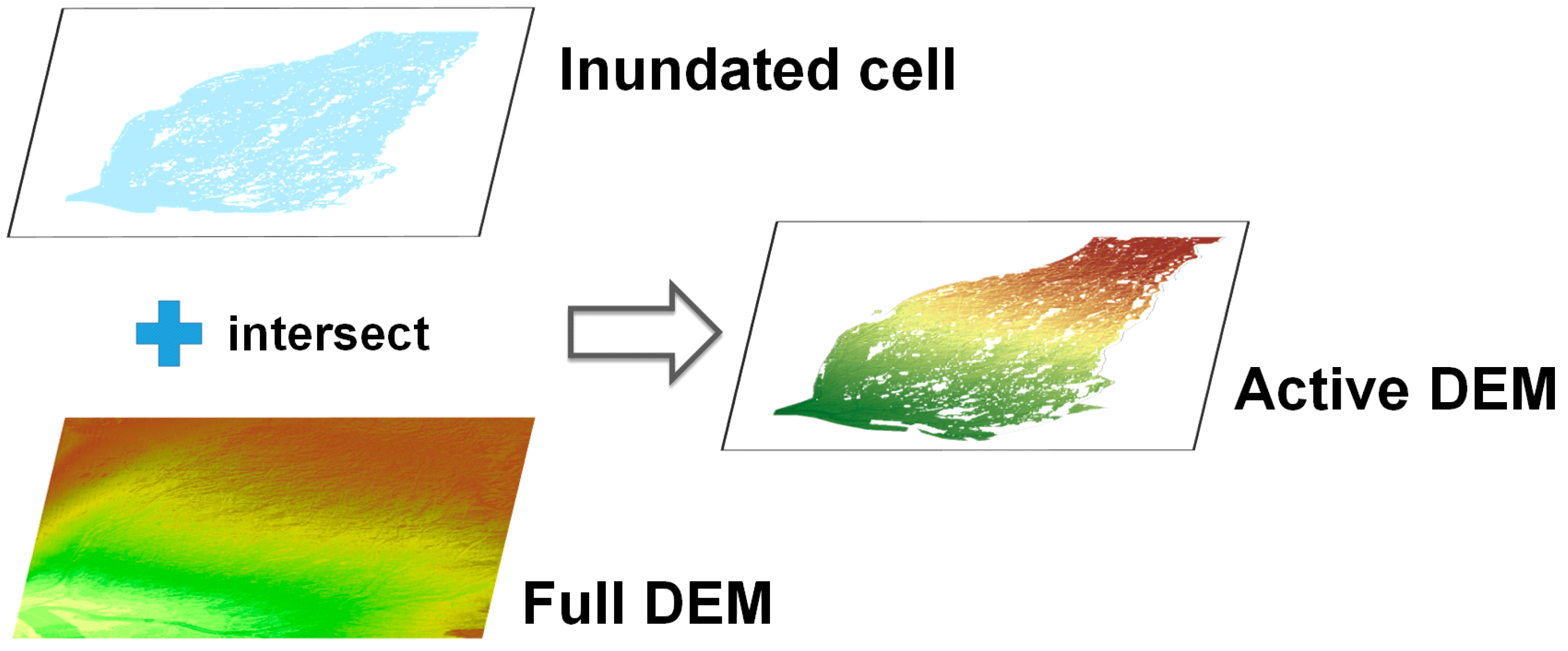
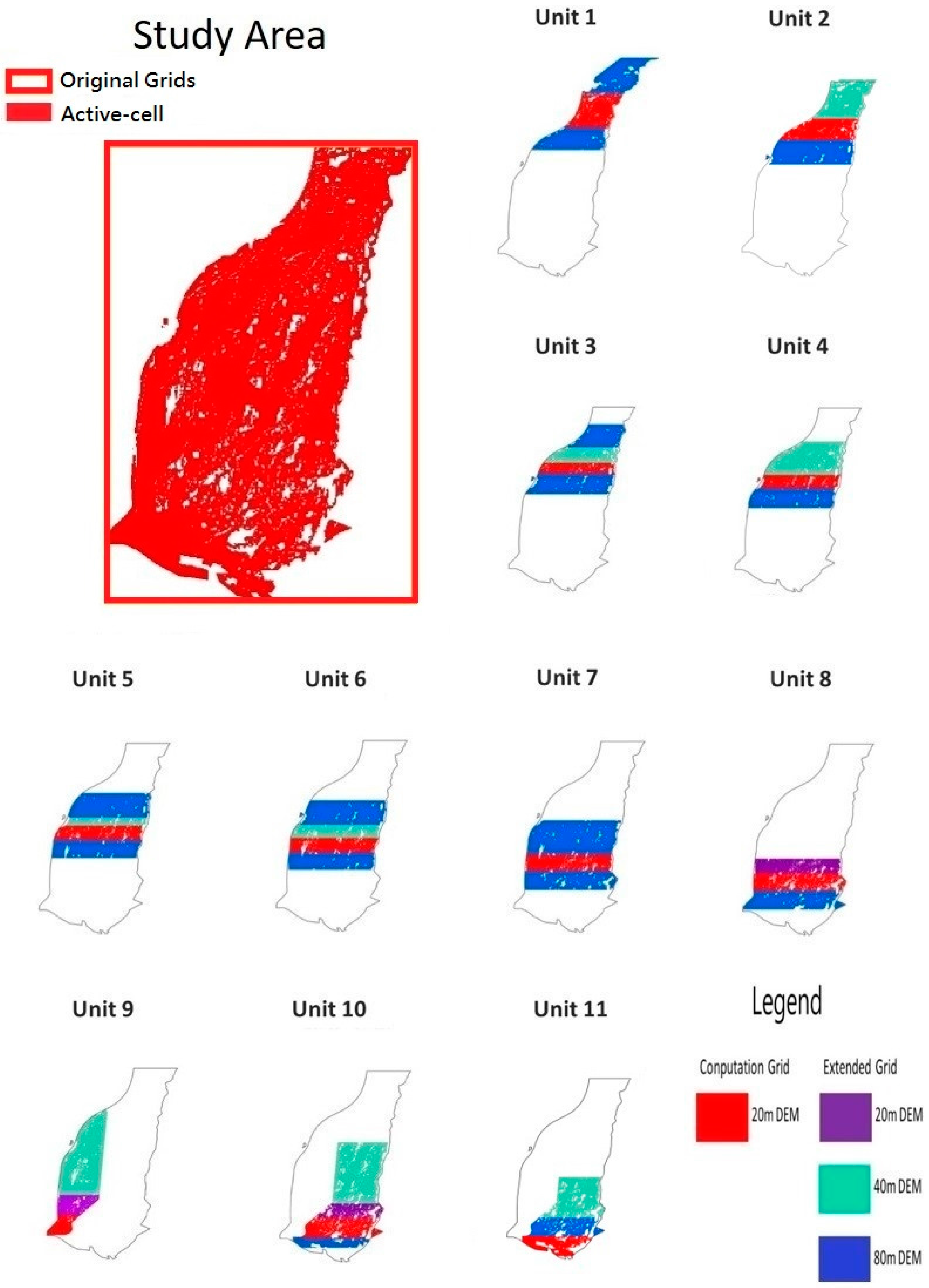
2.4.1. Active-Cell
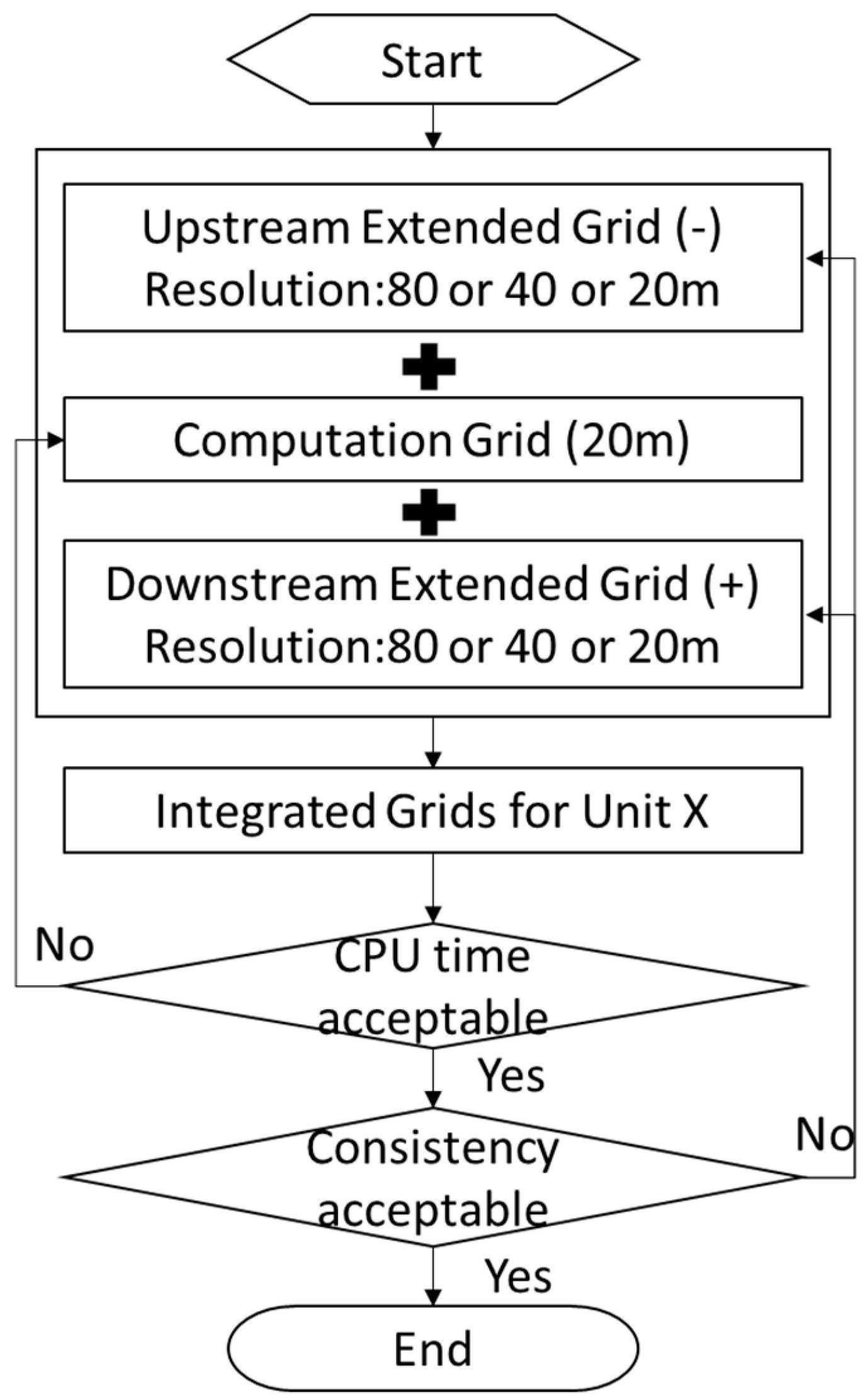
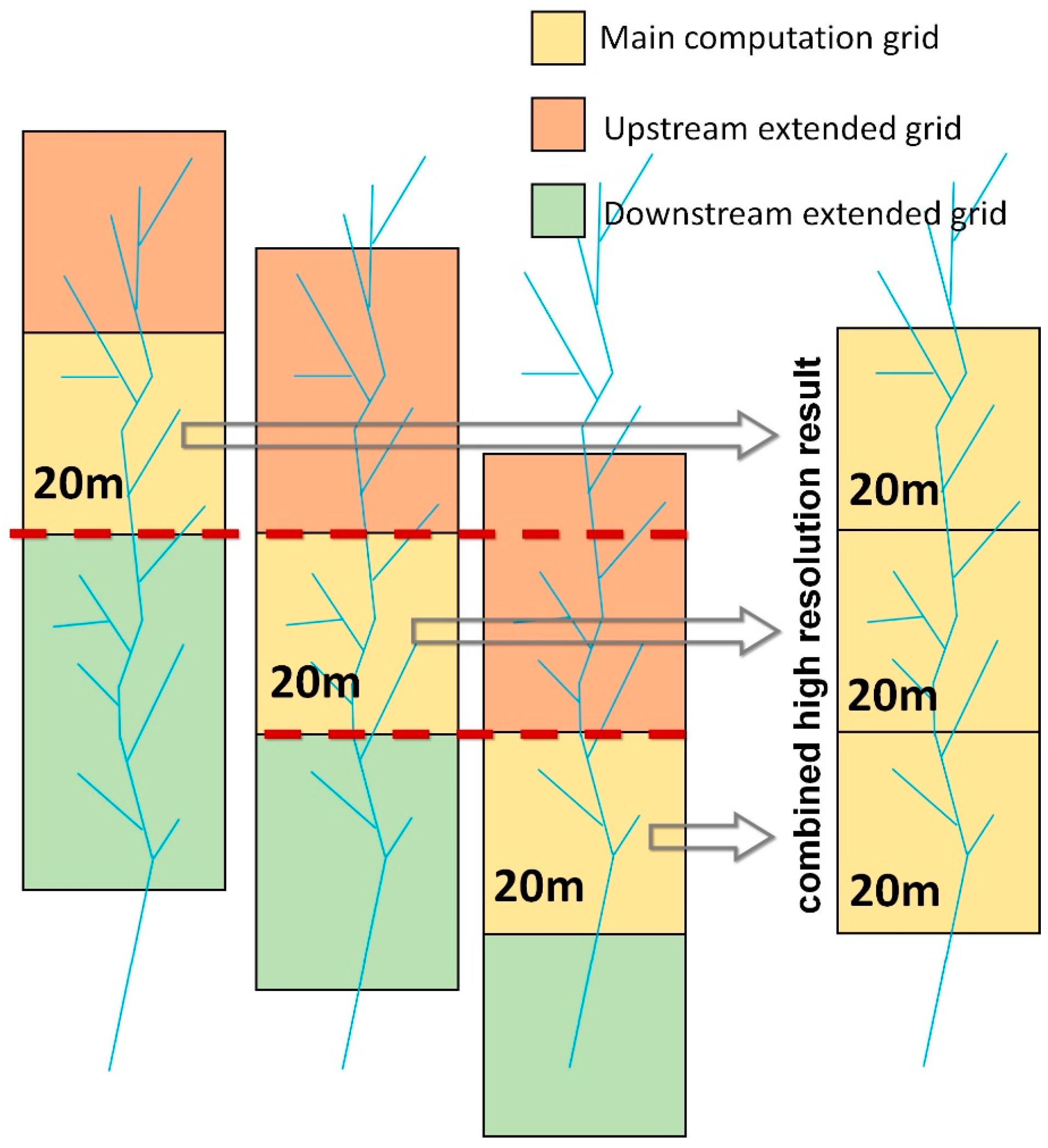
2.4.2. Multi-Grid
2.5. Results Verification
3. Results and Discussion
3.1. Active-Cell
3.2. Multi-Grid
4. Conclusions
Acknowledgments
Author Contributions
Conflicts of Interest
References
- Werner, M.; Cranston, M.; Harrison, T.; Whitfield, D.; Schellekens, J. Recent developments in operational flood forecasting in england, wales and scotland. Meteorol. Appl. 2009, 16, 13–22. [Google Scholar] [CrossRef]
- Vehviläinen, B.; Huttunen, M. Hydrological Forecasting and Real Time Monitoring in Finland: The Watershed Simulation and Forecasting System (WSFS); Finnish Environment Institute: Helsinki, Finland, 2001. [Google Scholar]
- Kirby, D. Flood integrated decision support system for melbourne (fidss). In Proceedings of the 2015 Floodplain Management Association National Conference, Brisbane, Australia, 19–22 May 2015. [Google Scholar]
- Johnell, A.; Lindström, G.; Olsson, J. Deterministic evaluation of ensemble streamflow predictions in sweden. Hydrol. Res. 2007, 38, 441–450. [Google Scholar] [CrossRef]
- Krajewski, W.F.; Ceynar, D.; Demir, I.; Goska, R.; Kruger, A.; Langel, C.; Mantilla, R.; Niemeier, J.; Quintero, F.; Seo, B.-C. Real-time flood forecasting and information system for the state of iowa. Bull. Am. Meteorol. Soc. 2017, 98, 539–554. [Google Scholar] [CrossRef]
- Tospornsampan, M.J.; Malone, T.; Katry, P.; Pengel, B.; An, H.P. Fmmp component 1 short and medium-term flood forecasting at the regional flood management and mitigation centre. Mekong River Comm. 2009, 7, 155–164. [Google Scholar]
- Chang, C.-H. Establishment and Application of Radar Data and Hydrologic Models in an Integrated Platform of Hydrometeorology Observation; Water Resources Agency: Taichung, Taiwan, 2013.
- Chang, C.-H. The Development of Value-Add Application for Rainfall Rader Data and Multiple Hydrology Models Based on Fews_Taiwan; Water Resources Agency: Taichung, Taiwan, 2014.
- Syme, W.; Pinnell, M.; Wicks, J. Modelling flood inundation of urban areas in the uk using 2d/1d hydraulic models. In Proceedings of the 8th National Conference on Hydraulics in Water Engineering, Gold Coast, Australia, 13–16 July 2004; The Institution of Engineers: Gold Coast, Australia, 2004. [Google Scholar]
- Chang, C.-H. Integrated Platform for Application of High-Performance 2D Inundation Simulation; Water Resources Planning Institute: Taichung, Taiwan, 2016.
- Moore, M.R. Development of a High-Resolution 1D/2D Coupled Flood Simulation of Charles City, Iowa; University of Iowa: Iowa City, ID, USA, 2011. [Google Scholar]
- Sampson, C.C.; Fewtrell, T.J.; Duncan, A.; Shaad, K.; Horritt, M.S.; Bates, P.D. Use of terrestrial laser scanning data to drive decimetric resolution urban inundation models. Adv. Water Resour. 2012, 41, 1–17. [Google Scholar] [CrossRef]
- Meesuk, V.; Vojinovic, Z.; Mynett, A.E.; Abdullah, A.F. Urban flood modelling combining top-view lidar data with ground-view sfm observations. Adv. Water Resour. 2015, 75, 105–117. [Google Scholar] [CrossRef]
- Marks, K.; Bates, P. Integration of high-resolution topographic data with floodplain flow models. Hydrol. Process. 2000, 14, 2109–2122. [Google Scholar] [CrossRef]
- Haile, A.T.; Rientjes, T. Effects of lidar dem resolution in flood modelling: A model sensitivity study for the city of Tegucigalpa, Honduras. In Proceedings of the ISPRS WG III/3, III/4, V/3 Workshop “Laser Scanning 2005”, Enschede, The Netherlands, 12–14 September 2005; Volume 3, pp. 12–14. [Google Scholar]
- Bates, P.D.; De Roo, A. A simple raster-based model for flood inundation simulation. J. Hydrol. 2000, 236, 54–77. [Google Scholar] [CrossRef]
- Liu, L.; Liu, Y.; Wang, X.; Yu, D.; Liu, K.; Huang, H.; Hu, G. Developing an effective 2-d urban flood inundation model for city emergency management based on cellular automata. Nat. Hazards Earth Syst. Sci. 2015, 15, 381–391. [Google Scholar] [CrossRef] [Green Version]
- Yu, D.; Lane, S.N. Urban fluvial flood modelling using a two-dimensional diffusion-wave treatment, part 1: Mesh resolution effects. Hydrol. Process. 2006, 20, 1541–1565. [Google Scholar] [CrossRef]
- Chen, A.S.; Evans, B.; Djordjević, S.; Savić, D.A. Multi-layered coarse grid modelling in 2d urban flood simulations. J. Hydrol. 2012, 470, 1–11. [Google Scholar] [CrossRef] [Green Version]
- Hunter, N.M.; Bates, P.D.; Horritt, M.S.; De Roo, A.; Werner, M.G. Utility of different data types for calibrating flood inundation models within a glue framework. Hydrol. Earth Syst. Sci. 2005, 9, 412–430. [Google Scholar] [CrossRef]
- Wang, J.P.; Liang, Q. Testing a new adaptive grid-based shallow flow model for different types of flood simulations. J. Flood Risk Manag. 2011, 4, 96–103. [Google Scholar] [CrossRef]
- Wang, X.; Cao, Z.; Pender, G.; Neelz, S. Numerical modelling of flood flows over irregular topography. Proc. Inst. Civ. Eng. Water Manag. 2010, 163, 255–265. [Google Scholar] [CrossRef]
- Sanders, B.F.; Schubert, J.E.; Detwiler, R.L. Parbrezo: A parallel, unstructured grid, godunov-type, shallow-water code for high-resolution flood inundation modeling at the regional scale. Adv. Water Resour. 2010, 33, 1456–1467. [Google Scholar] [CrossRef]
- Li, Z.; Wu, L.; Zhu, W.; Hou, M.; Yang, Y.; Zheng, J. A new method for urban storm flood inundation simulation with fine cd-tin surface. Water 2014, 6, 1151–1171. [Google Scholar] [CrossRef]
- Yu, D.; Lane, S.N. Urban fluvial flood modelling using a two-dimensional diffusion-wave treatment, part 2: Development of a sub-grid-scale treatment. Hydrol. Process. 2006, 20, 1567–1583. [Google Scholar] [CrossRef]
- Yu, D. Parallelization of a two-dimensional flood inundation model based on domain decomposition. Environ. Model. Softw. 2010, 25, 935–945. [Google Scholar] [CrossRef]
- Stelling, G.S. Quadtree flood simulations with sub-grid digital elevation models. Proc. Inst. Civ. Eng. 2012, 165, 567. [Google Scholar] [CrossRef]
- Dhondia, J.; Stelling, G. Application of one-dimensional-two-dimensional integrated hydraulic model for flood simulation and damage assessment. In Proceedings of the International Conference on Hydroinformatics, Cardiff, UK, 1–5 July 2002; pp. 265–276. [Google Scholar]
- Neal, J.C.; Fewtrell, T.J.; Bates, P.D.; Wright, N.G. A comparison of three parallelisation methods for 2d flood inundation models. Environ. Model. Softw. 2010, 25, 398–411. [Google Scholar] [CrossRef]
- Kalyanapu, A.J.; Shankar, S.; Pardyjak, E.R.; Judi, D.R.; Burian, S.T. Assessment of GPU computational enhancement to a 2D flood model. Environ. Model. Softw. 2011, 26, 1009–1016. [Google Scholar]
- Teng, J.; Jakeman, A.J.; Vaze, J.; Croke, B.F..; Dutta, D.; Kim, S. Flood inundation modelling: A review of methods, recent advances and uncertainty analysis. Environ. Model. Softw. 2017, 90, 201–216. [Google Scholar]
- Costabile, P.; Macchione, F. Enhancing river model set-up for 2-d dynamic flood modelling. Environ. Model. Softw. 2015, 67, 89–107. [Google Scholar] [CrossRef]
- Werner, M.; van Dijk, M.; Schellekens, J. Delft-fews: An open shell flood forecasting system. In Hydroinformatics: (in 2 Volumes, with CD-ROM); World Scientific: Singapore, 2004; pp. 1205–1212. [Google Scholar]
- Werner, M.; Heynert, K. Open model integration—A Review of practical examples in operational flood forecasting. In Proceedings of the Seventh International Conference on Hydroinformatics, Nice, France, 4–8 September 2006; pp. 155–162. [Google Scholar]
- Werner, M.; Schellekens, J.; Gijsbers, P.; van Dijk, M.; van den Akker, O.; Heynert, K. The delft-fews flow forecasting system. Environ. Model. Softw. 2013, 40, 65–77. [Google Scholar] [CrossRef]
- Deltares. Sobek User Manual; Deltares: Delft, The Netherlands, 2017. [Google Scholar]


| Method | Number of Grid | CPU Time |
|---|---|---|
| Without active-cell method | 1,164,240 | 659 m 29 s |
| With active-cell method | 318,070 | 230 m 33 s |
| Unit | Grid Type | Grid Resolution (m) | Numbers |
|---|---|---|---|
| Unit 1 | upstream extended grid | 80 | 1937 |
| computation grid | 20 | 32,014 | |
| downstream extended grid | 80 | 1905 | |
| Unit 2 | upstream extended grid | 40 | 8230 |
| computation grid | 20 | 29,139 | |
| downstream extended grid | 80 | 1461 | |
| Unit 3 | upstream extended grid (2) | 80 | 1381 |
| upstream extended grid (1) | 40 | 5833 | |
| computation grid | 20 | 20,584 | |
| downstream extended grid | 80 | 2302 | |
| Unit 4 | upstream extended grid | 40 | 12,161 |
| computation grid | 20 | 24,172 | |
| downstream extended grid | 80 | 2437 | |
| Unit 5 | upstream extended grid (2) | 80 | 2602 |
| upstream extended grid (1) | 40 | 3141 | |
| computation grid | 20 | 28,887 | |
| downstream extended grid | 80 | 1995 | |
| Unit 6 | upstream extended grid (2) | 80 | 1915 |
| upstream extended grid (1) | 40 | 5744 | |
| computation grid | 20 | 28,827 | |
| downstream extended grid | 80 | 2699 | |
| Unit 7 | upstream extended grid | 80 | 3907 |
| computation grid | 20 | 33,135 | |
| downstream extended grid | 80 | 2111 | |
| Unit 8 | upstream extended grid | 20 | 26,622 |
| computation grid | 20 | 31,948 | |
| downstream extended grid | 80 | 2148 | |
| Unit 9 | upstream extended grid (2) | 40 | 14,846 |
| upstream extended grid (1) | 20 | 15,141 | |
| computation grid | 20 | 9361 | |
| Unit 10 | upstream extended grid (2) | 40 | 843 |
| upstream extended grid (1) | 20 | 14,846 | |
| computation grid | 20 | 26,859 | |
| downstream extended grid | 80 | 14,862 | |
| Unit 11 | upstream extended grid (2) | 40 | 10,264 |
| upstream extended grid (1) | 20 | 26,584 | |
| computation grid | 20 | 19,755 |
| Computation Unit | 10-Year Return Period Storm | 200-Year Return Period Storm | ||||
|---|---|---|---|---|---|---|
| CPU Time | Validation Coefficient of Inundation Area (%) | Average Error of Inundation Depth (cm) | CPU Time | Validation Coefficient of Inundation Area (%) | Average Error of Inundation Depth (cm) | |
| Unit 1 | 25 m 22 s | 96.27 | 0.31 | 48 m 07 s | 96.31 | 1.73 |
| Unit 2 | 25 m 24 s | 87.69 | 1.47 | 52 m 48 s | 94.51 | 1.66 |
| Unit 3 | 25 m 54 s | 86.94 | 1.76 | 46 m 15 s | 93.33 | 2.02 |
| Unit 4 | 28 m 03 s | 91.10 | 1.47 | 56 m 12 s | 97.45 | 2.26 |
| Unit 5 | 25 m 22 s | 85.78 | 1.61 | 52 m 48 s | 90.28 | 3.22 |
| Unit 6 | 26 m 31 s | 89.65 | 1.79 | 51 m 03 s | 89.39 | 2.84 |
| Unit 7 | 25 m 00 s | 88.72 | 0.65 | 50 m 40 s | 92.02 | 2.07 |
| Unit 8 | 27 m 13 s | 88.91 | 0.54 | 60 m 00 s | 94.88 | 2.09 |
| Unit 9 | 24 m 39 s | 100.00 | 0.11 | 47 m 53 s | 95.32 | 2.20 |
| Unit 10 | 28 m 59 s | 99.18 | 0.02 | 50 m 15 s | 92.73 | 2.47 |
| Unit 11 | 25 m 58 s | 98.97 | 0.21 | 43 m 16 s | 94.08 | 1.06 |
© 2018 by the authors. Licensee MDPI, Basel, Switzerland. This article is an open access article distributed under the terms and conditions of the Creative Commons Attribution (CC BY) license (http://creativecommons.org/licenses/by/4.0/).
Share and Cite
Chang, C.-H.; Chung, M.-K.; Yang, S.-Y.; Hsu, C.-T.; Wu, S.-J. Improving the Computational Performance of an Operational Two-Dimensional Real-Time Flooding Forecasting System by Active-Cell and Multi-Grid Methods in Taichung City, Taiwan. Water 2018, 10, 319. https://doi.org/10.3390/w10030319
Chang C-H, Chung M-K, Yang S-Y, Hsu C-T, Wu S-J. Improving the Computational Performance of an Operational Two-Dimensional Real-Time Flooding Forecasting System by Active-Cell and Multi-Grid Methods in Taichung City, Taiwan. Water. 2018; 10(3):319. https://doi.org/10.3390/w10030319
Chicago/Turabian StyleChang, Che-Hao, Ming-Ko Chung, Song-Yue Yang, Chih-Tsung Hsu, and Shiang-Jen Wu. 2018. "Improving the Computational Performance of an Operational Two-Dimensional Real-Time Flooding Forecasting System by Active-Cell and Multi-Grid Methods in Taichung City, Taiwan" Water 10, no. 3: 319. https://doi.org/10.3390/w10030319