1. Introduction
Since the 1960s, interest in the efficient management of water resources has intensified worldwide. People have long struggled with the regulation of water resources across the world. This is related to adjacent problematic phenomena such as growing populations and resource use, increasing competition among users, ecosystems damage, and climate change [
1]. In this sense, reservoir operation has been a field of intensive scientific research. The goal of reservoir operation studies is to define its optimal operation policy. This should be able to determine the operating rules, guide curves, monthly target release, and the amount of water to be reserved for future uses. This is a decision-making process that involves several variables, uncertainties, risks, and conflicting objectives [
2]. The optimal operation policy is defined at the reservoir planning stage. Management of these systems from planning to operation deals with many complicated variables, such as inflows, return flows, storages, diversions, discharge, irrigation, and industrial and domestic water supply demands [
3,
4]. Currently, it is common to find reservoirs that are used to satisfy the needs of several users at the same time; these are known as multipurpose reservoirs. To achieve the optimal operation of the reservoirs is a very difficult task because of the multiple conflicting objectives. Consequently, the discovery of a single optimal solution that satisfies all of the goals is not trivial [
5].
The development of operating rules and guide curves in relation to the management of water resources has been an area of great activity in the reservoir operation field [
6]. Reservoir management requires creating “a set of operation procedures, rules, schedules, or plans that best meet a set of objectives” [
7,
8]. The operating rules can be defined as a trigger indicator to start different measures or actions for water management [
9], and in many real systems, the operating rules are defined by a volume target for a reservoir that has to be maintained. Reference [
10] points out that there are several operating rules, some of which are based on the ideal, and others that establish the storage associated with the release. Reference [
11] develops a review of the operating rules, and points out that it depends upon the use and topology of the reservoirs system, and is closely related with the guide curves. The rule curves of the reservoir are fundamental guidelines for long-term reservoir operation that minimize future water shortages and flood planes. Generally, rule curves are searched by the reservoir simulation model and optimization techniques [
12].
The reservoirs are also classified according to the filling–emptying cycle in two general classes: interannual (over-year) and intra-annual (within-year system). The intra-annual systems are characterized by reservoirs that typically refill at the end of each year, and are highly sensitive to seasonal variations of hydrological inflow [
13]. On the other hand, the filling–emptying cycle of the reservoirs with interannual (over-year) behavior covers several years because they store the excess of inflow of the wet years for delivery in dry years [
14]. In interannual reservoirs, it is commonly difficult to determine the magnitude of the carryover storage, and there are a few methods reported in the literature for this purpose. The scientific literature devoted to reservoir operation recognizes the importance of the carryover storage in reservoirs; however, the lack of papers dealing with this issue is remarkable, mainly in the current climate change context. In this sense, [
15] cited in [
16] proposes a probabilistic method that uses the Storage–Reliability–Yield (S–R–Y) relationships for dealing with this situation. References [
17,
18] apply Kritsky and Menkel’s method, which implicitly conceives the carryover storage of the reservoirs in a deterministic optimization algorithm for single reservoir operation. Reference [
19] established an explicit correspondence between optimal hedging and the value of carryover storage.
Mathematical modeling has been the most powerful tool for obtaining an optimal reservoir operation policy [
20]. This has been applied through simulation and optimization models. References [
3,
21,
22] provide an excellent bibliographic review related to the use of simulation and optimization models that have been applied to reservoir operation. A superior stage of the mathematical modeling that has been applied to reservoir operation is the multiobjective analysis, because it can handle situations with objectives in conflict. In this sense, the multiobjective optimization has proposed methods that allow finding suitable solutions for reservoir operation. Perhaps the three most popular methods are: the constraint-ε, the weight factors, and the goal programming [
3]; these can be combined with any optimization technique. The constraint-ε method selects an objective function as the main goal, and delegates the other objectives to the constraint set with associated variable target levels [
23]. This method proposes a unique solution; however, it has the disadvantage of defining the upper and lower bound of the constrained objective functions. In [
24], this method was applied to multiobjective analysis of the California Central Valley Project.
In recent years, genetic algorithms (GA) have been one of the most popular optimization techniques in water resources management, and have emerged as a practical and robust optimization technique. Reference [
25] describes GA as a stochastic numerical search technique based on the mechanisms of selection in natural genetics that combines the artificial survival of the strongest individuals with genetic operators (mutation, selection, and crossover). All of this forms a powerful search mechanism, and provides an optimization approach with great potential in the analysis of water resources. Reference [
26] applies a GA-based model for getting the release hedging rules in drought scenarios, and determines the release reduction coefficients according to the state of the reservoir. Furthermore, the objective function is implemented to minimize the water shortage of the users to the Nanhua reservoir in Taiwan. Reference [
27] uses GA to evaluate the operating rules of a multiple reservoir system and obtaining operating rules for each reservoir. References [
28,
29] use GA algorithms to establish the optimal operation policy in a single reservoir.
This paper proposes an innovative approach for establishing the optimal operation policy in a multipurpose single reservoir with carryover storage. The objective of this paper is to develop a multiobjective optimization model framework with implicit carryover storage for defining an operational scheme to be represented on an operational graph. The multiobjective optimization model defines the optimal operation policy because is able to: determine how much water should be released by the reservoir in each time period; propose the guide curves and operating rule for long-term reservoir operation, and define the amount of water that the reservoir ought to hold onto for future uses. The scientific originality of the mathematical optimization model consists of modifying the reservoir operational stage of Kritsky and Menkel’s method for designing reservoir capacity. This is developed for obtaining the magnitude of the carryover storage and the creation of a control equation for finding operating rules and guide curves. The mathematical optimization model uses the constraint-ε method, and confirms its primary objective function as minimizing the cost of the total annual water deficit in users. On the other hand, it is designed to maximize the benefit of the electrical power generation as a secondary objective function and constraint of the model. The model is successfully applied to the Céspedes reservoir, obtaining the establishment of an optimal operation scheme that defines the operating rules, guide curves, monthly release of the reservoir, key parameters for reservoir management, the energy generation schedule for a hydroelectric plant, and the water deficit on irrigation zones as practical results.
The structure of the article is explained as follows. First, theoretical aspects of reservoir operation are emphasized, which are especially focused on the use of mathematical modeling for obtaining the optimal operation policy, carryover storage, operating rules, and guide curves. After that, in
Section 2, Kritsky and Menkel’s method for interannual (multi-year) reservoir regulation is detailed. Subsequently, the multiobjective optimization mathematical model is presented.
Section 3 is dedicated to the case study description, and
Section 4 comprises the explanation of the proposed model application and the results obtained. Finally,
Section 4 shows the main conclusions drawn from this research.
2. Materials and Methods
2.1. Kritsky and Menkel Method for Designing Reservoir Operating Storage
In reservoir design and operation studies, it is necessary to obtain the physical, operational and hydrological parameters of the reservoirs. These parameters comprise: total storage, conservation storage, operating storage capacity, dead storage, and their corresponding levels, mean annual inflow, coefficient of variation, degree of regulation of the reservoir, and reliability, among others. In 1935, Kritsky and Menkel developed a method for designing the operating storage of reservoirs with multi-year or carryover storage. This method is presented below due to its importance in the proposed optimization model. The operating storage of the reservoir is the total storage minus the dead storage. The method divides the reservoir operational storage of the reservoir into two components: a within-year storage component and a multi-year or carryover storage component, as shown in Equation (1):
where
Su is the operating storage capacity of the reservoir, in units of volume;
Sa is the within-year storage component of the reservoir, in units of volume; and
Sh is the multi-year or carryover storage component of the reservoir, in units of volume. The within-year storage component can be defined as that part of the operating storage capacity that is destined to satisfy the water deficit that occurs within the hydrological year. The multi-year or carryover storage component is destined to satisfy the water deficit for multi-year period; it is a storage that is reserved in the wet years to be supplied in the dry years.
Dividing Equation (1) by the mean annual inflow of the river (
Wm), in units of volume, it is possible to get the relatives capacities of the reservoir, as shown in Equation (2):
where
βu is the relative useful capacity of the reservoir, which is dimensionless;
βa is the within-year relative capacity of the reservoir, which is dimensionless; and
βh is the relative carryover storage capacity of the reservoir, which is dimensionless. In reservoirs with a within-year cycle, the value of
βh = 0, and then,
βu =
βa. For applying this method, the challenge is to determine the values of
βa and
βh, and then with the
Wm to the reservoir, is possible to calculate its corresponding
Sa,
Sh, and
Su. The parameter (
βh) is closely related with the Storage–Reliability–Yield (
S–R–Y) relationship, and is usually obtained from the design graph of the reservoirs. This graph relates the following parameters: reliability (
g), the coefficient of variation of annual inflow historical data (
Cv), and the degree of regulation of the reservoir (
α):
where
σ is the standard deviation of the inflow historical data;
Wm is the mean annual inflow in units of volume;
U is the annual gross yield of the reservoir in units of volume; and
α is the degree of reservoir regulation, which is the annual gross yield of the reservoir as a fraction of the mean annual inflow. This parameter refers the use of the inflow by the reservoir. The theory and practice reveals that although a value of
α = 1 is theoretically possible, the required reservoir would be large and economically unaffordable. In practice, designers use
α < 1. The annual gross yield (
U) is the sum of the annual net yield (
R) and the annual loss of water (
L) of the reservoir in units of volume, as shown in Equation (26).
2.1.1. Method for Calculating the Annual (Within-Year) Capacity Storage of the Reservoir
Equation (5) is the condition for identifying a within-year cycle reservoir. In this case, the goal is to compensate the deficit that occurs within the year only with the inflow seasonal difference. For the purpose of designing the reservoir capacity, the reliability (g) is data that depends on the user. With the reliability (g) and the inflow probability theoretical curve, it is possible to get the annual inflow for a given probability (Wg) in units of volume. The inflow goes below Wg when the probability of annual inflow exceeds the reservoir design reliability (g). In this case, the reservoir will fail, and the releases will not fully satisfy the demand.
Traditionally, for calculating the value of (
Sa) and (
βa), the continuity equation must be applied. Here, the balance between inflows, releases, loss, and storages of the reservoir is established, as is showed in Equation (6). However, for calculating the variable, (
Sa) can also be applied, as shown in Equation (7). In this abbreviated expression, the value of (
Sa) would be equal to the maximum deficit in the dry season:
where
Wg is the annual inflow for a given probability in units of volume;
Si+1 and
Si are the storages of the reservoir at the end and the beginning of period
i in units of volume. Besides
Wi,
Ri,
Li,
Spi and
Ui are, respectively, the inflow, net release, loss of water, spillways, and gross release from the reservoir during the time period
i, all in units of volume. In the other hand, it’s possible to formulate Equation (7) as a fraction of (
U) and (
Wg) in the period of deficit, as shown in Equation (8). It’s possible because
U =
∑Ui and
Wg =
∑Wi for the selected reliability.
where
r and
f are the fractions of
U and
Wg that occur in the deficit period. It is also possible to consider that
U =
Wg; this means that the yield of the reservoir will depend only on the annual inflow for a given probability. Equation (8) can be transformed into Equation (9). Dividing Equation (8) by the mean annual inflow (
Wm), it is possible to get Equation (10), which shows the relationship between the variables
βa and α:
The terms of equations (9) and (10) were defined previously. These equations are used to determine the variables (βa) and (Sa), and they have been implemented in the optimization mathematical model in this manner.
2.1.2. Method for Calculating the Multi-Year or Carryover Storage Capacity of the Reservoir
Equation (11) is the condition for identifying the reservoir with a multi-year or carryover storage cycle. In this case, the reservoir must be able store water in wet years, for releasing it in dry years. To get the multi-year or carryover storage of a reservoir, the continuity equation could be applied, but in this case, the inflow data must consider a very long period of years. This approach is inconvenient for the following reasons. (1) A long historical data record is needed for getting a representative behavior of the seasonal variation of the inflow. (2) In many cases, the historical data record is not long enough, and in the worst cases it does not even exist. (3) There is not certainty that the historical data record will be repeated in the future. This inconvenience can be solved through the simulation of a synthetic inflow record with 500, 1000, or 10,000 years, but the generated synthetic inflow must have the same mean annual inflow and coefficient of variation as the historical data record [
16]. Kritsky and Menkel proposed an easy and effective method for solving this problem without the use of the long-term simulation:
The goal of the Kritsky and Menkel method is to determine the values of
βh and
Sh. The variable
βh depends on the parameters: coefficient of variation (
Cv), reliability (
g), and the degree of regulation (
α); then,
βh =
f(
Cv,g,α). The coefficient of variation (
Cv) is a dimensionless parameter that is obtained from the inflow historical data. Meanwhile, the reliability (
g) is a dimensionless parameter, and generally is a data that depends on the user, so the relationship reduces to
βh =
f(
α). In this sense, Recio and Martínez [
18] proposes Equation (12) to determine the value of
βh; notice this equation includes parameters
Cv and
g, and the variable
α. This equation was made from a mathematical adjustment of the values proposed by Martínez [
16] in the design tables of the Cuban reservoirs. The optimization mathematical model includes Equation (12) as a constraint of the Kritsky and Menkel method.
In the above equation, the adjustment coefficients depend on reliability (
g):
2.2. Formulation of the Optimization Mathematical Model
In order to establish the operating rules and the guide curve with the ideal storage of the reservoir in each time period, the purpose of the optimal operating policy is to specify how much water is managed throughout the system. The proposed optimization mathematical model conceives two objective functions, and the decision variables are the release of the reservoir in each time period, the ideal storages of the reservoir in each time period, the within-year storage component of the reservoir, the multi-year or carryover storage component of the reservoir, and the degree of regulation of the reservoir. The model considers some constraints for modeling the reservoir behavior; this constraints represent the general characteristic of the Kritsky and Menkel method, the hydroelectric power station, and the users. The model is designed for the operation planning stage of a reservoir with a monthly time scale.
2.2.1. Objective Functions
The proposed model considers two objective functions. The first function is to minimize the cost of the annual water deficit in the users, and the second is to maximize the benefit of the electrical energy. These are shown in Equations (13) and (15):
where
CAWD is the cost of the annual water deficit in the users, in (
$);
Defu,i is the water deficit of the user
u during the time period
i, in (Mm
3);
Cu,i is the deficit unitary cost of the user
u during the time period
i, in (
$/Mm
3);
Du,i is the water demand of the user
u during the time period
i, in (Mm
3); and
Ru,i is the water release received by the user
u during the time period
i, in (hm
3).
BEE is the annual benefit of the electrical energy generated in (
$);
Bc,i is the unitary benefit of electric power generated by the hydroelectric
c during the time period
i in (
$/kW-h);
Ec,i is the energy produced by the hydroelectric power plant
c during the time period
i in (kW-h);
Nc,i is the power output generated by the hydroelectric power plant
c during the time period
i in (kW);
Hi is the average gross head on the turbines of the hydroelectric power plant
c during the time period
i in (meters);
Ri is the net release of the reservoir during the time period
i in (Mm
3);
n is the efficiency of the hydroelectric power plant, which is dimensionless; K is a dimensionless proportionality parameter of units from Mm
3/month to m
3/seg, and its value is 0.3858;
u represents the users;
nu represent the total number of users;
i represents the time period;
c represents the hydroelectric power plant;
nc represents the total of hydroelectric power plant; and T is the total time period.
2.2.2. Constraints
The proposed mathematical optimization model considers some constraints that represent the physical, operational, and hydrologic characteristics of the reservoir, hydroelectric power plant, Kritsky and Menkel’s method, and the users.
2.2.3. Constraints of the Reservoir
The terms of the continuity equation were defined in Equation (6); however, this equation will be modified to the proposed mathematical model.
where
Ri is the net release of the reservoir during the time period
i in (Mm
3);
Li is the water loss of the reservoir during the time period
i in (Mm
3);
θi is the coefficient of water loss per unit average volume stored in the reservoir during the time period
i, which is dimensionless;
Ai and
Bi are auxiliary coefficients for each time period
i, which are dimensionless, and are obtained by combining Equations (6) and (18). The remaining parameters and variables were previously defined. Finally, Equation (6) can be transformed in Equation (22), but considering that there are not spillways allowed during the total time period.
where
Si+1 is the reservoir storage at the end of the total time period in (Mm
3),
Si−1 is the initial reservoir storage at the beginning of the month
i in (Mm
3), and
Qde is the maximum gate release capacity of the reservoir in Mm
3/month.
In the model, Equation (18) establishes that the water loss in the reservoir depends on the average storage in the reservoir during the time period i. The parameter θi is obtained through a lineal correlation analysis between the historical observed storage and losses in the reservoir. It can be calculated by applying the continuity equation to the reservoir with information from the historical data, and the key would be to get the losses of the reservoir. Equation (19) establishes that the entire release of the reservoir is received by the users and turbinated through the hydroelectric power plant. Equation (22) establishes the reservoir water balance. Equation (23) is very hard for the algorithms, because the reservoir must be returned to its initial state at the end. This constraint implies that the parameter U of the reservoir depends exclusively on the inflow. Equation (24) guarantees that the release of the reservoir never exceeds the maximum release of the reservoir gate.
2.2.4. Constraints of Kritsky and Menkel’s Method
The constraints from Equations (25) to (31) represent the Kritsky and Menkel method for implicitly calculating the multi-year or carryover storage component, but modified for the reservoir operational stage:
where
Y is the maximum value of the monthly storage of the reservoir during the total time period in (Mm
3); hence:
Y =
max(
Si −
DS). This is a key variable for building the guide curves for long-term reservoir operation;
RT is the annual net release of the reservoir in (Mm
3);
LT is the annual water loss of the reservoir in (Mm
3); and
Ds is the dead storage of the reservoir in (Mm
3). The remaining parameters were previously defined.
Equation (25) is a variant of Equation (4) that is expressed as a constraint, and guarantees a solution where α does not exceed the U/Wm ratio. Equation (26) guarantees that the annual gross release (U) is strictly the sum of the annual water loss (PT) and the annual net release (RT) of the reservoir. Equation (27) is the lower bound, and guarantees that the variable (Y) always exceeds or equals the value of the within-year storage component of the reservoir (Sa), and ensures the multi-year storage. Equation (28) ensures that the sum of the components (Sa) and (Sh) is equal to the (Sh) of the reservoir. Equation (29) is an upper bound, and ensures that the variable Y is never greater than the operating storage volume of the reservoir. Equation (30) is an upper bound that is used to avoid spillways, because its limit is the volume corresponding to the safety volume of the reservoir. Equation (31) guarantees that the volume storage on the reservoir always exceeds the multi-year or carryover storage component; note that Sh ≈ (Y − Sa).
2.2.5. Constraints of the Hydroelectric Power Plant
These constraints reflect the physical and operational characteristics of the hydroelectric power plant that is associated with the reservoir:
where
Nc,i is the output power of the hydroelectric power plant during the time period
i (in kW);
Nmin is the minimum output power that should be generated by the hydroelectric power plant during the time period
i (in kW);
Nmax is the maximum power installed in the hydroelectric power plant (in kW);
Hc,i is the mean gross head in the turbines of the hydroelectric power plant during time period
i (in meters);
hmin is the minimum required gross head of the turbines (in meters);
Hi is the water level elevation in the reservoir during the time period
i (in meters); the parameters
ko and
a are the adjustment coefficients of the polynomial equation that represent the curve level versus the storage of the reservoir, and
Ho is the elevation of the turbine axis (in meters).
Equation (32) limits the power generated by the hydroelectric power plant, and guarantees the upper and lower boundary of the power. Equation (33) maintains the level in the reservoir as above the minimum gross head at all times, which ensures the good behavior of the turbines. Equation (34) is a non-linear function that represents the curve level versus the volume of the reservoir. Equation (35) calculates the gross head of the turbines. It is implicit in the second objective function of the optimization model.
2.2.6. Constraints of the Users
The constraints of the users are represented in the Equations (36)–(38):
where
Def u,i is the water deficit of a user
u during the time period
i (in Mm
3);
Du,i is the water demand of the user
u during the time period
i (in Mm
3);
DefMAX u,i is the maximum allowable water deficit of user
u during the time period
i (in Mm
3);
ρ is the fraction of the user’s water demand that is accepted as deficit, which is dimensionless; and
Ru,i is the water release received by the user
u during the time period
i (in Mm
3). The remaining parameters and variables were previously defined.
Equation (36) is a continuity equation for the users. Equation (37) is an upper bound, and limits the deficit of each user to a certain maximum value, and guarantees a minimum release to the user. Equation (38) is used to determine the maximum allowable deficit of each user. To determine a suitable value for the parameter ρ requires a good judgment by the modeler.
2.3. Control Equation for Generating Operational Guide Curves
The model conceives Equation (39) for establishing a general control over the filling of the reservoir. Through this equation, it is possible to build the guide curves for a long-term reservoir operation:
where
λ is the fraction of the reservoir operational storage; and
λmin is the minimum fraction of the reservoir operational storage. The remaining parameters were previously defined.
Equation (39) has been created for controlling the filling of the reservoir. This is a constraint of the optimization mathematical model. For building the guide curves for the long-term operation of the reservoir, two model executions must be carried out. The first execution considers λ = 1, and the second considers λ = λmin. The two model executions are explained as follows.
First: To execute the model considering that λ = 1.
In this first execution, the reservoir is forced to fill up to its maximum volume at least once a month because of Equation (39). This is the main execution of the model, because it allows getting important practical results for the reservoir operation and management. They are:
- ▪
The monthly storages of the reservoir that make the guide curve corresponding to the Upper Line of Safe Release (ULSR).
- ▪
The monthly distribution of the release of the reservoir, the annual net release (RT), the annual water loss (PT), and the annual gross yield (U) of the reservoir.
- ▪
Key parameters for the reservoir management are obtained, such as: the degree of regulation (α); the multi-year or carryover storage component (Sh), the within-year storage component (Sa), the within-year relative capacity (βa), and the relative carryover storage capacity (βh) of the reservoir.
- ▪
The monthly energy generation schedule, power, and benefit of the hydroelectric power plant.
- ▪
In the case of the users, the monthly distribution and total values of the releases and water deficits are obtained.
Second: To execute the model considering that λ = λmin.
Once the first execution has been made, it is possible to determine the value of the parameter λmin, which is determined by means of Equation (40) and the value of Sa that was previously obtained in the first execution. This second execution allows obtaining the second guide curve described below.
- ▪
The monthly storage of the reservoir that makes the guide curve correspond to the Lower Line of Safe Release (LLSR). This guide curve touches the line corresponding to the Dead storage (Ds) of the reservoir at least once a month.
2.4. Case Study: Carlos Manuel de Céspedes Reservoir (Santiago de Cuba)
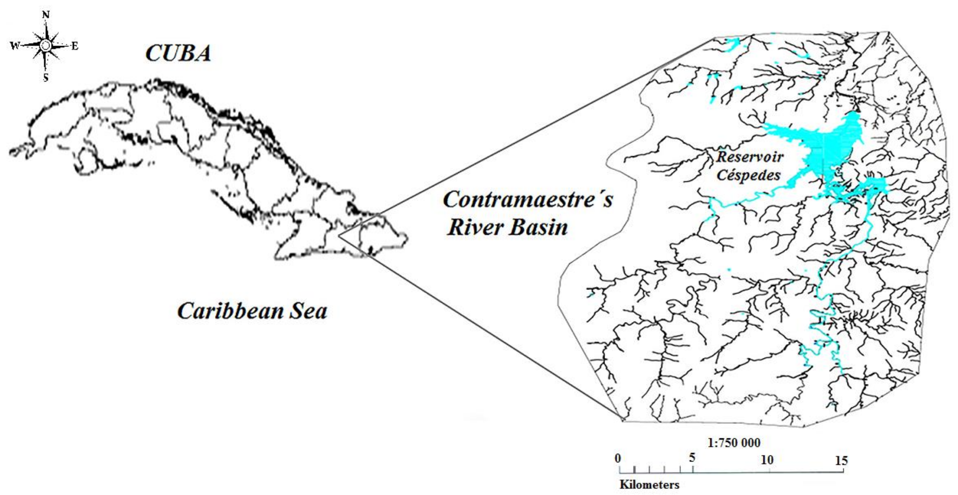
The case study considered in this article is the Carlos Manuel de Céspedes reservoir in the province of Santiago de Cuba, Cuba. The reservoir is located in the Contramaestre River basin at the coordinates corresponding to latitude 180.5° N and longitude 562.7° E, as shown in
Figure 1. The river has a length of 96 km, and its tributary basin has an approximate area of 440.6 km
2. According to the studies carried out by the Delegación Provincial de Recursos Hidráulicos of Santiago de Cuba province, the average annual runoff to Contramaestre River basin has been estimated at 238 Mm
3, of these, 152 Mm
3 (63.86%) occur in the wet season (May–October), and the remaining 86 Mm
3 (36.32%) occur in the dry season (November–April). The average annual rainfall in the basin is 1616 mm. This reservoir has a multi-year or carryover storage refill cycle, and is used in the following order of priority: agricultural irrigation and hydropower. Downstream of the reservoir around 20 agricultural companies are located that annually demand approximately 180 Mm
3.
The reservoir has a total volume of 243 Mm3, an operating storage of 213 Mm3, and the dead storage is 30 hm3. There is a small hydroelectric power station (PCHE) with only one operational turbine, which has an installed capacity of 1500 kW. The turbine requires a minimum operating head of 7.70 m; which is guaranteed because the difference between the dead storage head and the turbine axis is 8 m. The activity of agricultural irrigation is carried out through direct intake from the Contramaestre River. Currently, the reservoir is operated through considering an operational rule that was obtained with a simulation model. The current operating rule establishes that during real-time operation, if the volume of the reservoir is within two guide curves, the save yield can be held. However, this rule does not consider the multipurpose use of the reservoir and the energy production.
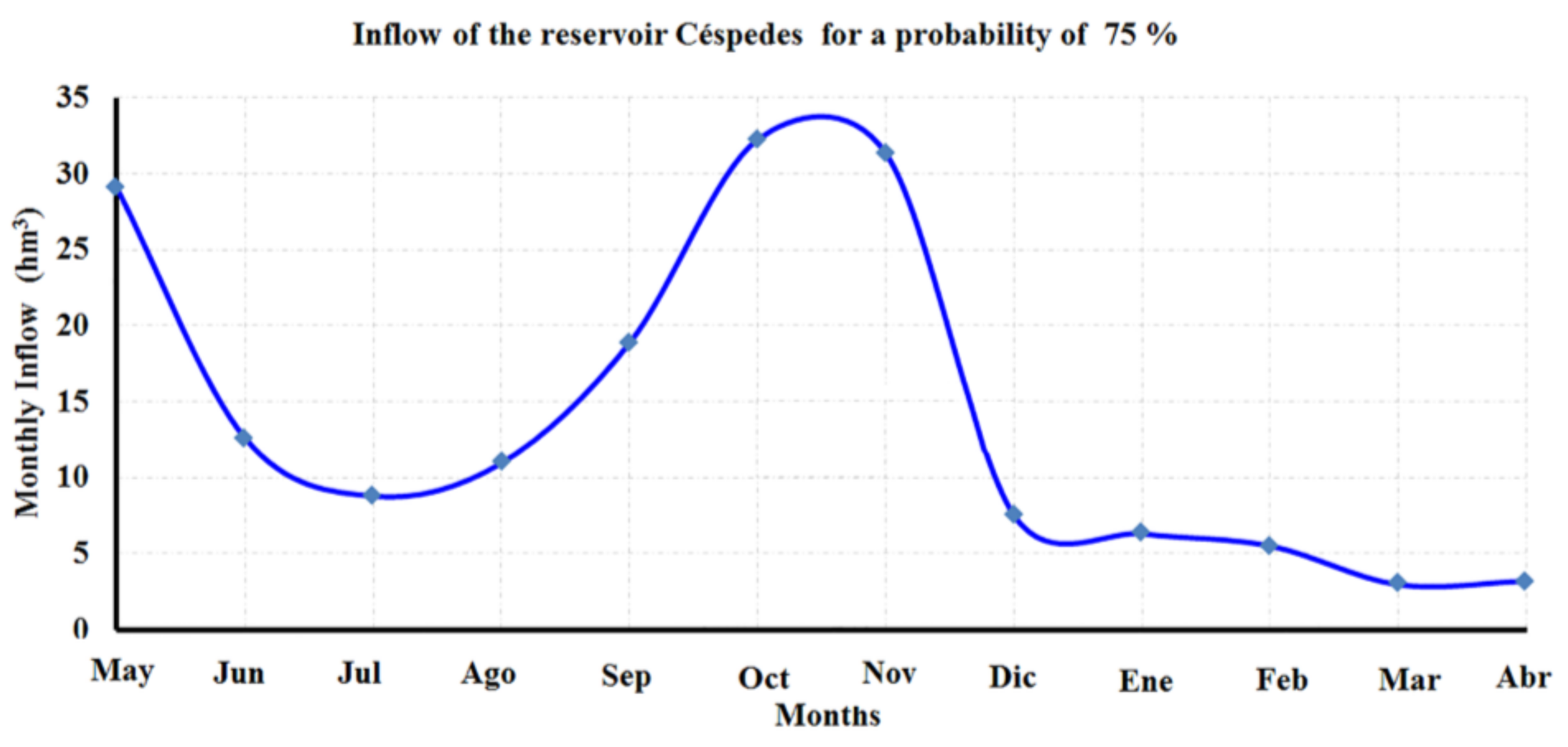
In the present study, a monthly time scale was selected with a total time period of 12 months. Besides, the hydrological cycle begins in May and ends in April. The monthly inflow shown in
Figure 2 corresponds to a probability of 75%, whose mean annual inflow is 169 Mm
3, and the coefficient of variation (
Cv) is 0.55. By using an inflow of this probability, a conservative scenario is applied because it refers to a medium—dry hydrological year. The maximum discharge of the Céspedes reservoir is 5 m
3/s, and the reliability is 75%. It is common to use this reliability when the main user is irrigation.
The unitary deficit cost of the user is set in 1.0 $/Mm3. The annual water demand of 180 hm3 for all of the users (20 agricultural companies) has been distributed uniformly at a constant rate of 15.0 Mm3/month. The fraction of the user’s water demand that is accepted as a deficit has been estimated at 20%, which means that the maximum monthly deficit of all the users is 3.0 Mm3. This value guarantees a volumetric reliability of 80%. The value of the energy tariff is 0.27 $/kW-h. The maximum benefit of the hydroelectric power station has been estimated as 291,600.00 $/month. This value considers that the turbine works at maximum power throughout the month.
A conventional single-objective optimization problem is stated as the problem of finding the point, in a space of decision variables, in which an objective function reaches its minimum value. The optimization problem described previously has two objective functions with a clear conflict between them. For solving this conflict, the constraint-ε method has been adopted; in this way, the multiobjective problem is transformed into a mono-objective problem. In this sense, the main objective function is set to minimize the cost of the annual water deficit in the users, and the objective function that maximizes the annual benefit for the generation of the electricity energy becomes a constraint of the model. The monthly upper limit of this second objective function is
$291,600.00, and the lower bound is set to zero. The optimization technique used in this problem is the genetic algorithms (GA) technique, which is implemented in the mathematical assistant MATLAB 6.0 with the function (
ga). For running the model, 500 generations individuals are set for a population of 200, with crossing and mutation factors of 0.8 and 0.2, respectively.
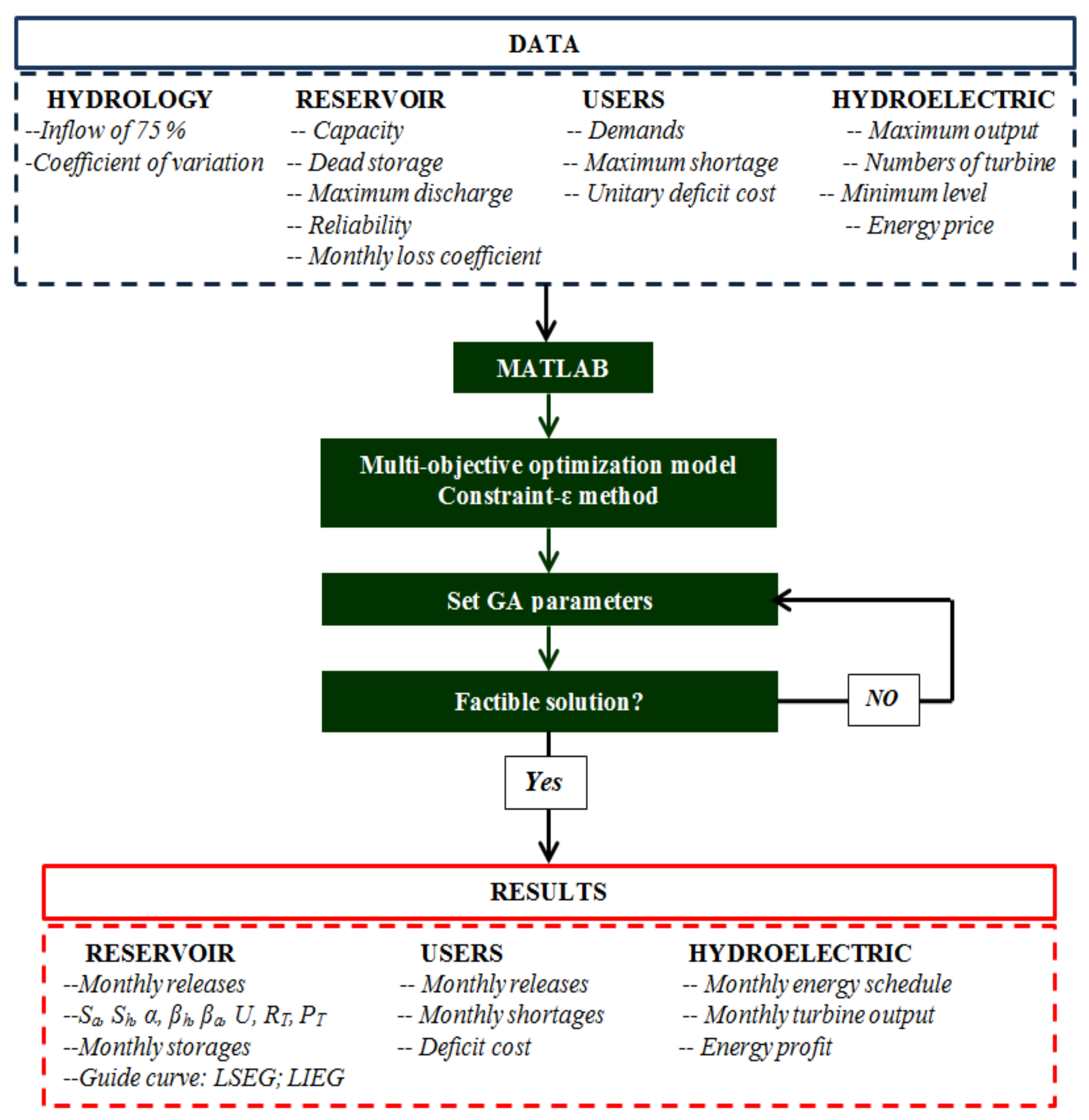
Figure 3 shows the three basic steps for the application of the optimization mathematical model in a functional diagram.
The optimization problem has 28 decision variables due to the 12 monthly releases of the reservoir, the 13 monthly storages for making the guide curve, and the variables α, Sa, and Sh of the Kritsky and Menkel method.
3. Results and Discussion
As previously stated, the first MATLAB execution of the model is made considering parameter λ = 1. The execution of the model shows a good convergence of the GA algorithms; it reaches a good solution, and all of the constraints are fulfilled. The objective function has a value of $22.50, which represents the cost of the annual water deficit to the users. The maximum constraint violation of the model is 1.5 × 10⁻⁸. The model run lasted 35 min in a Dual Core PC with 4 GB of RAM.
Table 1 shows the key parameters for reservoir management. As was previously stated, the degree of reservoir regulation (
α) is a decision variable of the model with a lower and upper bound. The lower bound is 0, and the upper bound is the ratio
U/
Wm. The GA algorithm decides the value of this variable. The reservoir has a high value of degree of regulation (
α), which is due to a strong multi-year o carryover storage behavior that is also reflected in the values of
βh and
Sh. It could be caused by the high value of the parameters
Cv and
α. Equation (12) shows that these parameters have a strong relationship with
βh. On the other hand, once the algorithm determines the value of the variable (
α), the model uses Equations (10) and (12), and calculates the value of the variables (
βa) and (
βh). The high value of
Cv may be an alert of changes in the inflow pattern of the Contramaestre River due to a climate change. This statement should be demonstrated, but it is still a possibility.
The annual net release is 157.5 Mm3; this value could be interpreted as the safe yield of the reservoir for a given inflow time series. The annual water loss is 11.5 Mm3, and the annual gross release is 169 Mm3. The value of the annual gross release confirms the quality in the execution of the model, because it is equal to the annual inflow for a probability of 75%, thus implying that the releases of the reservoir are governed by the inflow.
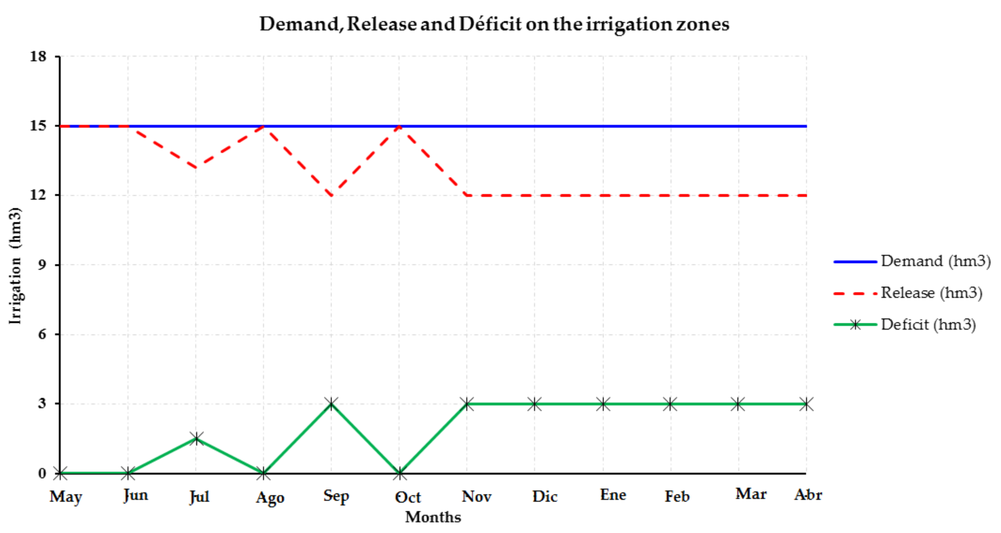
Figure 4 shows the monthly distribution of the demand, releases, and deficits of the irrigation. It is remarkable that in May, June, August, and Oct, the solution proposed by the model satisfies 100% of the demand, and there are no deficits. Those months belong to the wet season, and there is more available, while in the remaining months, the model distributes monthly deficits almost equally. This result is due to the constraint of Equation (37), which forces the algorithm to handle the maximum allowable water deficit. The GA algorithm proposed a good solution, because it is better to have many months with a low deficit than a few months with catastrophic deficits. The volumetric reliability of the users, which is the relationship between the annual net release and the annual water demand, has a value of 87.5%, and is a very good result for these users. With the proposed operation plan, the users will have a deficit of 22.5 Mm
3, which the reservoir will not be able to satisfy.
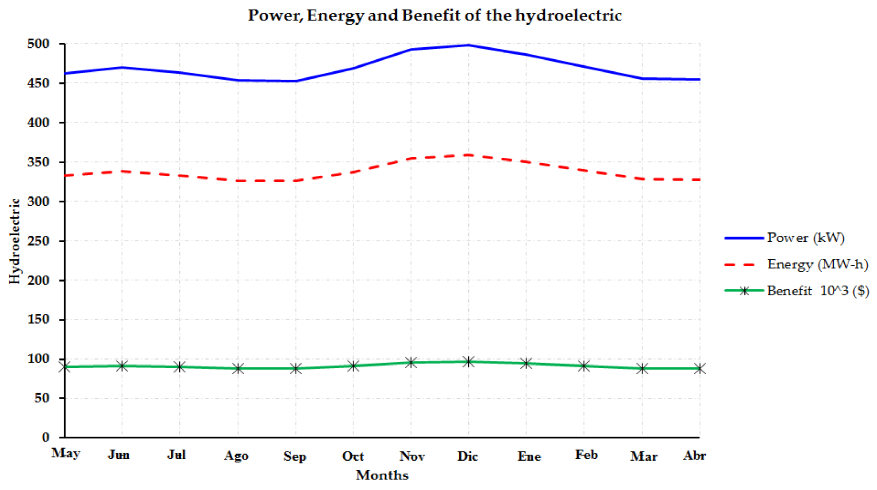
Figure 5 shows the result for the operation of the hydroelectric plant. The chronogram establishes the monthly distribution of the energy to be generated, the monthly average power of the turbine, and the expected benefits. The hydroelectric plant can generate annually 4053.6 × 10
3 kW-h of energy, with a total benefit of
$1094.6 × 10
3. This operational schedule is very useful for the Delegación Provincial de Recursos Hidráulicos of the Santiago de Cuba province. First, the installed turbine in the reservoir is too big for this system, because the maximum power proposed by the model is 498 kW, and the installed power is 1500 kW. So, this turbine can only work with about one third of its power.
With the results obtained in the first execution of the model and through Equation (39), it is possible to determine the parameter λmin = 0.40. This is the minimum fraction of the operating reservoir storage capacity for making the second execution of the model. After running the model with λmin, it is possible to get the storages, levels, and releases corresponding to the guide curve that represents the Lower Line of Safe Release (LLSR).
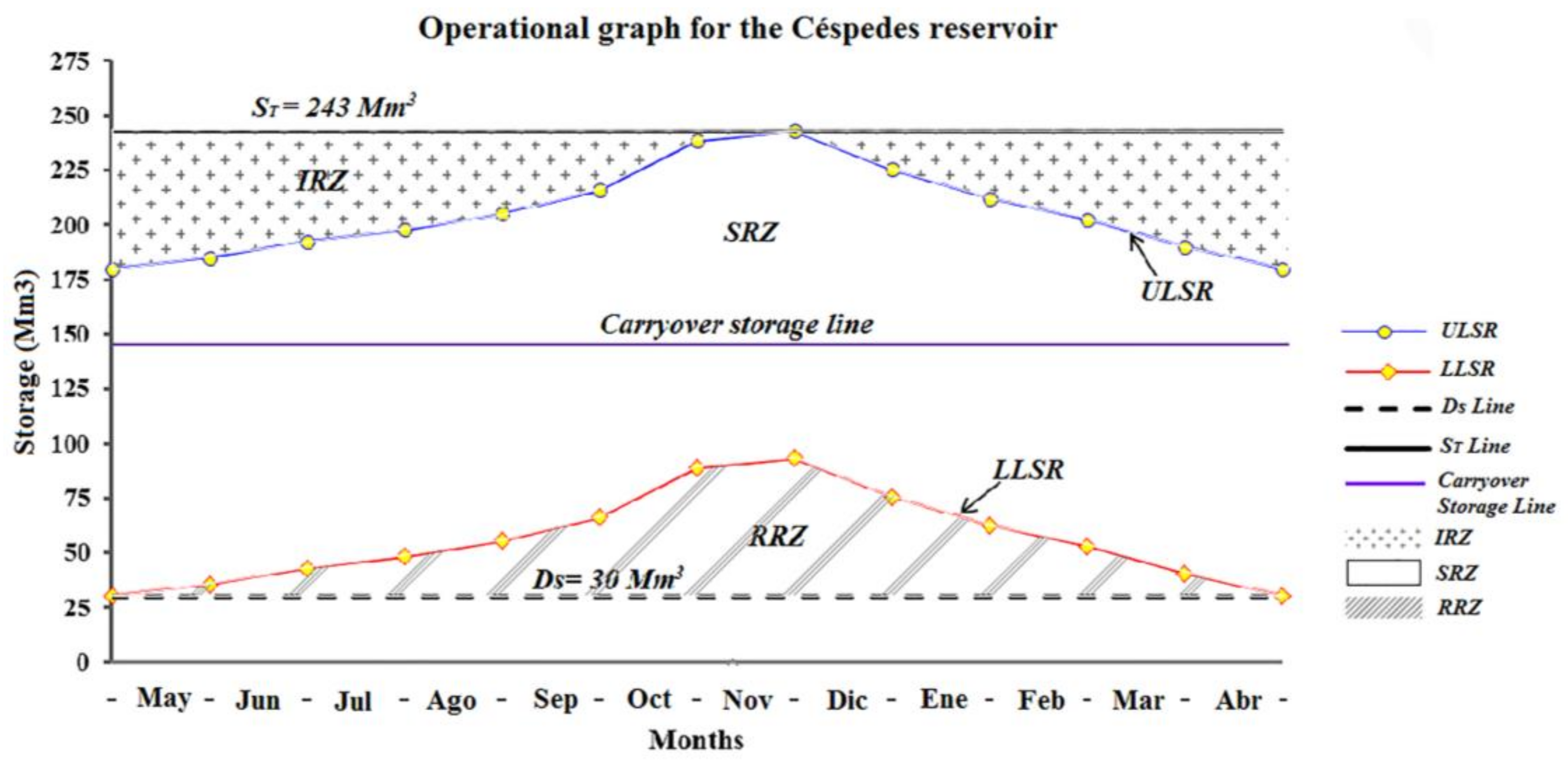
The (
ULSR) and (
LLSR) obtained are very useful for making the operational graph of the reservoir, and establishing the ideal storages that ought to be maintained in each time period in order to archive the annual net release. This two guide curves must be placed within the same graph and add straight lines with the dead storage (
Ds), the total storage (
ST), and a line to represent the multi-year or carryover storage component of the reservoir. This graph is shown in
Figure 6, and plays a fundamental role in the long-term reservoir operation. The operational graph implicitly conceives the operating rules for real-time reservoir operation based on the stage (storage) and the time (months) of the year. The operational graph of the reservoir is divided into three main zones delimited by the (
ULSR) and the (
LLSR). The zones can be classified into the:
Zone of Increased Release (
IRZ), the
Zone of Safe Release (
SRZ), and the
Zone of Reduced Release (
RRZ). The (
IRZ) is located between the line of the
Total Storage (
ST) and the curve of the (
ULSR); the (
SRZ) is located between the (
ULSR) and the (
LLSR), and the (
RRZ) is located between the (
LLSR) and the dead storage (
Ds).
The zones establish the operating rules for the real-time reservoir operation, and the guide curves and lines are the triggers for the beginning of actions in order to improve the management of the reservoir.
Rule 1: If the storage of the reservoir is placed in the (IRZ) zone, then the monthly release can be increased beyond the monthly target release until the storage of the reservoir goes below the ULSR line. This increase does not affect the operational scheme proposed for the reservoir, because it would be spilled water otherwise. Under this scenario, the irrigation demand could be fully satisfied, and the energy generated might be increased.
Rule 2: If the storage of the reservoir is placed in the (SRZ) zone, then the monthly target release can be achieved, and the monthly target energy generated can be normally satisfied.
Rule 3: If the storage of the reservoir is placed in the (RRZ) zone, then the monthly target release should be reduced in order to make the reservoir storage go back to the (SRZ) zone and avoid a catastrophic failure in the supply of the reservoir.
The operational graph includes the carryover storage line within the (SRZ) zone. Through this line, it is possible to identify when the carryover storage is used in the reservoir operation. While the reservoir storage is above the line, the within-year storage component is used; otherwise, the multi-year or carryover storage component of the reservoir is being used. This line also gives a hint to the reservoir operator, because if the storage is below this line, then the target release might be reduced in order to preserve the water for delivering in the future.
The proposed mathematical optimization model appropriately reflects the reservoir operation behavior. The amount of constraints included into the model represent the physical, operational, and hydrological characteristics of the reservoir and the hydroelectric power plant. Furthermore, Kritsky and Menkel’s method determines the carryover storage magnitude. The response of the model is quite sensible to the inflow time series, as previously stated, so the mean annual inflow (Wm) and the annual inflow for a given probability (Wg) should be selected carefully for the modeler. The value of the degree of regulation (α )is the other sensible variable that plays a key role regarding the values of the variables βh, Sh, βa, and Sa. The main drawback of this study is that the model uses a one-year inflow time series that does not allow analyzing a result that considers too many hydrological scenarios. The constraint-ε method is very simple in practice, but provides only one solution for solving the model. Consequently, the drawbacks of this study are exceeded considerably by the applicability of the result. First, the proposed model is able to define the optimal operating policy of the reservoir, because it provides the monthly amount of water that the reservoir should release in each time period in order to minimize the water deficit on the user. This automatically provides the guide curves and operating rules for long-term reservoir operation, and determines the magnitude of the carryover storage. This content is very original and important, because it is a volume that ought to be held on the reservoir for future uses. Second, the monthly energy generation schedule proposed by the model is the goal for the hydroelectric real-time operation, and provides a guide for the reservoir operators for reaching the proposed benefit. Third, the operation graph of the Céspedes reservoir provides an effective tool for reservoir management during real-time operation. Consequently, it provides a mechanism for controlling the releases and the storage of the reservoir according to the time of the year. Another advantage of this graph is that it includes guide curves and operating rules that are used as a trigger indicator to start different measures or actions in the reservoir. Reservoir operators commonly use these during the real-time operation.
Climate change is a challenge for reservoir operation. In the future, the hydrological time series could suffer a chaotic change in the values of the mean inflow and the coefficients of variation. This effect might cause the reservoir that currently has an intra-annual filling–emptying cycle in the future to have an interannual filling–emptying cycle. The proposed model is suitable and versatile, because it could be applied in a reservoir with and without carryover storage. Consequently, it could be possible to identify the reservoir or reservoirs that are changing their filling–emptying cycles due to the climate change effect.
4. Conclusions
The present paper shows a new multiobjective optimization modeling approach for multipurpose single reservoir operation. The proposal model is used to determine the optimal operation policy in reservoirs with carryover storage behavior. The most interesting aspect of the paper is the proposed mathematical model that implicitly conceives Kritsky and Menkel’s method for designing the reservoir operating storage capacity, and it is modified for the reservoir’s operational stage. Through the use of the model, it is possible to get the carryover storage magnitude of the reservoir, as well as its monthly release schedule, the guide curves, operating rules, and the key parameters for the management of the reservoir.
The mathematical model is implemented through the mathematical assistant MATLAB with a multiobjective modeling approach. To run the optimization model, the GA is used; once again, it is demonstrated that this optimization technique is suitable and provides good results regarding problems in water resources management. For solving the multiobjective optimization problem, the constraint-ε method is used. In this sense, the main objective function is to minimize the cost of the annual water deficit for the users, and the secondary objective function is to maximize the annual benefit of the electrical energy generated. This second objective function was implemented as a constraint of the mathematical optimization problem.
The proposed model is applied in order to obtain an operational scheme to the Carlos Manuel de Céspedes reservoir in the Santiago de Cuba province. As practical results, the monthly target release of the users, the energy generation schedule, key parameters for the management of the reservoir, the carryover storage magnitude, the operational graph, the operating rules, and the guide curves for long-term operation are obtained. The proposed operational scheme and the results obtained from the execution of the model contribute to improving the management of the water resource in this reservoir, because it can be applied to both the planning and real-time operational stages.


 and
and 


