Abstract
In order to mitigate environmental and ecological impacts resulting from groundwater overexploitation, we developed a multiple-iterated dual control model consisting of four modules for groundwater exploitation and water level. First, a water resources allocation model integrating calculation module of groundwater allowable withdrawal was built to predict future groundwater recharge and discharge. Then, the results were input into groundwater numerical model to simulate water levels. Groundwater exploitation was continuously optimized using the critical groundwater level as the feedback, and a groundwater multiple-iterated technique was applied to the feedback process. The proposed model was successfully applied to a typical region in Shenyang in northeast China. Results showed the groundwater numerical model was verified in simulating water levels, with a mean absolute error of 0.44 m, an average relative error of 1.33%, and a root-mean-square error of 0.46 m. The groundwater exploitation reduced from 290.33 million m3 to 116.76 million m3 and the average water level recovered from 34.27 m to 34.72 m in planning year. Finally, we proposed the strategies for water resources management in which the water levels should be controlled within the critical groundwater level. The developed model provides a promising approach for water resources allocation and sustainable groundwater management, especially for those regions with overexploited groundwater.
1. Introduction
Groundwater is being overexploited in many regions of the world due to increasing demand for water resources brought about by rapid economic development and population growth [1,2]. It causes a variety of problems such as drawdown of groundwater levels, drying up of aquifers [3], increase in the groundwater cones of depression [4], and land subsidence [5]. Intensive irrigation can lead to the development of salinity problems, and the extraordinary rise of piezometric surface in aquifers may induce groundwater inundation [6], resulting in several damage processes such as building foundation destabilization, groundwater infiltration and pollutant remobilization [7]. Thus, considerable attempts have been made to control groundwater exploitation and water level [8]. In China, the State Council stipulated the implementation of controlled groundwater exploitation in those groundwater overexploited regions [9].
Many models have been developed to optimize groundwater exploitation and address the impact of groundwater overexploitation. Commonly used methods for groundwater simulation include finite difference method, finite element method, boundary element method and finite volume method. Mehl and Hill [10] proposed a new method of local grid refinement for two-dimensional block-centered finite-difference meshes in the context of steady-state groundwater flow modeling. Wang et al. [11] proposed a groundwater flow domain decomposition model coupling the boundary and finite element methods. However, Anderson and Woessner [12] pointed out the accuracy and reliability of groundwater numerical models depended critically not only on the simulation method but also on the properly generalized conceptual hydrogeological model. Recent decades have also witnessed significant progress in the development of groundwater simulation software based on the conceptual hydrogeological model, such as the groundwater simulation modeling system (GMS) [13], modular three-dimensional finite difference groundwater flow model (MODFLOW) [14], finite element groundwater flow modeling software (FEMWATER) [15], and finite element subsurface flow system (FEFLOW) [16]. These models have achieved remarkable success in investigating groundwater levels [17], groundwater mass balance [18], salt transport in coastal aquifers [19,20], groundwater quantity balance [21], impact of predicted climate changes on groundwater flow systems [22], sustainable groundwater management [23,24], and groundwater irrigation [25]. However, given the “natural-artificial” dualistic characteristics of the water cycle system [26], water resources allocation can have significant impacts on the groundwater recharge and discharge, resulting in significant changes in groundwater exploitation and consequently changes in water level. Thus, groundwater numerical models coupled with optimal allocation of water resources can provide a more effective way to simulate groundwater in complex regions.
Artificial fish swarm algorithm [27], multi-objective optimization [28,29,30], interval-parameter multi-stage stochastic programming model [31], ant colony optimization [32], support vector machines and genetic algorithms [33] have often been used in coupling groundwater-surface water models. These models make it possible for the dynamic allocation of water resources in different regions in reference year [34]. Lu et al. [35] showed that the coupling of water resources allocation models and groundwater numerical models reduced the allowable and overexploitable quantity of groundwater for quantifying the groundwater allowable withdrawal accurately in planning years.
Groundwater level can be indicative of groundwater quantity and underflow, and thus, it is an important index in groundwater management. Knowledge of spatial and temporal changes in groundwater levels following the optimal allocation of water resources is essential to better understand the stability of groundwater environment [36]. Jang et al. [37] quantified the recovery of groundwater levels in townships when groundwater for drinking and agricultural demands was replaced by surface water based on the groundwater-surface water coupled model. In order to more accurately control the groundwater level in the canal-well irrigation district, Su et al. [38] simulated the spatiotemporal groundwater depth in planning year using the optimal allocation model of water resources coupled with the groundwater numerical model. Stefania et al. [39] modeled groundwater/surface-water interactions in an Alpine valley (the Aosta Plain, NW Italy) to investigate the effects of groundwater abstraction on surface-water resources.
In summery, previous studies have focused mainly on the modification of numerical modeling and groundwater exploitation calculation [40,41,42], while changes in future groundwater levels were seldom considered. Thus, this study aims to consider changes in future groundwater levels, as well as changes in groundwater exploitation in water resources allocation. A water resources allocation model is constructed to predict future groundwater recharge and discharge, and the results are input into the groundwater numerical model to forecast changes in water levels. The established groundwater numerical model will be adopted to feedback the allocation results. Groundwater exploitation and water level are quantified by using multiple-iterated technique to achieve dual control. Also, groundwater allowable withdrawal and critical groundwater level are used as feedback factors to optimize the model. However, changes of groundwater exploitation and water level will affect the natural equilibrium state of groundwater system and environment. Thus, the proposed multiple-iterated dual control model makes contributions to hydrogeology.
The groundwater over-exploited region in Shenyang of northeast China is selected as the study area. The main purposes of this study are to (1) evaluate the performance of groundwater numerical model in simulating water level and calculate the critical groundwater level; (2) simulate spatial and temporal changes in groundwater levels and propose a scheme for sustainable groundwater management; (3) investigate spatial and temporal changes in groundwater levels under different precipitation conditions in the future; and (4) evaluate the performance of the multiple-iterated dual control model in controlling groundwater exploitation and water level.
2. Study Area and Methods
2.1. Study Area
The groundwater over-exploited region in Shenyang, the capital city of Liaoning Province in northeastern China, is selected as the study area (geographical coordinates, 41°11′51″–43°02′13″ N and 122°25′09″–123°48′24″ E, see Figure 1). It is a plain area administratively divided into Urban District, Shenbei New District, Sujiatun District, Hunnan New District, Yuhong District and Development Zone with a total area of 2318 km2. There are a total of 36 municipal water sources in the study area, as shown in Figure 1, which are the main source of groundwater.

Figure 1.
Geographical location of the study area and distribution of municipal water sources.
Figure 2a shows changes in groundwater exploitation and average water level in the study area over the period 2004–2013. Clearly, groundwater exploitation increases from 2005 to 2007 and then decreases from 2007 to 2009. However, it is noted that groundwater exploitation increases again to a maximum of 403.01 million m3 in 2010. Groundwater level decreases to a minimum of 31.07 m in 2010, after which it increases continuously. Two water transfer projects (Dahuofang and Liaoxibei) were constructed in 2011, and the government of Liaoning Province had taken measures to close many groundwater sources to stop decline of water level due to groundwater overexploitation. Now, the transferred water are used instead of groundwater since 2012.
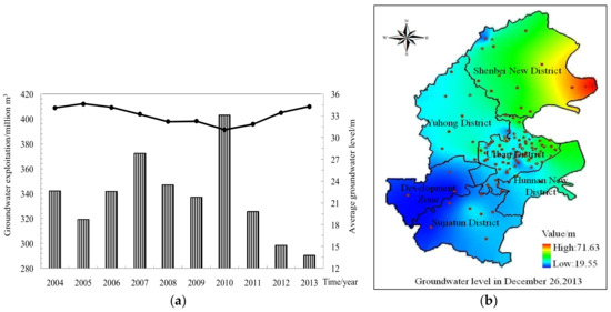
Figure 2.
(a) Changes in groundwater exploitation and average water level in 2004–2013; (b) Spatial distribution of groundwater level and location of monitoring wells in 2013.
Figure 2b shows spatial distribution of groundwater level and location of monitoring wells in 2013. The spatial distribution of groundwater level is plotted based on the monitored groundwater level by the 114 monitoring wells. Due to the influence of topography, groundwater level is generally high in the northeast but low in the southwest. It is important to note that despite the decrease in groundwater exploitation quantity, groundwater overexploitation remains a serious problem in 2013, resulting in the formation of three cones of depression with a maximum groundwater depth of 20.77 m.
2.2. Research Framework and Simulation Model
Figure 3 shows the multiple-iterated dual control model for groundwater exploitation and water level, which consists of the following four modules, including optimal allocation module of water resources, groundwater allowable withdrawal calculation module, groundwater simulation module, and groundwater level control module. This study focuses mainly on the dual control for groundwater exploitation and water level and the interactions of the four modules, so the procedures for development of water resources allocation model can be referred to Zhou [43]. The details are provided in the Appendix A.
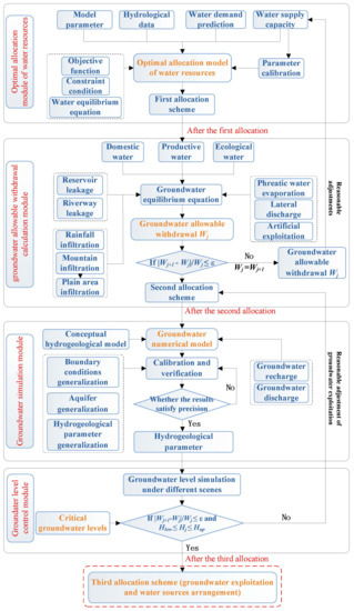
Figure 3.
Study framework for multiple-iterated dual control model for groundwater exploitation and water level.
The model focuses on the coupling of water resources allocation and groundwater numerical simulation. The surface water supply and groundwater exploitation are coupled in the water resources allocation model to calculate field infiltration and well irrigation regression recharge of the groundwater numerical model. Water supply, demand and deficit are analyzed by different water demand schemes, and the rational allocation of water resources is put forward. The future groundwater level can be predicted by data extraction and interaction, and dual control for groundwater exploitation and water level can be achieved based on groundwater allowable withdrawal and critical groundwater level.
2.2.1. Optimal Allocation Module of Water Resources
The optimal allocation model of water resources consists of a number of objective functions, constraints and water balance equations. In the model long-time series hydrological and economic data and ecological water requirements in different years serve as the inputs. The calculation unit is based on the geographical locations of water resources and administrative regions. The constraints are the water balance constraints, and the objective is to maximize the net benefit of water supply and minimize water loss. The model is solved by the mathematical planning. In this study, the General Algebraic Modeling System (GAMS 2.5) [44] is used to establish and solve the model.
(1) Objective function
The objective is to maximize the net benefit, minimize water loss, and ensure the precedence of water sources for water supply, as described in Equation (1).
where is the vector composed of decision variables; S is the feasible set of decision variables composed of different constraints; and is the objective for the development of society and economy, ecological environment and water resources.
(2) Constraints and water balance equations
The constraints and water balance equations are described in Wei et al. [45]. The groundwater supply constraints and balance equations in the calculation unit are shown in Equation (2).
where XZGC, XZGI, XZGE, XZGA, and XZGR are the groundwater supply for urban domestic use, industrial use, urban ecological use, agricultural use, and rural domestic use (million m3), respectively; PZGTU is the exploitable coefficient of groundwater in the calculation period; PZGW is the annual groundwater availability (million m3); tm is the calculation period; and J is the calculation unit.
In general, the main data of this module include the predicted water demand, water supply of municipal water sources, and model parameter. The supplemental materials and the first water allocation scheme are listed in Table A1, Table A2, Table A3, Table A4, Table A5, Table A6, Table A7, Table A8, Table A9 and Table A10.
2.2.2. Groundwater Allowable Withdrawal Calculation Module
Groundwater allowable withdrawal is used to judge whether groundwater in a given region is exploited reasonably. It is used as a feedback of the water resources allocation model. In the study area, the shallow groundwater is the main water source and it is phreatic water. The allowable withdrawal of shallow groundwater is defined as the maximum quantity of groundwater that can be extracted from the aquifer without causing environmental and geologic impacts on the premise of economic and technical feasibility. It can be calculated by mining coefficient method based on groundwater balance method [46] (Equation (3)).
where W is the groundwater allowable withdrawal (million m3); Wr is the quantity of groundwater recharged by precipitation infiltration, mountain and plain area infiltration, reservoir and riverway leakage, and other recharges (million m3); We is the discharge of groundwater resulting from lateral discharge, artificial exploitation, phreatic water evaporation, and other discharges (million m3); ΔS is the changes in groundwater level (m); µ is the specific yield of phreatic water aquifer; F is the area of equilibrium region (km2); Δt is the time span of equilibrium period; ρ is the exploitable coefficient, which is related to the long-term series groundwater data, aquifer type, and mining conditions. The calculation of ρ is described in our previous study, and the iterative calculation of groundwater allowable withdrawal is listed in Table A11.
2.2.3. Groundwater Simulation Module
GMS 7.1 consisting of several modules such as MODFLOW, FEMWATER, and MODPATH is used in this study to develop the groundwater simulation model, and the equations are composed of fundamental differential equations describing the three-dimensional unsteady groundwater flow in porous media, boundary conditions, and initial constraints (Equation (4)). The MODFLOW module is used for groundwater simulation in this study.
where K is the aquifer permeability coefficient; Kx, Ky, and Kz are the component of the permeability coefficient along the x, y and z directions, respectively (m/d); W is the source term per unit volume (m3/d); μ is the specific yield of the phreatic water aquifer; H is the groundwater level (m); H0 is the initial water level (m); B is the aquifer floor elevation (m); q is the discharge per unit width under the second type boundary conditions (m3/d/m); x, y and z are the coordinates (m); n is the inner normal on the boundary; and Γ1 and Γ2 are the first and second type boundary, respectively.
The accuracy of groundwater simulation is determined based on the average relative error (ARE), mean absolute error (MAE), and root-mean-square error (RMSE) (Equations (5)–(7)).
where Hi and Hi′ are the observed and calculated groundwater level (m), respectively, and n is the length of sample series.
2.2.4. Groundwater Level Control Module
A critical groundwater level Hc is set in this study in order to prevent potential environmental and geological impacts resulting from too high or too low groundwater levels, and it is established according to the function of different groundwater systems in different areas. The upper and lower limits of the critical groundwater level (Hup and Hlow) are determined for each region to control groundwater exploitation and water level more reasonably (Equations (8) and (9)).
where H1 is the critical groundwater level for frost heaving and boiling (m), Hfrost is the frost line (m), H2 is the critical groundwater level for soil salinization (m), H3 is the anti-floating design water level for underground orbit traffic (subway) (m), H4 is the waterproof design water level for underground structures (m), Huph is the historical maximum water level (m), Hupl is the maximum water level in the recent 3–5 years (m), M is the aquifer thickness (m), and h is the ground elevation (m), respectively.
The average critical groundwater level is calculated from groundwater levels of all monitoring wells by the Thiessen Polygons method described in Equation (10) [47].
where and A are the average critical groundwater level (m) and area (km2) for different regions, respectively; ai is the area of the ith calculation unit of the ith Thiessen polygon, i = 1, 2, …, n (km2); Hci is the critical groundwater level of the ith calculation unit of the ith Thiessen polygon, i = 1, 2, …, n (m); and n is the number of Thiessen polygons.
2.3. Multiple Iteration Processes
The multiple-iterated dual control model is derived from the coupling of the optimal allocation model of water resources and the groundwater numerical model:
Step 1: The topological and recharge-discharge relations among different water systems, water conservancy projects, and water users in reference year are analyzed. The objective functions and constraints are determined, and the optimal allocation model of water resources is established for the calculation of water demand-supply balance in planning year, which is referred to as the “first allocation scheme” in this study.
Step 2: The results obtained from the first allocation scheme are substituted into Equation (3) to calculate the groundwater allowable withdrawal Wj (where j is the number of iterations, j = 0, 1, 2, …, n). If |Wj+1 − Wj|/Wj ≤ ρ (ρ = 0.02), go to Step 3; otherwise let j = j + 1 and return to Step 1. This process is repeated until satisfactory results are obtained, which is referred to as the “second allocation scheme” in this study.
Step 3: The aquifer, boundary conditions, and hydrogeological parameters in the study area are generalized, and the conceptual hydrogeological model and groundwater numerical model are established. Subsequently, groundwater levels are calibrated and verified, and hydrogeological parameters are determined.
Step 4: The results obtained from the second allocation scheme are input into the verified groundwater numerical model to simulate changes in groundwater levels Hj (where j is the number of iterations, j = 1, 2, …, n). If Hlow ≤ Hj ≤ Hup and |Wj+1 − Wj|/Wj ≤ ρ, stop calculation; otherwise, adjust groundwater exploitation Qj and optimize water resources allocation again until the following three requirements are met: (1) the total groundwater supply is lower than groundwater allowable withdrawal and the total water consumption is lower than that mandated by government regulations, (2) water supply-demand balance and groundwater recharge-discharge balance are realized; and (3) the water deficit ratio of each unit is no more than 5%. This scheme is referred to as the “third allocation scheme” in this study.
2.4. Data Collection
The input data of the optimal allocation model of water resources include corrected monthly precipitation and runoff in 1956–2013, river flow data, groundwater recharge in 1980–2013, and social and economic data in water demand. The input data of the groundwater numerical model include water levels of monitoring wells, groundwater exploitation of municipal water sources, and groundwater recharge and discharge in 2007–2013. These data are provided by the water management institutes of Shenyang. Main model parameters include river parameters, water supply channel parameters, irrigation water use efficiency parameters, and reservoir parameters, which are determined by field research and expert consultation. Hydrogeological parameters and recharge coefficients of river and field infiltration are calibrated by the model.
3. Results and Discussion
3.1. Establishment and Verification of the Groundwater Simulation Model
In this section, the groundwater simulation model will be described sententiously, and the readers are referred to our previous paper for details [48].
3.1.1. Hydrogeological Conceptual Model
- (1)
- Conceptualization of aquifer: The geological structure of the study area is simple, and the aquifer is single pore phreatic water of Quaternary period. The aquifer thickness ranges from 19 to 140 m, with an average of 66.01 m. Groundwater resources are abundant in the study area. Basically, the grains are finer in the top layer of the aquifer but coarser in the bottom layer. The top layer is composed of coarse, medium, and fine sands, the middle layer is composed of thin clayey soil, and the bottom layer is composed of sand gravel. The 3D geological structure of the study area is shown in Figure A1. The groundwater flow is conceptualized as a 3D unsteady flow according to the Darcy’s law, as the flow field is relatively flat.
- (2)
- Conceptualization of boundary conditions: (a) Lateral boundary conditions: the northern and southern boundaries with rivers are conceptualized as the first water level boundary; the western boundary in which water is exchanged with neighboring regions is conceptualized as the pervious boundary, while the boundaries of other areas are conceptualized as the second flow boundary; (b) Vertical boundary conditions: the top of the phreatic water aquifer is conceptualized as the water exchange boundary, which receives groundwater recharge and discharge, while the aquifer floor is conceptualized as the impervious boundary because it contacts with bedrock.
3.1.2. Discretization and Solution of Numerical Model
The study area is divided into 18,180 grids (200 rows and 200 columns) by MODFLOW module. Each grid has a length of 300 m, a width of 425 m and an area of 0.1275 km2. To reflect the change of groundwater flow during several hydrological years, model calibration is carried out using a series of observed data from 26 April 2007 to 26 April 2013. Model verification is carried out using a series of observed data from 26 April 2013 to 26 September 2013. Calculations are conducted on a monthly basis. There are 72 and 5 stress periods for calibration and validation, respectively.
3.1.3. Calibration and Verification of Groundwater Simulation Model
(1) Calculation of groundwater recharge and discharge
In this study, groundwater is recharged mainly by precipitation infiltration, lateral recharge, reservoir and riverway leakage, field infiltration, and well irrigation regression, and it is discharged mainly by lateral discharge, artificial exploitation, phreatic water evaporation, and riverway discharge. The specific methods of groundwater recharge and discharge can be referred to Ning et al. [49]. Groundwater equilibrium items are used as input to the groundwater numerical model in the form of area recharge intensity. The results are shown in Table A12.
(2) Calibration and verification
The observed data from 26 April 2007 to 26 April 2013 is used for calibration of parameters; while that from 26 April 2013 to 26 September 2013 is used for verification. There are about 114 groundwater monitoring wells over the period 2007–2013, and ten representative wells in the subareas are selected in this study. The results of two representative wells, Yuhong and Railway Machinery School wells located near the Yuhong and Bainiao water sources respectively, are shown in Figure 4. Clearly, there is a good agreement between calculated and observed groundwater levels for both wells over the period 2007–2012. Specifically, the MAE is 0.44 and 0.61 m, the ARE is 2.16% and 1.89%, and the RMSE is 0.48 m and 0.66 m for the Yuhong well in the calibration and verification periods, respectively. The MAE is 0.53 m and 0.36 m, the ARE is 1.98% and 0.99%, and the RMSE is 0.61 m and 0.37 m for the Railway Machinery School well in the calibration and verification periods, respectively.
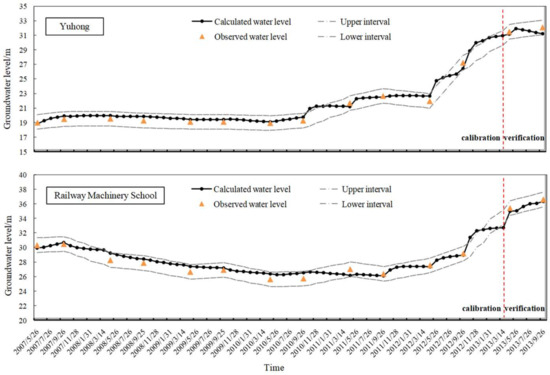
Figure 4.
Annual changes of groundwater levels for Yuhong and Railway Machinery School wells in the calibration and verification periods, respectively.
The spatial distribution of groundwater levels in calibration and verification periods is shown in Figure 5. Due to the influence of concentrated groundwater exploitation in the urban district, the spatial distribution of groundwater levels is very complex with some fitting errors. However, the groundwater levels in the other five districts with less groundwater exploitation are basically regular, and the model fits well.
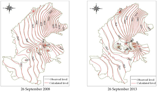
Figure 5.
Spatial distribution of groundwater levels in calibration and verification periods.
Table 1 shows that the MAE of average groundwater levels of the 10 monitoring wells is 0.29 m and 0.44 m, the ARE is 0.98% and 1.33%, and the RMSE is 0.30 m and 0.46 m in calibration and verification periods, respectively, indicating a good agreement between observed and calculated groundwater levels.

Table 1.
The fitting precision of the average groundwater levels of representative monitoring wells in the calibration and verification periods.
To conclude, the MAE, ARE, and RMSE are relatively low, indicating high fitting precision of the model. The established groundwater numerical model can be used for quantitating and forecasting the dynamic future trend of groundwater levels.
3.1.4. Analysis of Parameter Sensitivity and Uncertainty
A total of 68 boreholes and initial values of hydrogeological parameters are determined by field test data and empirical data (Table A13). However, due to the complex heterogeneity of the groundwater system and subjective cognizance, the parameters of groundwater numerical model have uncertainty. Therefore, it is necessary to analyze parameter sensitivity and reduce uncertainty. The permeability coefficient (K) and specific yield (µ) can reflect the permeability of aquifer and declining of groundwater levels, respectively, which are important hydrogeological parameters in groundwater resource evaluation and simulation.
The transforming factor method is used to analyze sensitivity (a parameter as a variable factor and other parameters as invariable factors) [50,51]. The groundwater levels of typical monitoring wells at the end of verification period are output, and changes in groundwater levels are used to reflect parameter sensitivity. The larger change in groundwater levels, the larger effect of parameter on the model. Because the aquifer in the study area is composed of sand and sand gravel, K is 20–150 m/d and µ is 0.1–0.35. After model calibration, K and µ are 50–100 m/d and 0.1–0.2, and thus, K and µ are set to ±20% of initial values. Changes in groundwater levels during parameter variation are shown in Table 2.
Table 2.
The water level changes during parameter variation (units: m).
Table 2 indicates that as K and µ increase, changes in groundwater levels decrease. K has a more significant effect on the model than µ. Therefore, the permeability coefficient is sensitive to the model.
3.2. Critical Groundwater Level
The upper limit of groundwater level in the Urban District with various underground structures and subways is determined primarily based on the anti-floating design water level of subways and the waterproof design water level of underground structures; while that in the other five districts with large well-canal irrigation regions is determined primarily based on the critical groundwater level for soil salinization [52]. According to the hydrogeological conditions of phreatic water aquifer, the maximum drawdown should not exceed 2/3 of aquifer thickness, and the lower limit of groundwater level is the difference between ground elevation and 2/3 of aquifer thickness [53]. The critical groundwater levels for different subareas are calculated by Equations (8)–(10) (Table 3). Table 3 shows that the average upper limit of water levels is 37.72 m, the average lower limit of water levels is −3.18 m, and the average aquifer thickness is 66.01 m. The minimum aquifer thickness is observed in the Urban District, indicating that the aquifer is thin with low water abundance, and thus it is imperative to control groundwater level within the critical groundwater level.
Table 3.
The average critical groundwater level and aquifer thickness of subareas (units: m).
3.3. Optimal Allocation of Water Resources and Groundwater Exploitation Scheme
In this study, the year 2013 is selected as the reference year, while the years 2020 and 2030 are selected as the planning years. Given the rare occurrence of extreme climate events in the history of study area, we focus on the optimal allocation of water resources and changes in groundwater levels in normal years with a precipitation frequency of 50%. The precipitation frequency in 1956–2013 is analyzed and the precipitation in normal years is calculated. The precipitation in 2014–2019, 2020–2029, and 2030–2035 is forecasted by the climate natural variability method [54,55].
3.3.1. Water Supply-Demand Balance
Table 4 and Table 5 show water supply and demand in 2020 and 2030 obtained from the second allocation scheme. The results show that the total water supply in 2020 and 2030 is 2266.26 and 2504.74 million m3, whereas the total water demand is 2273.75 and 2506.23 million m3, respectively, thus indicating a good balance between water supply and demand. According to survey data provided by the water management institute of Shenyang, wastewater treatment plants have been established and operated at the end of 2013. Thus, there is an increase in recycled water supply and transferred water supply but a decrease in groundwater supply in 2020 and 2030, indicating that more surface water is used instead of groundwater, which can contribute to improve groundwater environment. The increased supply of recycled water is from wastewater treatment plants.
Table 4.
Water demand and supply in 2020 (units: million m3).
Table 5.
Water demand and supply in 2030 (units: million m3).
Table 6 shows the calculated groundwater exploitation and groundwater allowable withdrawal after the optimal allocation of water resources. The groundwater exploitation reduces from 290.33 million m3 in 2013 to 87.05 million m3 in 2020 and 109.05 million m3 in 2030, respectively. However, the groundwater exploitation of Hunnan New District remains unchanged in 2020 and 2030 due to extremely high water demand of the national hi-tech industrial development zone. In the first allocation (Table A9 and Table A10), the water deficit of Urban District is 68.93 million m3 in 2030, and therefore the groundwater exploitation in 2030 should be increased to 51.20 million m3, resulting in a decrease of water deficit to 0.07 million m3. However, the overexploitation of Urban District in 2013 is 27.95 million m3, while no overexploitation occurs in other districts, indicating that the controlled measure of groundwater exploitation results in effective mitigation of groundwater overexploitation.
Table 6.
Calculated groundwater exploitation and groundwater allowable withdrawal under the controlled measure of groundwater exploitation (units: million m3).
3.3.2. Spatial and Temporal Changes in Groundwater Levels
The recharge and discharge of groundwater obtained from the second allocation scheme and precipitation in normal years are put into the groundwater numerical model to simulate changes in groundwater levels. We assign 22 stress periods for future prediction from 1 January 2014 to 1 January 2036. Time step is one year. Figure 6 shows that the groundwater levels of water sources (201, Libayan, Songjiang and Beiling) are higher than the upper limit of water level in 2014–2030, and the average groundwater level is increased by 2.52 m. At the beginning of 2034, the groundwater level of Libayan is expected to be 2.1 m higher than the upper limit of water level, whereas that of other water sources is expected to lower than the upper limit of water level. It is also noted that the groundwater levels of all water sources in simulation period are higher than the lower limit of water level. The increase and then decrease in groundwater level coincide well with the decrease and then increase in groundwater exploitation.
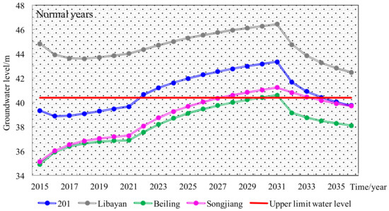
Figure 6.
Temporal changes in groundwater levels of water resources obtained by the second allocation scheme.
Under the second allocation scheme, the groundwater levels decrease from the northeast to the southwest (Figure 7a). Figure 7b shows the spatial distribution of elevation. However, due to controlled groundwater exploitation, the cones of depression observed in 2013 disappear in 2035, and the average groundwater level increases from 34.27 m in 2013 to 34.81 m in 2035. The highest and lowest groundwater level are 73.53 m and 18.32 m, and the average groundwater depth is recovered to 4.92 m. Although the average groundwater level of study area does not exceed the upper limit of water level, there are some water sources with a groundwater level higher than the upper limit of water level, indicating the need to consider the effect of groundwater exploitation on local water sources.
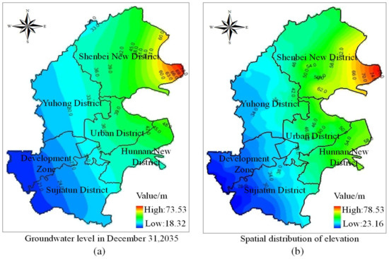
Figure 7.
(a) Spatial distribution of groundwater levels under the second allocation scheme at the end of 2035; (b) Spatial distribution of elevation.
3.3.3. Groundwater Exploitation Schemes and Water Sources Arrangement
In China, for controlling groundwater overexploitation, the government sets a restrictive groundwater exploitation for each city every year. However, we do not know how the groundwater level will change with this restrictive groundwater exploitation and whether this value is reasonable. So we want to search an appropriate groundwater exploitation that does not exceed the restrictive value for water resources optimal allocation. Then put the appropriate value into groundwater numerical model and simulate the groundwater level. If the water level is between the upper and lower limits of water level, the groundwater exploitation is reasonable. The reasonable value is considered as the recommended groundwater exploitation.
Considering that the groundwater level of Libayan is expected to exceed the upper limit of water level at the end of simulation period, it is necessary to calculate the groundwater exploitation of the Urban District in 2030 on the premise of ensuring groundwater recharge-discharge balance in 2020. Finally, groundwater exploitation of Urban District in 2030 is recommended by reasonably adjusting groundwater exploitation. The average groundwater level is 34.72 m and the groundwater levels of all municipal water sources are within critical groundwater level in 2035. Thus, the recommended groundwater exploitation is obtained.
Figure 8 shows the recommended arrangement of municipal water sources at the end of simulation period. There are a total of eleven municipal water sources in the study area, including six water sources in Urban District (20.86, 11.44, 10.04, 9.12, 6.57 and 0.88 million m3 for Xinnanta, Shashan, Libayan, Beiling, 201, and Songjiang, respectively), two water sources in Shenbei New District (12.23 and 2.55 million m3 for Huangjia and Shifosi, respectively), one water source in Yuhong District (17.52 million m3 for Jingsai), one water source in Sujiatun District (7.3 million m3 for Suxi), and one water source in Hunnan New District (18.25 million m3 for Hunnan). The total groundwater exploitation is 116.76 million m3, with a decrease of about 173.57 million m3 compared with that in 2013. According to the “closing scheme of groundwater source implemented by government”, most of groundwater sources are closed and few are reserved. On the one hand, water sources are located close to rivers and allow for the recharge of groundwater from river water. On the other hand, the water levels of some areas have trends that exceed the upper limit. Water sources of these areas need to be reserved.
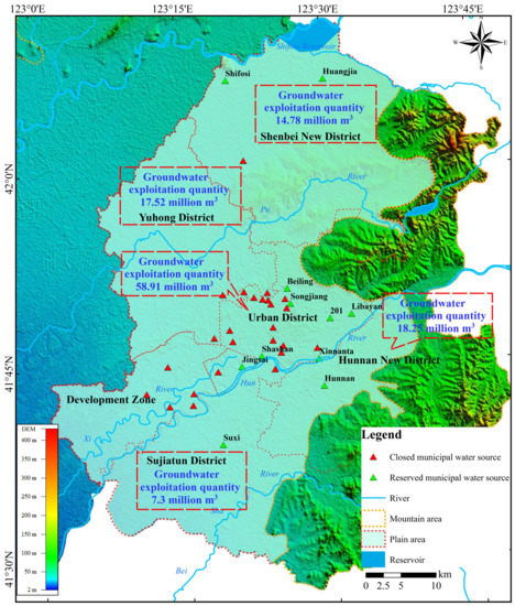
Figure 8.
Recommended arrangement of municipal water sources at the end of simulation period.
3.4. Spatial and Temporal Changes in Groundwater Levels under Different Precipitation Conditions
The groundwater levels obtained by the recommended scheme in wet (precipitation frequency is 25%) and dry (precipitation frequency is 75%) years are shown in Figure 9 and Figure 10. Figure 9 shows the spatial distribution of groundwater levels in wet and dry years, respectively. The average groundwater level increases from 34.27 m in 2013 to 36.63 m in 2035 in wet years and reduces to 31.77 m in dry years, with a change of 2.36 m and −2.50 m, respectively. The average groundwater depth is 2.52 m and 7.93 m in wet and dry years, respectively. The precipitation is higher in wet years, resulting in an increase in surface water supply. Consequently, the precipitation infiltration and groundwater level increase. However, the groundwater level reduces significantly in dry years. Figure 9 indicates that the influence of precipitation and groundwater exploitation on groundwater level is very obvious in the same region.
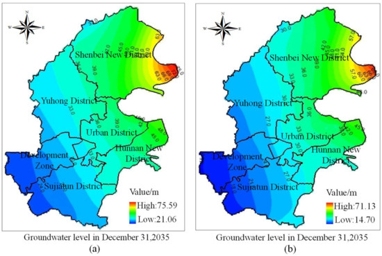
Figure 9.
Spatial distribution of groundwater levels in wet and dry years. (a) Spatial distribution of groundwater levels at the end of 2035 in wet years; (b) Spatial distribution of groundwater levels at the end of 2035 in dry years.
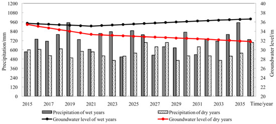
Figure 10.
Temporal changes in groundwater levels in wet and dry years, respectively.
Figure 10 shows temporal changes in groundwater levels in wet and dry years. The groundwater levels in wet years show a decreasing and then increasing trend, whereas that in dry years show a decreasing trend. The differences in groundwater levels between dry and wet years range from 0.27 m to 4.86 m with an average of 0.92 m and 3.33 m in 2015–2020 and 2020–2035, respectively. Changes in precipitation in different hydrologic years can have significant effects on the groundwater level, and the decrease rate of groundwater level is higher than the increase rate. Figure 9 and Figure 10 indicate that precipitation is still a significant factor affecting groundwater level under the recommended scheme of groundwater exploitation. Climate change plays an important role in affecting groundwater level.
3.5. Evaluation of the Multiple-Iterated Dual Control Model
In order to evaluate the performance of the recommended scheme, we compared recommended groundwater exploitation, maximum groundwater exploitation stipulated by government, and average groundwater allowable withdrawal, as shown in Table 7. It shows that the recommended groundwater exploitation is 87.05 and 116.76 million m3 in 2020 and 2030, respectively, which is lower than the maximum groundwater exploitation (259.66 million m3) and average groundwater allowable withdrawal (812.48 million m3). The groundwater exploitation of each subarea is also within the range of maximum groundwater exploitation and average groundwater allowable withdrawal.
Table 7.
Evaluation of the recommended groundwater exploitation (units: million m3).
Table 8 shows that at the end of simulation period, the groundwater levels of all water sources in normal and dry years are within the average critical groundwater level, whereas that of three water sources in Urban District are above the upper limit of water level in wet years. However, the average groundwater level is within the average critical groundwater levels (3.18–37.72 m). Thus, the recommended scheme can satisfy water demand and realize rational utilization of water resources. However, for those water sources with a groundwater level higher than the upper limit in wet years, it is necessary to take appropriate measures to develop groundwater, so that the groundwater level can be kept in the appropriate range, such as constructing water conservation and utilization system and establishing landscape fountains. These methods are suggested measures for realizing this purpose.
Table 8.
Groundwater levels in different hydrologic years and average critical groundwater levels (units: m).
3.6. Discussion of Model Applicability
Groundwater overexploitation has triggered a series of ecological and environmental problems in north China. In 2012, the State Council of China developed a policy to “implement the strictest water resources management system”, which suggested that both total groundwater exploitation and water level should be properly controlled. However, this policy has not been strictly enforced in many regions due to lack of effective management policies and measures. The multiple-iterated dual control model proposed in this study can contribute significantly to reducing groundwater overexploitation in Shenyang, which can also provide important insights into control of groundwater exploitation and water level in other regions. In the study area, the groundwater storage and level have recovered in 2016 [56]. This model has been used to control groundwater depth and realize rational utilization of water resources in other canal-well irrigation regions of China, such as Shanxi [38], and to control groundwater exploitation in Beijing by setting up underground reservoir and allocating irrigation schemes [57]. However, this model is still in the exploratory stage and needs to be further improved to expand its applicability. At present, we attempt to make this model applicable to other groundwater overexploitation areas in China or in the world.
4. Conclusions
In this study, a multiple-iterated dual control model is proposed for short-term and long-term groundwater resources management. This model integrates the optimal allocation model of water resources and the groundwater numerical model, thus making it possible to achieve dual control of groundwater exploitation and water level. It has been successfully applied to the groundwater simulation in Shenyang of Liaoning Province, China. The following conclusions could be drawn:
There is a good agreement between calculated and observed groundwater levels for Yuhong and Railway Machinery School wells over the period 2007–2012, indicating that the groundwater numerical model performs well in simulating groundwater levels with high accuracy.
The optimal allocation of water resources makes it possible for the attainment of water supply–demand balance and groundwater recharge–discharge balance. As a result, the groundwater exploitation reduces from 290.33 million m3 in 2013 to 87.05 million m3 in 2020 and 116.76 million m3 in 2030, respectively.
The controlled exploitation of groundwater results in a disappearance of cones of depression and a rapid recovery of groundwater levels in normal years. The average groundwater level increases from 34.27 m in 2013 to 36.63 m in 2035 in wet years, recovers to 34.72 m in normal years, and reduces to 31.77 m in dry years, respectively. The groundwater exploitation is controlled between the groundwater allowable withdrawal and the maximum groundwater exploitation, and the groundwater levels are controlled within the critical groundwater level.
Water demand predictions of social economy development and ecological environment consider sustainable development in the economy. The optimal allocation model of water resources realizes water supply–demand balance. Regional water resources are rationally allocated in order to achieve better economic and social development. When groundwater is overexploited, it recovers slowly. The multiple-iterated dual control model can be used in overexploitation areas in which surface and transferred water can be used to replace groundwater, and it contributes significantly to economic development, environmental protection, and sustainable groundwater exploitation.
However, there are some limitations in this model. For instance, although future precipitation changes and groundwater exploitation schemes have been considered in this model, some other uncertainties, such as temperature and groundwater quality, are not considered. This deserves further research in future studies.
Acknowledgments
This study was funded by the Critical Patented Projects in the Control and Management of the National Polluted Water Bodies (No. 2012ZX07201-006), the Scientific Research Special Fund Project of Public Welfare by Ministry of Water Resources, China (No. 201401003), the National Science Foundation for Distinguished Young Scholars of China (No. 51709274), and Special Funds for Scientific Research of Public Welfare in the Ministry of Water Resources (No. 201501013).
Author Contributions
All authors made a substantial contribution to this paper. Junqiu Liu, Guohua Fang, Xinmin Xie, and Zhenzhen Ma conceived and designed the methods and model; Junqiu Liu and Huaxiang He performed the calculations and analyzed the results; Junqiu Liu wrote the paper and submitted it; Junqiu Liu, Zhenzhen Ma, and Mingyue Du modified the manuscript.
Conflicts of Interest
The authors declare no conflict of interest.
Appendix A
Table A1, Table A2, Table A3, Table A4 and Table A5 are the main predicted results of water demand that need to input the optimal allocation module of water resources.
Table A1.
Prediction of population development (units: million persons).
Table A1.
Prediction of population development (units: million persons).
| Subarea | Urban Population | Rural Population | Total Population | ||||||
|---|---|---|---|---|---|---|---|---|---|
| 2013 | 2020 | 2030 | 2013 | 2020 | 2030 | 2013 | 2020 | 2030 | |
| Urban District | 4.17 | 4.99 | 6.07 | 0.00 | 0.00 | 0.00 | 4.17 | 4.99 | 6.07 |
| Development Zone | 0.14 | 0.24 | 0.32 | 0.12 | 0.07 | 0.06 | 0.26 | 0.31 | 0.38 |
| Sujiatun District | 0.32 | 0.38 | 0.57 | 0.16 | 0.20 | 0.12 | 0.48 | 0.58 | 0.69 |
| Hunnan New District | 0.17 | 0.37 | 0.58 | 0.16 | 0.13 | 0.08 | 0.33 | 0.50 | 0.66 |
| Shenbei New District | 0.31 | 0.49 | 0.66 | 0.12 | 0.16 | 0.14 | 0.43 | 0.65 | 0.80 |
| Yuhong District | 0.57 | 0.68 | 0.82 | 0.06 | 0.07 | 0.07 | 0.63 | 0.75 | 0.89 |
| Total | 5.68 | 7.15 | 9.02 | 0.62 | 0.63 | 0.47 | 6.30 | 7.78 | 9.49 |
Table A2.
Prediction of gross domestic product (GDP) (units: million yuan).
Table A2.
Prediction of gross domestic product (GDP) (units: million yuan).
| Area | GDP | Per Capita GDP | ||||
|---|---|---|---|---|---|---|
| 2013 | 2020 | 2030 | 2013 | 2020 | 2030 | |
| Shenyang | 715,860 | 1,980,830 | 4,063,500 | 0.09 | 0.20 | 0.34 |
Table A3.
Prediction of economic development.
Table A3.
Prediction of economic development.
| Subarea | Industrial Value Added (Billion Yuan) | Construction and Tertiary Industry Value Added (Billion Yuan) | Effective Irrigation Area of Farmland (Million Mu) | ||||||
|---|---|---|---|---|---|---|---|---|---|
| 2013 | 2020 | 2030 | 2013 | 2020 | 2030 | 2013 | 2020 | 2030 | |
| Urban District | 54.10 | 149.32 | 301.63 | 237.92 | 759.47 | 1476.92 | 0.00 | 0.00 | 0.00 |
| Development Zone | 82.01 | 249.10 | 548.34 | 15.35 | 44.7 | 81.16 | 0.17 | 0.21 | 0.21 |
| Sujiatun District | 19.71 | 50.89 | 102.86 | 13.06 | 35.58 | 64.49 | 0.24 | 0.28 | 0.28 |
| Hunnan New District | 32.25 | 88.22 | 182.85 | 16.21 | 42.38 | 77.80 | 0.10 | 0.11 | 0.11 |
| Shenbei New District | 38.72 | 110.11 | 230.12 | 13.73 | 36.4 | 67.74 | 0.25 | 0.33 | 0.33 |
| Yuhong District | 29.73 | 69.95 | 152.42 | 17.13 | 44.48 | 82.03 | 0.19 | 0.20 | 0.20 |
| Total | 256.52 | 717.59 | 1518.22 | 313.4 | 963.01 | 1850.14 | 0.95 | 1.13 | 1.13 |
Table A4.
Water demand prediction of social economy development (units: million m3).
Table A4.
Water demand prediction of social economy development (units: million m3).
| Subarea | Living | Industry | Construction and Tertiary Industry | Agriculture | ||||||||
|---|---|---|---|---|---|---|---|---|---|---|---|---|
| 2013 | 2020 | 2030 | 2013 | 2020 | 2030 | 2013 | 2020 | 2030 | 2013 | 2020 | 2030 | |
| Urban District | 212.85 | 281.87 | 363.20 | 70.29 | 150.72 | 147.61 | 157.86 | 392.58 | 457.76 | 0.00 | 0.00 | 0.00 |
| Development Zone | 10.02 | 15.03 | 19.87 | 116.67 | 257.22 | 264.62 | 9.90 | 23.36 | 26.13 | 75.55 | 69.30 | 64.94 |
| Sujiatun District | 20.35 | 26.44 | 36.39 | 29.49 | 57.81 | 57.19 | 9.00 | 18.96 | 21.35 | 128.89 | 110.73 | 104.57 |
| Hunnan New District | 13.52 | 24.38 | 35.90 | 47.80 | 99.87 | 99.12 | 11.59 | 23.57 | 28.13 | 55.74 | 51.70 | 51.53 |
| Shenbei New District | 18.41 | 30.80 | 41.78 | 59.63 | 126.61 | 142.65 | 8.01 | 18.77 | 25.39 | 138.90 | 135.40 | 127.83 |
| Yuhong District | 30.08 | 39.57 | 50.37 | 43.12 | 76.96 | 80.82 | 11.95 | 24.48 | 27.02 | 111.53 | 93.89 | 87.72 |
| Total | 305.23 | 418.09 | 547.51 | 367.00 | 769.19 | 792.01 | 208.31 | 501.72 | 585.78 | 510.61 | 461.02 | 436.59 |
Table A5.
Water demand prediction of ecological environment (units: million m3).
Table A5.
Water demand prediction of ecological environment (units: million m3).
| Subarea | 2013 | 2020 | 2030 |
|---|---|---|---|
| Urban District | 30.36 | 44.89 | 58.41 |
| Development Zone | 0.90 | 2.83 | 3.41 |
| Sujiatun District | 2.10 | 5.20 | 6.22 |
| Hunnan New District | 15.07 | 18.47 | 19.91 |
| Shenbei New District | 2.05 | 5.89 | 7.26 |
| Yuhong District | 25.70 | 28.74 | 30.07 |
| Total | 76.18 | 106.02 | 125.28 |
Table A6.
Designed water supply capacity of municipal water sources.
Table A6.
Designed water supply capacity of municipal water sources.
| Subarea | Name of Municipal Water Source | Designed Water Supply Capacity (m3/d) | Water Supply of 2013 (Million m3) |
|---|---|---|---|
| Urban District | Gongrencun | 4000 | 0.00 |
| Tiexi | 4000 | 0.00 | |
| Beiling | 25,000 | 0.00 | |
| Bainiao | 10,000 | 3.21 | |
| Zhongshan | 16,000 | 1.45 | |
| Zhongyi | 9000 | 2.02 | |
| Songjiang | 2000 | 0.91 | |
| Taiyuan | 5000 | 1.60 | |
| Libayan | 54,000 | 13.38 | |
| Henan | 3000 | 4.65 | |
| Dizhi | 3000 | 0.00 | |
| Jiuheli | 2000 | 0.00 | |
| Longjiang | 2000 | 0.00 | |
| Wanquan | 17,000 | 4.65 | |
| 201 | 18,000 | 5.62 | |
| Donggong | 6000 | 0.25 | |
| Sanhao | 6000 | 0.26 | |
| Xinnanta | 155,000 | 52.56 | |
| Changbai | 12,000 | 0.00 | |
| Shashan | 85,000 | 13.51 | |
| Yuhong District | Liguan | 106,000 | 0.33 |
| Yuhong | 25,000 | 2.54 | |
| Dingxiang | 26,000 | 5.44 | |
| Hebei | 45,000 | 16.14 | |
| Jingsai | 114,000 | 17.52 | |
| Fangshi | 15,000 | 2.38 | |
| Shenbei New District | Yinjia | 54,000 | 19.00 |
| Shifosi | 72,000 | 24.22 | |
| Huangjia | 34,000 | 12.21 | |
| Development Zone | Langjia | 60,000 | 0.00 |
| Zhaijia | 90,000 | 19.07 | |
| The first water plant of Shengke | 95,000 | 11.52 | |
| The second water plant of Shengke | 11.52 | ||
| The third water plant of Shengke | 11.52 | ||
| Sujiatun District | Suxi | 40,000 | 14.60 |
| Hunnan New District | Hunnan | 50,000 | 18.25 |
Table A7.
The large reservoir for participating water resources allocation model.
Table A7.
The large reservoir for participating water resources allocation model.
| Name | Controlled Area (km2) | Normal High Water Level (m) | Normal Storage (Million m3) | Dead Water Level (m) | Deadl Storage (Million m3) | Monthly Leakage Coefficient |
|---|---|---|---|---|---|---|
| Shifosi | 164,786 | 66.2 | 140.0 | 59.7 | 30.0 | 0.003 |
Table A8.
The main parameter and actual values of water resources model in calculation units.
Table A8.
The main parameter and actual values of water resources model in calculation units.
| Water Resources Division | Administrative Division | Annual Groundwater Availability (Million m3) | Monthly Exploitable Coefficient | Irrigation Utilization Coefficient of Surface Water | Coefficient of Canal into River |
|---|---|---|---|---|---|
| Region above Shifosi | Shenbei New District | 0.67 | 0.15 | 0.59 | 0.23 |
| Region from Shifosi | Shenbei New District | 45.52 | 0.15 | 0.59 | 0.22 |
| Yuhong District | 7.89 | 0.15 | 0.59 | 0.22 | |
| Region from Dahuofang reservoir | Shenbei New District | 70.31 | 0.15 | 0.54 | 0.13 |
| Yuhong District | 114.98 | 0.15 | 0.54 | 0.13 | |
| Urban District | 157.71 | 0.15 | 0.54 | 0.13 | |
| Hunnan New District | 40.53 | 0.15 | 0.54 | 0.13 | |
| Sujiatun District | 27.57 | 0.15 | 0.54 | 0.13 | |
| Taizi River region | Hunnan New District | 1.27 | 0.14 | 0.54 | 0.13 |
| Sujiatun District | 22.44 | 0.14 | 0.54 | 0.13 |
Annotation: Annual groundwater availability of Development Zone is included in Urban District in the allocation process.
Table A9.
Water demand and supply in reference year (2013) (units: million m3).
Table A9.
Water demand and supply in reference year (2013) (units: million m3).
| Subarea | Water Demand | Water Supply | Water Deficit | Water Deficit Ratio (%) | ||||
|---|---|---|---|---|---|---|---|---|
| Surface Water | Groundwater | Recycled Water | Transferred Water | Total | ||||
| Urban District | 471.36 | 4.34 | 224.06 | 6.88 | 236.08 | 471.36 | 0.00 | 0.00 |
| Sujiatun District | 194.14 | 86.29 | 101.06 | 4.73 | 0.00 | 192.08 | 2.06 | 1.06 |
| Development Zone | 215.92 | 64.18 | 61.47 | 0.00 | 82.25 | 207.90 | 8.02 | 3.71 |
| Hunnan New District | 145.61 | 20.06 | 118.31 | 0.00 | 7.24 | 145.61 | 0.00 | 0.00 |
| Shenbei New District | 231.98 | 91.18 | 112.32 | 0.00 | 0.00 | 203.50 | 28.48 | 12.28 |
| Yuhong District | 226.08 | 46.07 | 129.98 | 0.00 | 32.14 | 208.19 | 17.89 | 7.91 |
| Total | 1485.09 | 312.12 | 747.20 | 11.61 | 357.71 | 1428.64 | 56.45 | 3.80 |
Table A10.
Water demand and supply in 2030 (the first allocation result) (units: million m3).
Table A10.
Water demand and supply in 2030 (the first allocation result) (units: million m3).
| Subarea | Water Demand | Water Supply | Water Deficit | Water Deficit Ratio (%) | ||||
|---|---|---|---|---|---|---|---|---|
| Surface Water | Groundwater | Recycled Water | Transferred Water | Total | ||||
| Urban District | 1026.98 | 10.69 | 54.74 | 167.48 | 725.14 | 958.05 | 68.93 | 6.71 |
| Sujiatun District | 230.12 | 85.40 | 96.35 | 14.50 | 33.66 | 229.91 | 0.21 | 0.09 |
| Development Zone | 382.11 | 78.70 | 58.98 | 52.92 | 191.47 | 382.07 | 0.04 | 0.01 |
| Hunnan New District | 236.63 | 47.54 | 140.18 | 16.19 | 32.67 | 236.58 | 0.05 | 0.02 |
| Shenbei New District | 350.42 | 88.59 | 155.96 | 14.67 | 90.55 | 349.77 | 0.65 | 0.19 |
| Yuhong District | 279.97 | 54.69 | 161.19 | 16.07 | 47.55 | 279.50 | 0.47 | 0.17 |
| Total | 2506.23 | 365.61 | 667.4 | 281.83 | 1121.04 | 2435.88 | 70.35 | 2.81 |
Table A11.
The iterative calculation of groundwater allowable withdrawal (unit for Wj: million m3).
Table A11.
The iterative calculation of groundwater allowable withdrawal (unit for Wj: million m3).
| Subarea | Initial Value | Initial Allocation | Multiple Loop Iteration | |||||||||
|---|---|---|---|---|---|---|---|---|---|---|---|---|
| The First Iteration | The Second Iteration | The Third Iteration | The Fourth Iteration | Final Result | ||||||||
| Recharge Amount | ρ | W0 | W1 | W2 | W3 | W4 | ||||||
| Urban District | 84.89 | 0.98 | 83.19 | 80.68 | 3.0% | 77.25 | 4.3% | 76.12 | 1.5% | 76.12 | 1.5% | 76.12 |
| Development Zone | 64.52 | 0.96 | 61.94 | 60.34 | 2.6% | 56.10 | 7.0% | 58.71 | 4.7% | 57.58 | 1.9% | 57.58 |
| Shenbei New District | 200.03 | 0.88 | 176.03 | 168.48 | 4.3% | 161.54 | 4.1% | 156.18 | 3.3% | 153.92 | 1.4% | 153.92 |
| Yuhong District | 192.76 | 0.96 | 185.05 | 179.93 | 2.8% | 178.69 | 0.7% | 176.53 | 1.2% | 176.53 | 1.2% | 176.53 |
| Hunnan New District | 259.77 | 0.89 | 231.20 | 225.53 | 2.5% | 220.43 | 2.3% | 213.01 | 3.4% | 211.59 | 0.7% | 211.59 |
| Sujiatun District | 189.46 | 0.86 | 162.94 | 158.41 | 2.8% | 153.46 | 3.1% | 151.35 | 1.4% | 151.35 | 1.4% | 151.35 |
Notes: The recharge amount is the multi-year average of groundwater recharge from 1980 to 2013. ρ is the exploitable coefficient.

Figure A1.
The 3D geological structure of study area.
Table A12.
Calculated results of groundwater balanced items (2007–2013) (units: million m3).
Table A12.
Calculated results of groundwater balanced items (2007–2013) (units: million m3).
| Balanced Item | 2007 | 2008 | 2009 | 2010 | 2011 | 2012 | 2013 |
|---|---|---|---|---|---|---|---|
| Precipitation infiltration recharge | 224.72 | 307.49 | 317.68 | 427.08 | 212.96 | 417.92 | 357.99 |
| Riverway leakage recharge | 241.87 | 291.73 | 201.61 | 259.70 | 219.14 | 224.80 | 213.58 |
| Lateral recharge | 19.11 | 20.39 | 20.39 | 23.18 | 14.26 | 24.12 | 23.79 |
| Field infiltration recharge | 145.25 | 191.79 | 145.38 | 234.82 | 131.60 | 170.29 | 43.08 |
| Well irrigation regression recharge | 50.71 | 44.60 | 38.95 | 45.65 | 50.68 | 45.44 | 57.76 |
| Total | 681.66 | 856.00 | 724.01 | 990.43 | 628.64 | 882.57 | 696.20 |
| Artificial exploitation | 694.16 | 654.01 | 644.82 | 667.25 | 747.11 | 711.49 | 607.32 |
| Phreatic water evaporation | 2.21 | 2.52 | 1.94 | 2.30 | 1.67 | 2.00 | 1.97 |
| Lateral discharge | 23.46 | 22.79 | 22.79 | 26.53 | 19.38 | 29.07 | 28.46 |
| Riverway discharge | 67.12 | 55.30 | 47.27 | 72.11 | 88.58 | 57.59 | 71.52 |
| Total | 786.95 | 734.62 | 716.82 | 768.19 | 856.74 | 800.15 | 709.27 |
Table A13.
Initial value of hydrogeological parameters in study area.
Table A13.
Initial value of hydrogeological parameters in study area.
| Subarea | Permeability Coefficient (m/d) | Specific Yield | Precipitation Infiltration Coefficient | Phreatic Water Evaporation Coefficient | Paddy Field Infiltration Coefficient | Dry Field Infiltration Coefficient | Riverway Leakage Coefficient | Canal Infiltration Coefficient |
|---|---|---|---|---|---|---|---|---|
| Urban District | 100 | 0.11 | 0.19 | 0.06 | 0.22 | 0.13 | 0.09 | 0.12 |
| Shenbei New District | 70 | 0.11 | 0.26 | 0.07 | 0.22 | 0.13 | 0.14 | 0.12 |
| Hunnan New District | 70 | 0.12 | 0.21 | 0.06 | 0.22 | 0.13 | 0.13 | 0.12 |
| Yuhong District | 70 | 0.12 | 0.21 | 0.06 | 0.22 | 0.13 | 0.13 | 0.12 |
| Sujiatun District | 70 | 0.11 | 0.17 | 0.05 | 0.23 | 0.14 | 0.13 | 0.12 |
| Development Zone | 70 | 0.11 | 0.21 | 0.06 | 0.22 | 0.13 | 0.12 | 0.12 |
Annotation: The permeability coefficient and specific yield are calibrated by groundwater numerical model. The other coefficients have been calculated and referred to empirical values in our previous reports of project.
References
- Foster, S.S.D.; Perry, C.J. Improving groundwater resource accounting in irrigated areas: A prerequisite for promoting sustainable use. Hydrogeol. J. 2010, 18, 291–294. [Google Scholar] [CrossRef]
- Mulligan, K.B.; Brown, C.; Yang, Y.C.E.; Ahlfeld, D.P. Assessing groundwater policy with coupled economic-groundwater hydrologic modeling. Water Resour. Res. 2014, 50, 2257–2275. [Google Scholar] [CrossRef]
- Matthew, J.C.; Dioni, I.C.; Cheng, X. Erratum: Analysis of environmental isotopes in groundwater to understand the response of a vulnerable coastal aquifer to pumping: Western Port Basin, south-eastern Australia. Hydrogeol. J. 2013, 21, 1413–1427. [Google Scholar] [CrossRef]
- Zhu, B. Management Strategy of Groundwater Resources and Recovery of Over-Extraction Drawdown Funnel in Huaibei City, China. Water Resour. Res. 2013, 27, 3365–3385. [Google Scholar] [CrossRef]
- Pacheco-Martíneza, J.; Hernandez-Marínb, M.; Burbeyd, T.J.; González-Cervantesc, N.; Ortíz-Lozanoa, J.Á.; Zermeño-De-Leona, M.E.; Solís-Pintoc, A. Land subsidence and ground failure associated to groundwater abstraction in the Aguascalientes Valley, Mexico. Eng. Geol. 2013, 164, 172–186. [Google Scholar] [CrossRef]
- Benyamini, Y.; Mirlas, V.; Marish, S.; Gottesman, M.; Fizik, E.; Agassi, M. A survey of soil salinity and groundwater level control systems in irrigated fields in the Jezre’el Valley, Israel. Agric. Water Manag. 2005, 76, 181–194. [Google Scholar] [CrossRef]
- García-Gil, E.; Vázquez-Suñe, J.A.; Sánchez-Navarro, J.; Lázaro, M.; Alcaraz, M. The propagation of complex flood-induced head wave fronts through a heterogeneous alluvial aquifer and its applicability in groundwater flood risk management. J. Hydrol. 2015, 527, 402–419. [Google Scholar] [CrossRef]
- Zhang, M.L.; Hu, L.T.; Yao, L.L.; Yin, W.J. Surrogate Models for Sub-Region Groundwater Management in the Beijing Plain, China. Water 2017, 9, 766. [Google Scholar] [CrossRef]
- State Council. Opinions of the Implementation on the Strictest Water Resources Management Regulations. 12 January 2012. Available online: http://szy.mwr.gov.cn/zdgz/zygszyglzd/201406/t20140610_566891.html (accessed on 15 December 2017). (In Chinese)
- Mehl, S.; Hill, M.C. Development and evaluation of a local grid refinement method for block-centered finite-difference groundwater models using shared nodes. Adv. Water Resour. 2002, 25, 497–511. [Google Scholar] [CrossRef]
- Wang, H.R.; Zhu, G.R.; Zhao, J.X. A Groundwater Flow Domain Decomposition Model Coupling the Boundary and Finite Element Methods. Geol. Rev. 2003, 49, 48–52. (In Chinese) [Google Scholar]
- Anderson, M.P.; Woessner, W.W. Applied Groundwater Modeling: Simulation of Flow and Advective Transport; Academic Press Inc.: New York, NY, USA, 1992; pp. 145–152. [Google Scholar]
- Environmental Modeling Research Laboratory (EMRL). Groundwater Modeling System; Environmental Modeling Research Laboratory, Brigham Young University: Provo, UT, USA, 1999. [Google Scholar]
- McDonald, M.G.; Harbaugh, A.W. A Modular Three-Dimensional Finite-Difference Ground-Water Flow Model; U.S. Geological Survey Open-File Report; U.S. Geological Survey: Washington, DC, USA, 1988.
- Lin, H.C.; Richards, D.R.; Yeh, G.T.; Cheng, J.R.; Jones, N.L. FEMWATER: A Three-Dimensional Finite Element Computer Model for Simulating Density-Dependent Flow and Transport in Variably Saturated Media; Technical Report CHL-97-12; Waterways Experiment Station, U.S. Army Corps of Engineers: Vicksburg, MS, USA, 1997.
- Diersch, H.J.G. FEFLOW: User’s Manual: WASY-Institute for Water Resources Planning and Systems; Research Ltd.: Berlin, Germany, 1998. [Google Scholar]
- Milzow, C.; Kinzelbach, W. Accounting for subgrid scale topographic variations in flood propagation modeling using MODFLOW. Water Resour. Res. 2010, 46, 219–233. [Google Scholar] [CrossRef]
- Zghibi, A.; Zouhri, L.; Tarhouni, J. Groundwater modelling and marine intrusion in the semi-arid systems (Cap-Bon, Tunisia). Hydrol. Process. 2011, 25, 1822–1836. [Google Scholar] [CrossRef]
- Roy, D.K.; Datta, B. Fuzzy C-Mean Clustering Based Inference System for Saltwater Intrusion Processes Prediction in Coastal Aquifers. Water Resour. Manag. 2017, 31, 1–22. [Google Scholar] [CrossRef]
- Karatzas, G.P. Developments on Modeling of Groundwater Flow and Contaminant Transport. Water Resour. Manag. 2017, 31, 3235–3244. [Google Scholar] [CrossRef]
- Li, J.; Mao, X.M.; Li, M. Modeling hydrological processes in oasis of Heihe River Basin by landscape unit-based conceptual models integrated with FEFLOW and GIS. Agric. Water Manag. 2017, 179, 338–351. [Google Scholar] [CrossRef]
- Havril, T.; Tóth, Á.; Molson, J.W.; Galsa, A.; Mádl-Szőnyi, J. Impacts of predicted climate change on groundwater flow systems: Can wetlands disappear due to recharge reduction? J. Hydrol. 2017. [Google Scholar] [CrossRef]
- Sahoo, S.; Jha, M.K. Numerical groundwater-flow modeling to evaluate potential effects of pumping and recharge: Implications for sustainable groundwater management in the Mahanadi delta region, India. Hydrogeol. J. 2017, 25, 1–23. [Google Scholar] [CrossRef]
- Islam, M.B.; Firoz, A.B.M.; Foglia, L.; Marandi, A.; Khan, A.R.; Schüth, C.; Ribbe, L. A regional groundwater-flow model for sustainable groundwater-resource management in the south Asian megacity of Dhaka, Bangladesh. Hydrogeol. J. 2017, 25, 617–637. [Google Scholar] [CrossRef]
- Gebreyohannes, T.; De Smedt, F.; Walraevens, K.; Gebresilassie, S.; Hussien, A.; Hagos, M.; Amare, K.; Deckers, J.; Gebrehiwot, K. Regional groundwater flow modeling of the Geba basin, Northern Ethiopia. Hydrogeol. J. 2017, 25, 639–655. [Google Scholar] [CrossRef]
- Wang, H.; Jia, Y.W. Theory and study methodology of dualistic water cycle in river basins under changing conditions. J. Hydraul. Eng. 2016, 47, 1219–1226. (In Chinese) [Google Scholar]
- Gao, Y.F.; Zhang, Z.Y. Chaotic artificial fish-swarmalgorithm and its application in water use optimization in irrigated areas. Trans. Chin. Soc. Agric. Eng. 2007, 23, 7–11. (In Chinese) [Google Scholar]
- Yang, C.C.; Chang, L.C.; Chen, C.S.; Yeh, M.S. Multi-objective planning for conjunctive use of surface and subsurface water using genetic algorithm and dynamics programming. Water Resour. Manag. 2009, 23, 417–437. [Google Scholar] [CrossRef]
- Mohammad, R.T.M.; Soltani, J. Multi-objective optimal model for conjunctive use management using SGAs and NSGA-II models. Water Resour. Manag. 2013, 27, 37–53. [Google Scholar]
- Wu, X.; Zheng, Y.; Wu, B.; Tian, Y.; Han, F.; Zheng, C.M. Optimizing conjunctive use of surface water and groundwater for irrigation to address human-nature water conflicts: A surrogate modeling approach. Agric. Water Manag. 2016, 163, 380–392. [Google Scholar] [CrossRef]
- Fu, Q.; Liu, Y.F.; Liu, D.; Li, T.X.; Liu, W.; Amgad, O. Optimal allocation of multi-water resources in irrigation area based on interval-parameter multi-stage stochastic programming model. Trans. Chin. Soc. Agric. Eng. 2016, 32, 132–139. (In Chinese) [Google Scholar]
- Safavi, H.R.; Enteshari, S. Conjunctive use of surface and ground water resources using the ant system optimization. Agric. Water Manag. 2016, 173, 23–34. [Google Scholar] [CrossRef]
- Safavi, H.R.; Esmikhani, M. Conjunctive use of surface water and groundwater: Application of support vector machines (SVMs) and genetic algorithms. Water Resour. Manag. 2013, 27, 2623–2644. [Google Scholar] [CrossRef]
- Emin, C.D.; Charles, F.B.; Tariq, N.K. Groundwater Modeling in Support of Water Resources Management and Planning under Complex Climate, Regulatory, and Economic Stresses. Water 2016, 8, 592. [Google Scholar] [CrossRef]
- Lu, H.Y.; Xie, X.M.; Guo, K.Z.; Wang, J. Study on groundwater allowable withdrawal of groundwater based on water resources optimal allocation. J. Hydraul. Eng. 2013, 44, 1182–1188. (In Chinese) [Google Scholar]
- Dušan, P.; Zoran, G.; Dragoljub, B.; Čedomir, C. A Hybrid Model for Forecasting Groundwater Levels Based on Fuzzy C-Mean Clustering and Singular Spectrum Analysis. Water 2017, 9, 541. [Google Scholar] [CrossRef]
- Jang, C.S.; Chen, C.F.; Liang, C.P.; Chen, J.S. Combining groundwater quality analysis and a numerical flow simulation for spatially establishing utilization strategies for groundwater and surface water in the Pingtung Plain. J. Hydrol. 2016, 533, 541–556. [Google Scholar] [CrossRef]
- Su, X.L.; Song, Y.; Liu, J.M.; Dang, Y.R.; Tian, Z. Spatiotemporal optimize allocation of water resources coupling groundwater simulation model in canal-well irrigation district. Trans. Chin. Soc. Agric. Eng. 2016, 32, 43–51. (In Chinese) [Google Scholar]
- Stefania, G.A.; Rotiroti, M.; Fumagalli, L.; Simonetto, F.; Capodaglio, P.; Zanotti, C.; Bonomi, T. Modeling groundwater/surface-water interactions in an Alpine valley (the Aosta Plain, NW Italy): The effect of groundwater abstraction on surface-water resources. Hydrogeol. J. 2018, 26, 147–162. [Google Scholar] [CrossRef]
- Yang, Y.S.; Kalin, R.M.; Zhang, Y.; Lin, X.; Zou, L. Multi-objective optimization for sustainable groundwaterresource management in a semiarid catchment. Hydrol. Sci. J. 2009, 46, 55–72. [Google Scholar] [CrossRef]
- Yue, W.F.; Yang, J.Z.; Zhan, C.S. Coupled modelfor conjunctive use of water resources in the Yellow Riverirrigation district. Trans. Chin. Soc.Agric. Eng. 2011, 27, 35–40. (In Chinese) [Google Scholar]
- Wang, T.; Fang, G.H.; Xie, X.M.; Liu, Y.; Ma, Z.Z. A Multi-Dimensional Equilibrium Allocation Model of Water Resources Based on a Groundwater Multiple Loop Iteration Technique. Water 2017, 9, 718. [Google Scholar] [CrossRef]
- Zhou, X.N. Research on Multi-Dimensional Coordinated Allocation Model of Water Resources and Its Application. Ph.D. Thesis, China Institute of Water Resources and Hydropower Research, Beijing, China, 2015. (In Chinese). [Google Scholar]
- Bussieck, M.R.; Meeraus, A. General Algebraic Modeling System (GAMS). Appl. Optim. 2004, 88, 137–158. [Google Scholar]
- Wei, C.J.; Han, J.S.; Han, S.H. Key Technology and Demonstration of Basin or Regional Water Resources Total Factor Optimal Allocation; China Water Power Press: Beijing, China, 2012. (In Chinese) [Google Scholar]
- Li, R.Z.; Wang, J.Q.; Qian, J.Z. Unascertained risk analysis of groundwater allowable withdrawal evaluation. J. Hydraul. Eng. 2004, 35, 54–60. (In Chinese) [Google Scholar]
- Thomas, I.I.; Hartmann, H.C. Resolving Thiessen polygons. J. Hydrol. 1985, 76, 363–379. [Google Scholar]
- Liu, J.Q.; Xie, X.M. Numerical simulation of groundwater and early warnings from the simulated dynamic evolution trend in the plain area of Shenyang, Liaoning Province (P.R. China). J. Groundw. Sci. Eng. 2016, 4, 367–376. [Google Scholar]
- Ning, L.B.; Dong, S.G.; Ma, C.M. Theory and Practice of Groundwater Numerical Simulation; China University of Geosciences Press: Wuhan, China, 2010. (In Chinese) [Google Scholar]
- Lenhart, T.; Eckhardt, K. Comparison of two different approaches of sensitivity analysis. Phys. Chem. Earth 2002, 27, 645–654. [Google Scholar] [CrossRef]
- Crosetto, M.; Tarantola, S. Uncertainty and sensitivity analysis: Tools for GIS-based model implementation. Int. J. Geogr. Inf. Sci. 2001, 15, 415–437. [Google Scholar] [CrossRef]
- Nosetto, M.D.; Acosta, A.M.; Jayawickreme, D.H.; Ballesteros, S.I.; Jackson, R.B.; Jobbagy, E.G. Land-use and topography shape soil and groundwater salinity in central Argentina. Agric. Water Manag. 2013, 129, 120–129. [Google Scholar] [CrossRef]
- Xie, X.M.; Chai, F.X.; Yan, Y.; Zhang, J.Q.; Yang, L.L. Preliminary Study on Critical Depth of Ground Water Table. Ground Water. 2007, 29, 47–50. (In Chinese) [Google Scholar]
- Arnell, N.W. Relative effects of multi-decadal climatic variability and changes in the mean and variability of climate due to global warming: Future streamflows in Britain. J. Hydrol. 2003, 270, 195–213. [Google Scholar] [CrossRef]
- Prudhomme, C.; Jakob, D.; Svensson, C. Uncertainty and climate change impact on the flood regime of small UK catchments. J. Hydrol. 2003, 277, 1–23. [Google Scholar] [CrossRef]
- Liaoning Provincial Department of Water Resources. Liaoning Provincial Bulletin of Water Resources in 2016. Available online: http://www.lnwater.gov.cn/jbgb/szygb/201703/t20170324_2821392.html (accessed on 21 February 2018). (In Chinese)
- Zhao, Y. The Research on Storage and Storage Capacity of Groundwater Reservoir-Take Beijing Mihuaishun Groundwater Reservoir Study Area as an Example. Master’s Thesis, North China University of Water Resources and Electric Power, Zhengzhou, China, 2014. (In Chinese). [Google Scholar]
© 2018 by the authors. Licensee MDPI, Basel, Switzerland. This article is an open access article distributed under the terms and conditions of the Creative Commons Attribution (CC BY) license (http://creativecommons.org/licenses/by/4.0/).