Article

Evaluation of Restoration and Flow Interactions on River Structure and Function: Channel Widening of the Thur River, Switzerland

by
Eduardo J. Martín
1,2,
Masahiro Ryo
1,2,3,4,
Michael Doering
5,6 and
Christopher T. Robinson
1,2,*
1
EAWAG, Swiss Federal Institute of Aquatic Science and Technology, 8600 Dübendorf, Switzerland
2
Institute of Integrative Biology, ETH-Zürich, 8092 Zürich, Switzerland
3
Institut für Biologie, Freie Universität Berlin, D-14195 Berlin, Germany
4
BBIB, Berlin-Brandenburg Institute of Advanced Biodiversity Research, D-14195 Berlin, Germany
5
ZHAW, Zurich University of Applied Sciences, Grüental, 8820 Wädenswil, Switzerland
6
eQcharta GmbH, Ecohydrology in Application, Tiefenhofstrasse 68, 8820 Wädenswil, Switzerland
*
Author to whom correspondence should be addressed.
Water 2018, 10(4), 439; https://doi.org/10.3390/w10040439
Submission received: 5 February 2018 / Revised: 29 March 2018 / Accepted: 4 April 2018 / Published: 7 April 2018
(This article belongs to the Special Issue Restoration of Biodiversity in Streams and Rivers)

Abstract

:
Removal of lateral constraints to restore rivers has become increasingly common in river resource management, but little is known how the interaction of de-channelization with flow influences ecosystem structure and function. We evaluated the ecosystem effects of river widening to improve sediment relations in the Thur River, Switzerland, 12 years after implementation. We tested if restored and non-restored reaches differed in water physico-chemistry, hyporheic function, primary production, and macroinvertebrate density and composition in relation to the flow regime. Our results showed that (i) spatio-temporal variation in sediment respiration and macroinvertebrate taxonomic richness were driven by interactions between restoration and flow; (ii) riverbed conditions including substrate size, organic matter content, and groundwater–surface water exchange changed due to restoration, but (iii) physico-chemistry, hydraulic conditions, and primary production were not altered by restoration. Importantly, our study revealed that abiotic conditions, except channel morphology, changed only marginally, whereas other ecosystem attributes responded markedly to changes in flow-restoration interactions. These results highlight integrating a more holistic ecosystem perspective in the design and monitoring of restoration projects such as river widening in resource management, preferably in relation to flow-sediment regimes and interactions with the biotic components of the ecosystem.

1. Introduction

Flow regime is a principal driver of riverine ecosystems [1,2,3], maintaining habitat conditions and connectivity, and influencing flora and fauna [4,5,6,7]. Sediment regime also sustains riverine ecosystems [8], driving channel morphology and riverbed heterogeneity, and structuring aquatic and riparian communities [9,10,11,12]. Flow and sediment regimes mutually interact, as streamflow transports sediment, and river morphology formed by sediment transport determines hydrodynamics. Therefore, both regimes and their interaction play a decisive role in maintaining habitat structure and ecosystem heterogeneity. Until recently, and rather surprisingly, flow and sediment regimes have been studied separately [13,14], especially in the context of river management [8].
Many ecological attributes of rivers worldwide have been compromised for human needs, mostly through the alteration of flow and sediment regimes. Longitudinal and latitudinal connectivity of water and sediment is dramatically reduced by dams, weirs, and levees, decreasing the physical complexity (ecosystem homogenization) of river channels [15,16]. For example, more than 14,000 km (22%) of rivers in Switzerland have been channelized [17]. Such artificial constraints increase flow velocity and river incision, inducing river-floodplain disconnection [18,19]. In addition, river morphology is simplified by eliminating important hydro-geomorphic processes, reducing sinuosity and homogenising instream habitats among others [20]. Collectively, human interventions have severely modified flow and sediment regimes in rivers with concomitant impacts on resident biota.
Responding to a recent mandate to achieve good ecological status of water bodies, restoration of laterally protected rivers and/or channel reconfiguration has been established as a priority action in various restoration programs in Europe [21], and also globally. A primary goal of these actions is to restore river hydromorphology, resulting in increased habitat heterogeneity for flora and fauna. Through specific restoration actions, river areas with wider channels that foster local sediment deposition and gravel bar development, or areas with greater sediment inputs that increase sediment heterogeneity of streambeds, can create and sustain ecological hotspots with enhanced habitat diversity along rivers [22].
In this study, we assessed the effects of artificial river widening and its interactions with the natural flow on ecosystem structure and function at a reach scale in the Thur River, Switzerland, 12 years after de-channelization. We tested if restored and non-restored reaches differed in water physico-chemistry, hyporheic function, primary production, and macroinvertebrate density and composition, in response to intra-annual flow conditions. The spatial scale of study, i.e., reach scale (102–103 m), is quite relevant in such medium-size rivers with dynamic gravel bars where erosion and deposition processes dominate ecosystem structure and function, properties inherent in the response of river ecosystems to restoration measures [23].

2. Materials and Methods
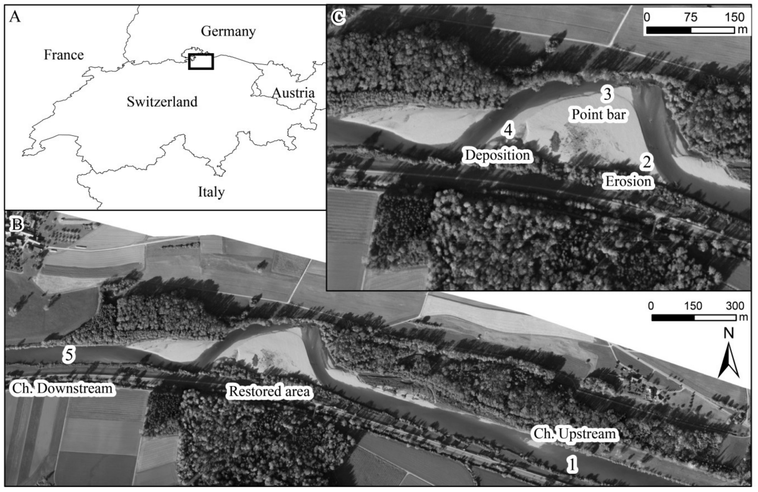
2.1. Study Site

We examined the Thur River, the largest river in Switzerland free of retention structures such us reservoir complexes. The Thur is a seventh order (Strahler order) perialpine river draining a catchment of 1730 km2 (Figure 1A), originating in the north-east alpine region of Switzerland from Mount Säntis (2502 m a.s.l.). Lacking large retention structures, the flow regime of the Thur is natural and dynamic, fluctuating from 3 to 900 m3/s with an average discharge of 47 m3/s (1995–2016 records). As with many rivers in Switzerland, the Thur was channelized with stone rip-rap in the 1890s for flood protection. In the 1990s, lateral rip-rap from different channel sections of 1–3 km in length was removed to allow the formation of new gravel bars and increase the hydrological connectivity between the river and riparian areas. In the 2002, a 1-km channel of protection (lateral levees, etc.) was removed along both banks of the river, allowing the river to widen using natural processes. This particular stretch was selected for the present study (Figure 1B). For more information on the restoration see [24,25].
The study reach was located in the lower part of the river (370 m a.s.l.), 12 km upstream of the confluence to the Rhine River. The 2-km long study area comprised the restored reach, which was subject to river widening, and channelized areas upstream and downstream of the restored section (Figure 1B). Channel width in the channelized reaches was about 50 m, while the maximum width in the restored area was 160 m. The slope of the reach was 0.16%. We selected five sampling sites in the study area (Figure 1B,C). Two sampling sites were located in the channelized reaches: one upstream (Site 1) and one downstream of the restored reach (Site 5). Three sampling sites were located along the main gravel bar in the restored reach: an erosional site (Site 2), a point bar site (Site 3), and a depositional site (Site 4).

2.2. Flow Regime Classification

Field surveys were conducted six times each in 2014 and 2015, monthly from early March to late November. Surveys were conducted when water levels were safe for access into the main channel (wadeable), but after flow pulses of different magnitude to account for hydrological variability (Figure 2). We used a daily discharge record from a gauging station located 7 km downstream of the sampling sites, at the municipality of Andelfingen, for flow and temperature data.
To study the effects of flow variation affecting each sample collection, each period was defined as the time elapsed between two sampling dates. As no defined period can be given for the first sampling date in both years, we used the average flow value from the previous 41 days (average duration of all periods). For categorization, nine hydrological descriptors were calculated for each period using the daily discharge data: mean, median, skewness, maximum, minimum, coefficient of variation, number of days flow was below the first quartile (low-flow events), number of days flow was above the third quartile (high-flow events), and number of days flow was above the sediment motion threshold (150 m3/s). The first and third quartiles (20 and 60 m3/s, respectively) were calculated from the 20-year record [4], while the sediment motion threshold value was taken from a previous study at the same site [26]. Each sampling period was categorized then into four flow classes according to similarity in the hydrological descriptors using Ward’s clustering: high, moderately high (Mod. High), intermediate, and low. We determined the number of classes from an inspection of the cluster dendrogram in a preliminary analysis to reasonably represent the flow regime in the study area (see Results).

2.3. Physico-Chemistry and Abiotic Hyporheic Measures

We measured local abiotic conditions including physical, chemical, and hyporheic attributes at each site on each sampling date. Physical attributes were represented by three variables: water depth (cm), velocity (cm/s), and median grain size of streambed sediments (stream d50; mm). An area of around 2 × 6 m near the left bank of the river was defined for each study reach. Due to erosion of the right bank, depths of over 2-m were impossible to sample using both banks. All measurements were randomly sampled within each plot, minimizing sampling disturbance between sites. Water depth was measured using a ruler (n = 5), water velocity at 0.6 depth (cm, n = 5) was measured using a portable velocity meter (MiniAir2, Schiltknecht AG, Gossau, Switzerland), and sediment size distribution was estimated by measuring the b-axis of 50 randomly-collected stones per site [27]. Further, a 0.5-litre water sample was collected at each site, returned to the laboratory, filtered (cellulose nitrate 0.45 μm, Sartorius Stedim Biotech) and analyzed for dissolved organic carbon (DOC; mg C/L), total nitrogen (TN; mg N/L), nitrate-N (NO3-N; mg N/L), and total phosphorus (TP; µg P/L) using methods in [28]. Electrical conductivity (µS/cm at 20 °C) was measured in the field using a portable meter (WTW model 340, Weilheim, Germany).
Hyporheic measures included particulate organic matter and median grain size of sediments used in sediment respiration experiments (see below), and vertical hydraulic gradient (VHG). Sediment used in respiration experiments was stored in plastic bags and kept frozen (−20 °C) until analysis. In the laboratory, coarse (CPOM) and fine organic matter (FPOM) was sieved (2 mm) from the sediments, dried at 60 °C, weighed, burned at 450 °C for 4 h, and reweighed to determine ash-free dry mass (AFDM). These sediments then were separated using a sieve column for quantifying grain size fractions >8 mm, 8–4 mm, 4–2 mm, 2–1 mm, 1–63 µm, and <63 µm. Median grain size (Hypo-d50, mm) was calculated using Gradistat v8 [29]. Vertical hydraulic gradient was measured in situ to characterize groundwater–streamwater exchange direction and magnitude. Minipiezometers were driven to a depth of ca. 50 cm into the streambed [30]. Positive values above stream-water surface levels indicated upwelling conditions, while negative values indicated downwelling conditions.

2.4. Sediment Respiration and Primary Production

Hyporheic sediment respiration (SR; mg O2 kg−1 sed h−1), a proxy for hyporheic organic matter processing, was measured in-situ following methods in [31]. Change in O2 concentration (mg/L) was measured overtime in sealed Plexiglas tubes (n = 3) half-filled with hyporheic sediments (5 to 20 cm depth, sieved <8 mm as standard protocol) and then filled with stream water. Surface sediments (first 5 cm of sediments) were excluded to avoid effects on respiration by autotrophs (after [32]). Sediment sampling locations were selected randomly within the study plot. A portable oxygen meter (Hach HQ40d connected to a LD0101 oxygen probe) was used to measure oxygen concentration and temperature in each tube before and after incubation. Hyporheic sediment respiration was calculated based on the consumption of O2 in the tube and the weight of sediment (R, mg O2 kg−1 sed h−1) and then normalized by a reference temperature (20 °C) to account for seasonal variation [33].
Periphyton biomass (AFDM, g/m2) and chlorophyll concentration (Chl-a, mg/m2) were measured as a proxy for primary production from five random cobbles collected from the streambed, stored in plastic bags, and kept frozen at −20 °C until processed. Periphyton was scrubbed from the surface of each stone using a metal brush, the slurry collected, volume measured, and divided into two sub-samples. Both sub-samples were filtered using Whatman GF/F filters. One filter was dried at 60 °C, weighed, combusted at 450 °C and reweighed for periphyton biomass estimation as AFDM. Surface area of each stone was calculated by wrapping the stone with aluminum foil and using a weight-to-area relationship [34]. The second filter was extracted for 7 min in 90% ethanol at 70 °C, and chlorophyll concentration measured by high performance liquid chromatography [35].

2.5. Macroinvertebrate Density and Taxa Richness

Benthic macroinvertebrates were randomly collected (n = 3, at each site and date) using a Hess sampler (250-um mesh, 0.04 m2 area) and preserved with 70% ethanol. Due to the characteristics of the river and the size of our study plots at a site, local habitats within each plot were relatively homogeneous. In the laboratory, collected individuals were hand-picked and identified to family level (Ephemeroptera, Plecoptera, Trichoptera, Diptera, Coleoptera, Gastropoda, Crustacea, Isopoda, and Odonata) or subclass level (Oligochaeta) and their abundances counted using a stereomicroscope (10× magnification). Macroinvertebrate density (individuals/m2) and taxa richness were calculated from the dataset.

2.6. Statistical Analysis

Two-way analysis of variance (ANOVA) was used to test if measured variables differed and interacted among sites (1–5) and flow classes (high, moderately high, intermediate, low) [36]. For better interpretation of the results, sites were re-grouped as restored (Sites 2–4) and non-restored sites (Sites 1 and 5), and the coefficient of variation (CV, defined as the standard deviation/mean) was used to examine the temporal variation of each variable within an area. Variation partitioning was used to determine the relative importance of sites and flow classes on the variation in ecosystem structure and function (various measures), except for macroinvertebrate community composition. The main ecosystem variables were explained individually by linear regression using the ‘varpart’ function [37] in the ‘vegan’ package of R software [38]. An ANOVA-like permutation test using the function ‘anova.rda’ then was used to evaluate the different partitions of each variable. A non-metric multidimensional scaling (NMDS) based on Bray–Curtis distance and calculated on log10(x + 1) transformed macroinvertebrate densities was used to examine changes in macroinvertebrate community composition followed by an analysis of similarity (ANOSIM), to test for among-group differences. All analyses were carried out using the R statistical computing software [38].

3. Results

3.1. Flow Classes

Ward’s cluster classification resulted in 4 flow classes. The high (n = 4) class showed the highest values of almost every flow indicator except for minimum discharge and low-flow events, followed by moderately high (n = 4), intermediate (n = 2), and low (n = 2) (Table 1). Periods were classified mainly by seasonality, but differences between 2014 (wet) and 2015 (dry) also contributed to classify intermediate and low classes (Figure 2). Maximum water temperature was 26.6 °C in July 2015 and minimum was 0.8 °C in December 2014.

3.2. Abiotic Factors

All collected data are summarized in Table 2. Statistical differences among sites were found in stream-d50, FPOM, CPOM, Hypo-d50, and VHG (Table 3). Their variability also was explained by flow class either directly or interactively with site, indicating that substrate size and hyporheic measures were influenced by de-channelization together with flow. Chemical variables (DOC, TN, and TP) were not explained by site but by flow class, indicating spatial homogeneity at the reach scale and intra-annual variation associated with flow.

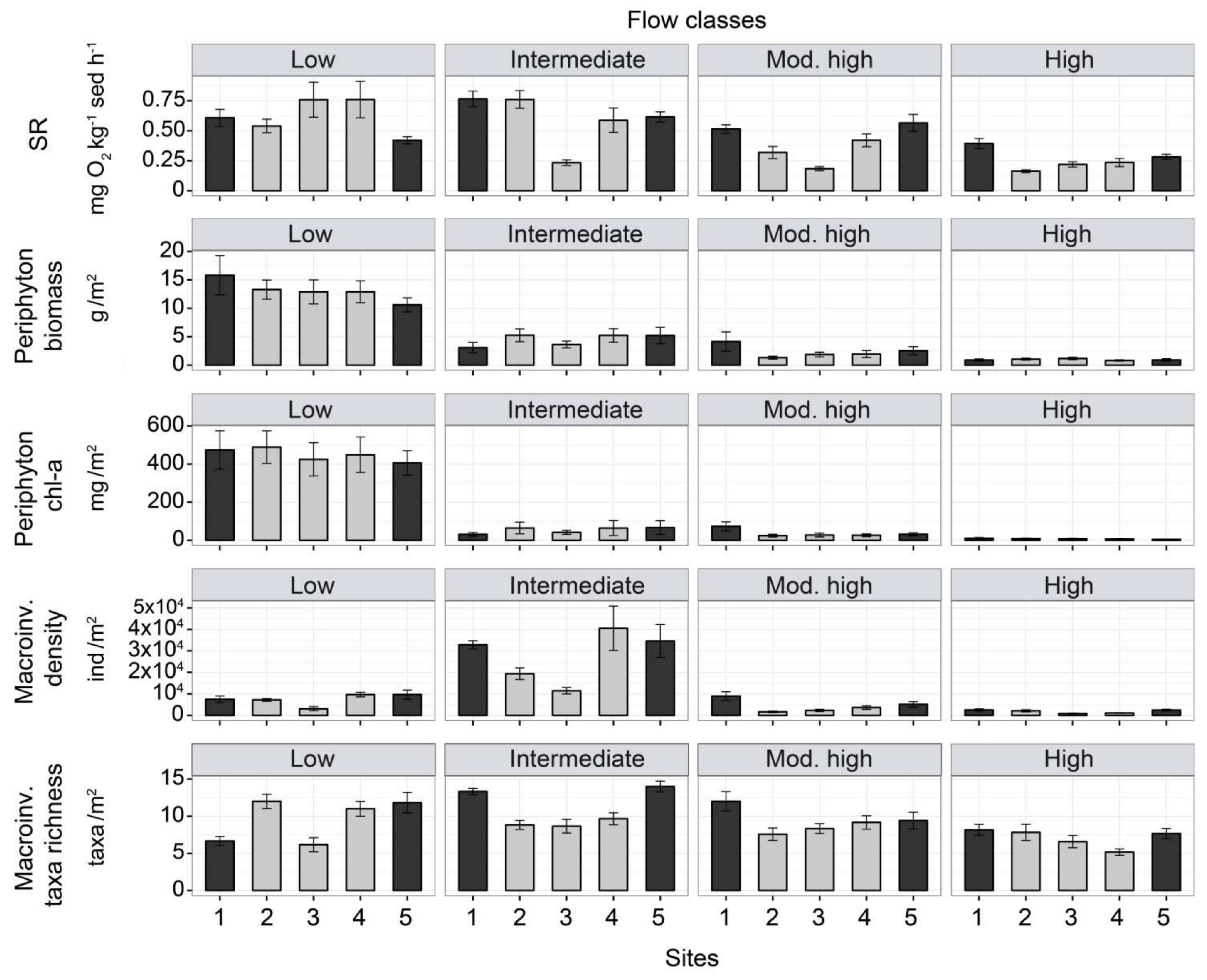
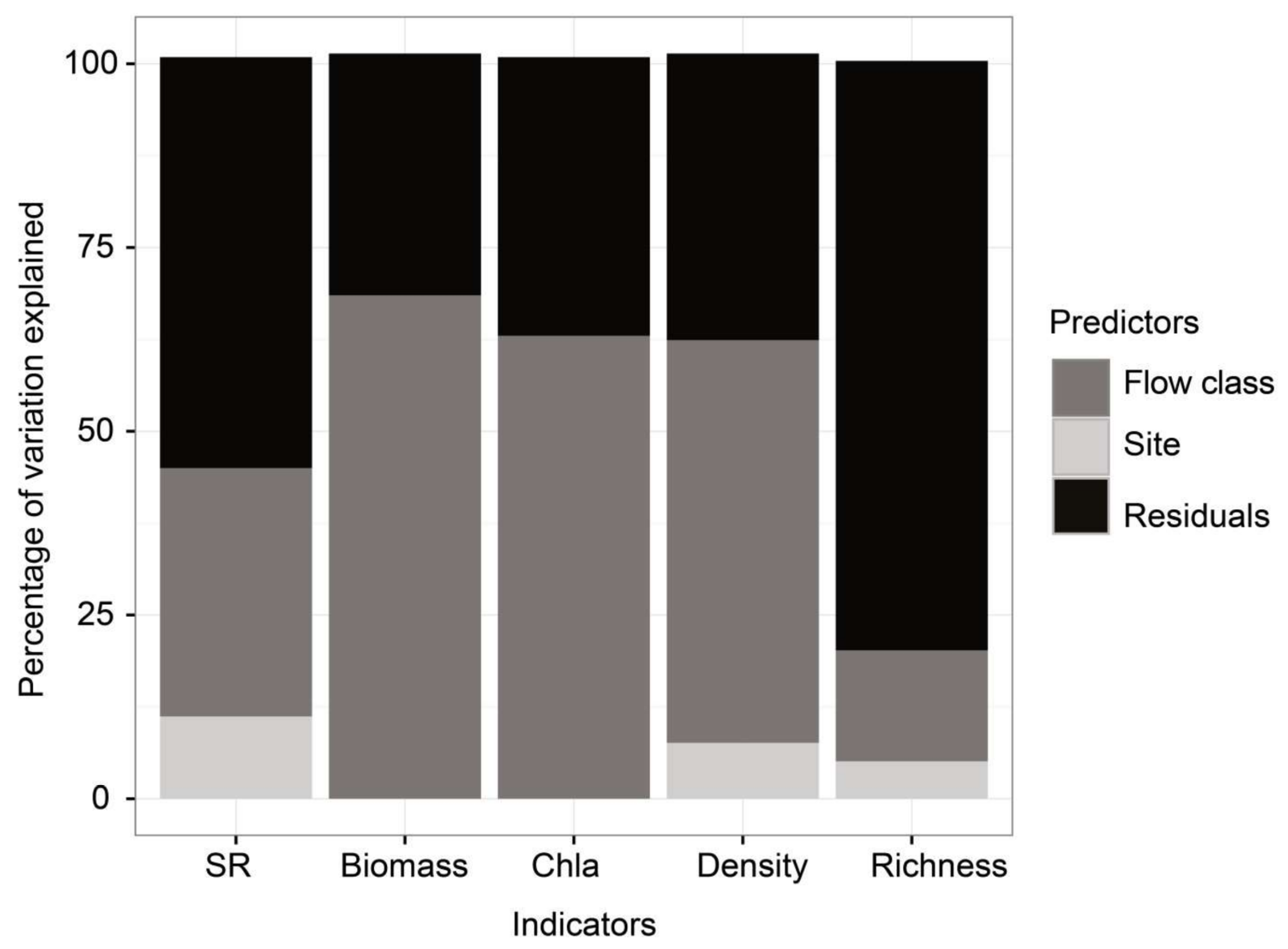
3.3. Ecosystem Function

Sediment respiration (SR) ranged from 0.10 to 1.39 (mg O2 kg−1 sed h−1) and differed among sites, flow classes and their interactions (all p < 0.01, Table 3), indicating that the spatial patterns of SR differed according to flow class. For instance, SR was lowest and spatially homogeneous for flow class high, while SR became higher and spatially heterogeneous in the other flow classes (Figure 3). SR at non-restored sites showed less variation among flow classes than restored sites (CV = 40% and 71%, respectively). Among restored sites, the temporal variability of SR was highest at the point bar (Site 3). Variation partitioning revealed a stronger influence of flow class (34%) than of site (11%) (Figure 4). Variation in periphyton AFDM and Chl-a was explained only by flow class (p < 0.01; >60% according to variance partitioning) (Figure 4, Table 3). Primary production was highest in flow class low (up to 22 g/m2 AFDM, >500 mg/m2 Chl-a) and extremely low (near 0) in the other flow classes.

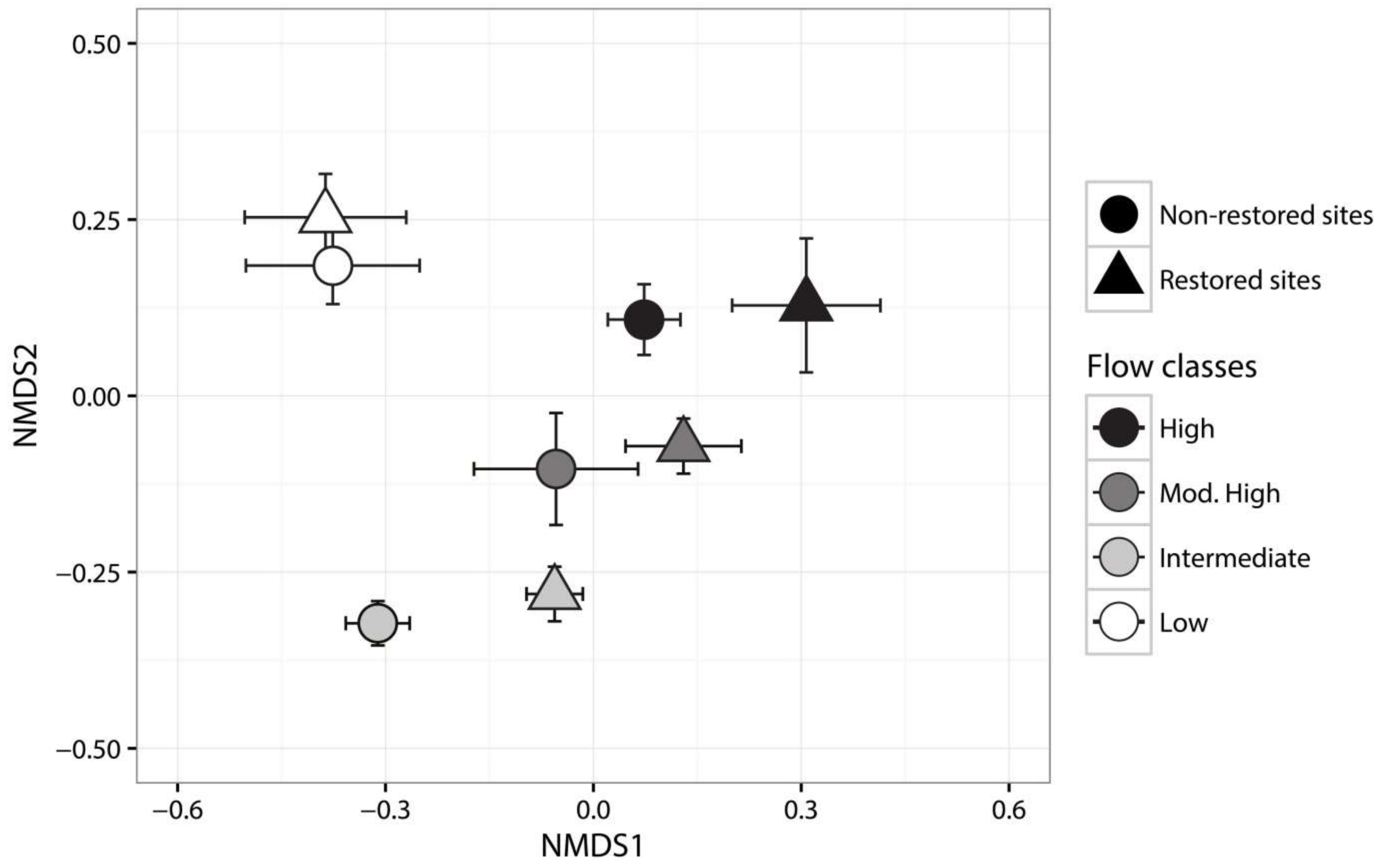
3.4. Ecosystem Structure

Macroinvertebrate density and taxa richness were significantly different among sites and flow classes (p < 0.01) (Figure 3). Taxa richness also was explained by their interaction (p = 0.02). Densities ranged from <100 to over 25,000 ind m−2. Erosional and point bar areas (Sites 2 and 3) had lower density and taxa richness than the other sites, while non-restored sites (Sites 1 and 5) had slightly higher densities and richness than restored sites (Figure 3). Density CV was higher in restored sites (176%) than in non-restored sites (124%), whereas richness CVs were the same for both (38%). The variation in macroinvertebrate density and richness was explained best by flow class (55 and 15%, respectively) and site (8% and 5%, respectively) (Figure 4).
NMDS analysis (stress = 0.21; Figure 5) showed a difference in macroinvertebrate composition among flow classes (ANOSIM by groups, R = 0.37, p = 0.001). Assemblages shifted in composition from class high to mod to intermediate along both NMDS axes, and a clearly different grouping was evident for class low (Figure 5). Restored and non-restored site assemblages were not statistically different in each flow class (ANOSIM, R = 0, p = 0.5), although the difference between restored and non-restored sites were distinctive owing to their position along axis-1 (Figure 5). The differences between restored and non-restored site communities were constant despite flow type.

4. Discussion

We investigated the effect of channel protection removal (river widening) on ecosystem structure and function after 12 years in the Thur River, Switzerland. Our results showed that (i) spatial and temporal variation in sediment respiration and macroinvertebrate taxonomic richness were driven by interactions between flow and restoration; (ii) riverbed measures including substrate size, organic matter content, and groundwater–surface water interchange were changed due to restoration, but (iii) water chemistry, hydraulic conditions, and primary production were not affected by restoration.
These findings are important because river restoration often focuses on abiotic conditions with little attention on biotic assemblages or ecosystem function [39,40,41]. Our study revealed that abiotic measures, except channel morphology, changed only marginally but ecosystem structure and function showed complex responses in relation to flow-restoration interactions that are usually absent in channelized rivers due to more stable conditions in sediment and flow regimes. These results highlight designing restoration projects using a more holistic perspective including biotic and functional measures [42] at multiple temporal (intra- and inter-annual) and spatial (habitat, reach) scales, which will help assess results of a project beyond the before/after design.
We found a more abundant and richer macroinvertebrate assemblage, on average, in non-restored than restored sites. These results are in line with previous studies showing marginal changes in macroinvertebrate assemblages in restored reaches despite enhanced habitat heterogeneity [43,44]. The greater disturbance in restored sites, in terms or sediment movement and deposition, may be one explanation for the differences in our study. Other potential explanations for this response by macroinvertebrates include irrelevant spatial scales of management actions, time limitations for assemblages to show a response, or ignoring other stressors in the same river [45]. Further, spatial differences in community composition should be considered. For instance, the community was dominated by snails (Hydrobiidae, Valvatidae, and Planorbidae), Odonata (Gomphidae, Corduliidae), and isopods (Ashellidae) in flow class low, while these groups were absent in the other flow classes (results not shown). Nevertheless, the reduction in abundance and richness does not necessarily lead us to conclude that the restoration had an overall negative impact because the aim of the project was successfully achieved by re-generating flow–sediment interactions.
Measures of ecosystem function revealed various responses to restoration. Here, restoration resulted in the enhancement of spatio-temporal dynamics in sediment respiration due to the interaction between flow and sediment dynamics. Sediment movement in the restored sites was affected differently by the different classes of flow events, whereas this effect on sediment movement was not evident in the non-restored sites, likely because the non-restored sites were more stable and lack the interaction between flow and sediment movement of the streambed. Importantly, this interaction may indicate re-establishment of organic matter processing at the reach scale [46]. Periphyton biomass (AFDM and Chl-a) showed no difference due to restoration but differed among flow classes, likely reflecting greater susceptibility to physical disturbance by scouring and sheer stress [26,47]. The fact that this response occurred in restored and non-restored sites suggests a remarkably low resistance of surface biofilms to spates [26], despite spatial differences in river morphology and bed heterogeneity.
Hyporheic sediment respiration (SR) also showed different responses to flow classes among sites. SR was less variable over time in non-restored relative to restored sites. The lack of natural disturbance in rivers may have general consequences that could lead to a regime shift in habitats [48], such as an increase in (in)organic matter and less organic carbon transported downstream [49]. Restoration clearly increased the heterogeneity in ecosystem function of hyporheic sediments in the Thur River.
Exchange between the water column and channel bed and river banks (vertical and lateral linkages) can affect water quality because these are biogeochemically active areas where organic matter decomposition and nitrogen removal occurs [50,51]. Our results showed that water chemistry was not influenced by the restoration, and is in agreement with previous studies [52,53]. Water chemistry was best explained by intra-annual flow variability, indicating that river water chemistry responds mainly to large-scale processes such as snowmelt water intrusion or major precipitation events [54] as well as large-scale patterns in river morphology such as meandering [55]. Here, the length of the restored stretch (ca. 500 m) may have been too short to detect or cause changes in water chemistry. Overall, the results demonstrate a positive response of rivers to channel widening actions by facilitating sediment flow relations in restored sections.

Acknowledgments

We thank C. Jolidon and S. Blaser for field and lab assistance. We thank the AUA lab, EAWAG, for chemical analysis of water samples. Pictures were provided by Amt für Umwelt, Kanton Thurgau/BSF Swissphoto. This study was funded by the BAFU Project “Wasserbau & Ökologie”.

Author Contributions

E.J.M., M.D. and C.T.R. conceived and designed the research; E.J.M. and C.T.R. performed the sampling, E.J.M. analyzed the data; M.R. contributed analysis tools; E.J.M., M.R., M.D. and C.T.R. wrote the manuscript.

Conflicts of Interest

The authors declare no conflict of interest.

References

  1. Resh, V.H.; Brown, A.V.; Covich, A.P.; Gurtz, M.E.; Li, H.W.; Minshall, G.W.; Reice, S.R.; Sheldon, A.L.; Wallace, J.B.; Wissmar, R.C. The role of disturbance in stream ecology. J. N. Am. Benthol. Soc. 1988, 7, 433–455. [Google Scholar] [CrossRef]
  2. Poff, N.L.; Ward, J.V. Implications of streamflow variability and predictability for lotic community structure: A regional analysis of streamflow patterns. Can. J. Fish. Aquat. Sci. 1989, 46, 1805–1818. [Google Scholar] [CrossRef]
  3. Bunn, S.E.; Arthington, A.H. Basic principles and ecological consequences of altered flow regimes for aquatic biodiversity. Environ. Manag. 2002, 30, 492–507. [Google Scholar] [CrossRef]
  4. Richter, B.D.; Baumgartner, J.V.; Powell, J.; Braun, D.P. A method for assessing hydrologic alteration within ecosystems. Conserv. Boil. 1996, 10, 1163–1174. [Google Scholar] [CrossRef]
  5. Lytle, D.A.; Poff, N.L. Adaptation to natural flow regimes. Trends Ecol. Evol. 2004, 19, 94–100. [Google Scholar] [CrossRef] [PubMed]
  6. Wood, P.J.; Armitage, P.D. The response of the macroinvertebrate community to low-flow variability and supra-seasonal drought within a groundwater dominated stream. Arch. Hydrobiol. 2004, 161, 1–20. [Google Scholar] [CrossRef]
  7. Iwasaki, Y.; Ryo, M.; Sui, P.; Yoshimura, C. Evaluating the relationship between basin-scale fish species richness and ecologically relevant flow characteristics in rivers worldwide. Freshw. Biol. 2012, 57, 2173–2180. [Google Scholar] [CrossRef]
  8. Wohl, E.E.; Bledsoe, B.P.; Jacobson, R.B.; Poff, N.L.; Rathburn, S.L.; Walters, D.M.; Wilcox, A.C. The natural sediment regime in rivers: Broadening the foundation for ecosystem management. Bioscience 2015, 65, 358–371. [Google Scholar] [CrossRef]
  9. Southwood, T.R.E. Habitat, the template for ecological strategies? J. Anim. Ecol. 1977, 46, 337–365. [Google Scholar] [CrossRef]
  10. Lytle, D.A.; Bogan, M.T.; Finn, D.S. Evolution of aquatic insect behaviours across a gradient of disturbance predictability. Proc. R. Soc. Lond. B Biol. Sci. 2008, 275, 453–462. [Google Scholar] [CrossRef] [PubMed]
  11. Jones, J.I.; Murphy, J.F.; Collins, A.L.; Sear, D.A.; Naden, P.S.; Armitage, P.D. The impact of fine sediment on macroinvertebrates. River Res. Appl. 2012, 28, 1055–1071. [Google Scholar] [CrossRef]
  12. Merritt, D.M. Reciprocal relations between riparian vegetation, fluvial landforms, and channel processes. In Treatise on Geomorphology; Academic Press: Cambridge, MA, USA, 2013; pp. 219–243. [Google Scholar]
  13. Benke, A.C. Importance of flood regime to invertebrate habitat in an unregulated river-floodplain ecosystem. N. Am. Benthol. Soc. 2001, 20, 225–240. [Google Scholar] [CrossRef]
  14. Surian, N.; Rinaldi, M. Morphological response to river engineering and management in alluvial channels in Italy. Geomorphology 2003, 50, 307–326. [Google Scholar] [CrossRef]
  15. Brandt, S.A. Classification of geomorphological effects downstream of dams. Catena 2000, 40, 375–401. [Google Scholar] [CrossRef]
  16. Tena, A.; Batalla, R.J. The sediment budget of a large river regulated by dams (The lower River Ebro, NE Spain). J. Soils Sediments 2013, 13, 966–980. [Google Scholar] [CrossRef]
  17. Zeh, W.H.; Könitzer, C.; Bertiller, A. Structures of Watercourses in Switzerland; Swiss Federal Office of Environment: Bern, Switzerland, 2009. [Google Scholar]
  18. Lach, J.; Wyzga, B. Channel incision and flow increase of the upper Wisłoka River, southern Poland, subsequent to the reafforestation of its catchment. Earth Surf. Process. Landf. 2002, 27, 445–462. [Google Scholar] [CrossRef]
  19. Tockner, K.; Stanford, J.A. Riverine floodplains: Present state and future trends. Environ. Conserv. 2002, 29, 308–330. [Google Scholar] [CrossRef]
  20. Gregory, K.J. The human role in changing river channels. Geomorphology 2006, 79, 172–191. [Google Scholar] [CrossRef]
  21. European-Commission. Directive 2000/60/EC of the European Parliament and of the Council of 23 October 2000 establishing a framework for community action in the field of water policy. Off. J. Eur. Community 2000, L327, 1–72.
  22. Yarnell, S.M. Quantifying physical habitat heterogeneity in an ecologically meaningful manner: A case study of the habitat preferences of the foothill yellow-legged frog (Rana boylii). In Landscape Ecology Research Trends; Dupont, A., Jacobs, H., Eds.; Nova Science: Hauppauge, NY, USA, 2008; pp. 89–112. [Google Scholar]
  23. Richards, K.; Brasington, J.; Hughes, F. Geomorphic dynamics of floodplains: Ecological implications and a potential modelling strategy. Freshw. Biol. 2002, 47, 559–579. [Google Scholar] [CrossRef]
  24. Seidl, R.; Stauffacher, M. Evaluation of river restoration by local residents. Water Resour. Res. 2013, 10, 7077–7087. [Google Scholar] [CrossRef]
  25. Schirmer, M.; Luster, J.; Linde, N.; Perona, P.; Mitchell, E.; Andrew Barry, D.; Hollender, J.; Cirpka, O.; Schneider, P.; Vogt, T.; et al. Morphological, hydrological, biogeochemical and ecological changes and challenges in river restoration—The Thur River case study. Hydrol. Earth Syst. Sci. 2014, 18, 2449–2462. [Google Scholar] [CrossRef] [Green Version]
  26. Uehlinger, U. Resistance and resilience of ecosystem metabolism in a flood-prone river system. Freshw. Biol. 2000, 45, 319–332. [Google Scholar] [CrossRef]
  27. Wolman, M.G. A method of sampling coarse river-bed material. EOS Trans. Am. Geophys. Union 1954, 35, 951–956. [Google Scholar] [CrossRef]
  28. Tockner, K.; Malard, F.; Burgherr, P.; Robinson, C.T.; Uehlinger, U.; Zah, R.; Ward, J.V. Characteristics of channel types in a glacial floodplain ecosystem (Val Roseg, Switzerland). Arch. Hydrobiol. 1997, 140, 430–463. [Google Scholar]
  29. Blott, S.J.; Pye, K. GRADISTAT: A grain size distribution and statistics package for the analysis of unconsolidated sediments. Earth Surf. Process. Landf. 2001, 26, 1237–1248. [Google Scholar] [CrossRef]
  30. Baxter, C.V.; Hauer, F.R.; Woessner, W.W. Measuring groundwater-stream water exchange: New techniques for installing minipiezometers and estimating hydraulic conductivity. Trans. Am. Fish. Soc. 2003, 132, 493–502. [Google Scholar] [CrossRef]
  31. Uehlinger, U.; Naegeli, M.W.; Fisher, S.G. A heterotrophic desert stream? The role of sediment stability. West. N. Am. Nat. 2002, 62, 466–473. [Google Scholar]
  32. Doering, M.; Uehlinger, U.; Ackermann, T.; Woodtle, M.; Tockner, K. Spatiotemporal heterogeneity of soil and sediment respiration in a river-floodplain mosaic (Tagliamento, NE Italy). Freshw. Biol. 2011, 56, 1297–1311. [Google Scholar] [CrossRef]
  33. Naegeli, W.; Uehlinger, U. Contribution of the hyporheic zone to ecosystem metabolism in a prealpine gravel-bed river. J. N. Am. Benthol. Soc. 1997, 16, 794–804. [Google Scholar] [CrossRef]
  34. Bergey, E.A.; Getty, G.M. A review of methods for measuring the surface area of stream substrates. Hydrobiologia 2006, 556, 7–16. [Google Scholar] [CrossRef]
  35. Meyns, S.; Illi, R.; Ribi, B. Comparison of chlorophyll—A analysis by HPLC and spectrophotometry: Where do the differences come from? Arch. Hydrobiol. 1994, 132, 129–139. [Google Scholar]
  36. Vischer, D.; Hager, W.H.; Casanova, C.; Joos, B.; Lier, P.; Martini, O. Bypass tunnels to prevent reservoir sedimentation Q74 R37. In Proceedings of the 19th ICOLD Congress, Florence, Italy, 26–30 May 1997. [Google Scholar]
  37. Peres-Neto, P.R.; Legendre, P.; Dray, S.; Borcard, D. Variation partitioning of species data matrices: Estimation and comparison of fractions. Ecology 2006, 87, 2614–2625. [Google Scholar] [CrossRef]
  38. R Development Core Team. R: A Language and Environment for Statistical Computing; R Foundation for Statistical Computing: Vienna, Austria, 2015. [Google Scholar]
  39. Muotka, T.; Paavola, R.; Haapala, A.; Novikmec, M.; Laasonen, P. Long-term recovery of stream habitat structure and benthic invertebrate communities from in-stream restoration. Biol. Conserv. 2002, 105, 243–253. [Google Scholar] [CrossRef]
  40. Lepori, F.; Palm, D.; Brännäs, E.; Malmqvist, B. Does restoration of structural heterogeneity in streams enhance fish and macroinvertebrate diversity? Ecol. Appl. 2005, 15, 2060–2071. [Google Scholar] [CrossRef]
  41. Jähnig, S.C.; Brabec, K.; Buffagni, A.; Erba, S.; Lorenz, A.W.; Ofenböck, T.; Verdonschot, P.F.M.; Hering, D. A comparative analysis of restoration measures and their effects on hydromorphology and benthic invertebrates in 26 central and southern European rivers. J. Appl. Ecol. 2010, 47, 671–680. [Google Scholar] [CrossRef]
  42. Palmer, M.A.; Menninger, H.L.; Bernhardt, E.S. River restoration, habitat heterogeneity and biodiversity: A failure of theory or practice? Freshw. Biol. 2010, 55, 205–222. [Google Scholar] [CrossRef]
  43. Bernhardt, E.S.; Palmer, M.A. River restoration: The fuzzy logic of repairing reaches to reverse catchment scale degradation. Ecol. Appl. 2011, 21, 1926–1931. [Google Scholar] [CrossRef] [PubMed]
  44. Violin, C.R.; Cada, P.; Sudduth, E.B.; Hassett, B.A.; Penrose, D.L.; Bernhardt, E.S. Effects of urbanization and urban stream restoration on the physical and biological structure of stream ecosystems. Ecol. Appl. 2011, 21, 1932–1949. [Google Scholar] [CrossRef] [PubMed]
  45. Haase, P.; Hering, D.; Jähnig, S.C.; Lorenz, A.W.; Sundermann, A. The impact of hydromorphological restoration on river ecological status: A comparison of fish, benthic invertebrates, and macrophytes. Hydrobiologia 2012, 704, 475–488. [Google Scholar] [CrossRef]
  46. Robinson, C.T.; Uehlinger, U. Experimental floods cause ecosystem regime shift in a regulated river. Ecol. Appl. 2008, 18, 511–526. [Google Scholar] [CrossRef] [PubMed]
  47. Uehlinger, U.; Kawecka, B.; Robinson, C.T. Effects of experimental floods on periphyton and stream metabolism below a high dam in the Swiss Alps (River Spöl). Aquat. Sci. 2003, 65, 199–209. [Google Scholar] [CrossRef]
  48. Scheffer, M.; Carpenter, S.; Foley, J.A.; Folke, C.; Walker, B. Catastrophic shifts in ecosystems. Nature 2001, 413, 591–596. [Google Scholar] [CrossRef] [PubMed]
  49. Aristi, I.; Arroita, M.; Larrañaga, A.; Ponsatí, L.; Sabater, S.; von Schiller, D.; Elosegi, A.; Acuña, V. Flow regulation by dams affects ecosystem metabolism in Mediterranean rivers. Freshw. Biol. 2014, 59, 1816–1829. [Google Scholar] [CrossRef]
  50. Findlay, S. Importance of surface-subsurface exchange in stream ecosystems: The hyporheic zone. Limnol. Oceanogr. 1995, 40, 159–164. [Google Scholar] [CrossRef]
  51. Battin, T.J.; Kaplan, L.A.; Newbold, J.D.; Hendricks, S.P. A mixing model analysis of stream solute dynamics and the contribution of a hyporheic zone to ecosystem function. Freshw. Biol. 2003, 48, 995–1014. [Google Scholar] [CrossRef]
  52. Boulton, A.J.; Findlay, S.; Marmonier, P.; Stanley, E.H.; Valett, H.M. The functional significance of the hyporheic zone in streams and rivers. Annu. Rev. Ecol. Syst. 1998, 29, 59–81. [Google Scholar] [CrossRef]
  53. Fernald, A.G.; Landers, D.H.; Wigington, P.J. Water quality changes in hyporheic flow paths between a large gravel bed river and off-channel alcoves in Oregon, USA. River Res. Appl. 2006, 22, 1111–1124. [Google Scholar] [CrossRef]
  54. Poff, L.N.; Allan, J.D.; Bain, M.B.; Karr, J.R.; Prestegaard, K.L.; Richter, B.D.; Sparks, R.E.; Stormberg, J.C. The natural flow regime. Bioscience 1997, 47, 769–784. [Google Scholar] [CrossRef]
  55. Gomez-Velez, J.D.; Harvey, J.W. A hydrogeomorphic river network model predicts where and why hyporheic exchange is important in large basins. Geophys. Res. Lett. 2014, 41, 6403–6412. [Google Scholar] [CrossRef]
Figure 1. (A) Location of study area in Switzerland. (B) General view of the study reach, including channelized areas upstream (Site 1) and downstream (Site 5) of the restored area. (C) Detail picture of the main restored gravel bar and study sites 2–4. Ch = channelized.
Water 10 00439 g001
Figure 2. Hydrograph of the Thur River in 2014–2015. Black lines represent flow classes of the period affecting each sampling campaign (Mod. High = Moderately High).
Water 10 00439 g002
Figure 3. Ecosystem structure and function measures by site and flow class (average ± standard error). Black bars (Sites 1 and 5) represent non-restored sites, while grey bars (Sites 2–4) represent restored sites. SR = sediment respiration; Macroinv = macroinvertebrate; Mod. High = moderately high.
Water 10 00439 g003
Figure 4. Partitioning variation of ecosystem structure and function measures (percentage of variation explained by flow class and site). All proportions of explained variance were significant (p < 0.05). SR = sediment respiration; Chl-a = periphyton chlorophyll; Density = macroinvertebrate density; and Richness = macroinvertebrate taxonomic richness.
Water 10 00439 g004
Figure 5. Community composition in NMDS ordination space based on macroinvertebrate densities. Symbols represent samples for different flow classes in restored or non-restored sites.
Water 10 00439 g005
Table 1. Summarized characteristics of hydrological indicators of each flow class (average ± standard error). Note that mean, median, and maximum discharge were not used for classification to avoid multicollinearity.
Flow Classes
IndicatorHighMod. HighIntermediateLow
n4422
Mean (m3/s)76.4 ± 7.241.2 ± 3.932.7 ± 0.614.1 ± 0.2
Median (m3/s)49.7 ± 7.832.4 ± 3.031.0 ± 0.412.8 ± 0.5
Skewness1.6 ± 0.11.3 ± 0.01.1 ± 0.01.1 ± 0.0
Max (m3/s)281.0 ± 15.5175.8 ± 24.249.9 ± 1.735.5 ± 6.2
Min (m3/s)23.5 ± 3.815.1 ± 2.023.7 ± 2.26.8 ± 0.5
Days < first q1.8 ± 0.97.5 ± 3.00.0 ± 0.041.5 ± 8.1
Days > third q15.5 ± 2.88.0 ± 2.30.0 ± 0.00.0 ± 0.0
CV0.9 ± 0.00.8 ± 0.10.2 ± 0.00.4 ± 0.1
Days disrupt3.8 ± 1.01.0 ± 0.50.0 ± 0.00.0 ± 0.0
Note: Days < first q = numbers of days discharge below first quartile; Days > third q = numbers of days discharge above third quartile; CV = coefficient of variation; Days disrupt = numbers of days discharge above sediment motion threshold.
Table 2. Physico-chemical and hyporheic zone characterization of the study sites and flow classes (average ± standard error).
VelDepthStream d50DOCTNNO3-NTPCondFPOMCPOMHypo-d50VHG
Sitem/scmcmmg C/Lmg N/Lmg N/Lµg P/LµS/cm 20 °Cg/kg sedg/kg sedcmcm/cm
10.35 ± 0.137.8 ± 3.73.4 ± 0.32.3 ± 0.12.4 ± 0.12.2 ± 0.137.5 ± 3.5422.3 ± 13.34.0 ± 0.10.18 ± 0.024.8 ± 0.10.12 ± 0.06
20.55 ± 0.125.0 ± 2.24.2 ± 0.52.3 ± 0.12.4 ± 0.12.2 ± 0.137.9 ± 3.8423.8 ± 13.34.5 ± 0.20.10 ± 0.023.8 ± 0.2−0.06 ± 0.03
30.21 ± 0.127.5 ± 3.13.1 ± 0.32.3 ± 0.12.4 ± 0.12.2 ± 0.138.3 ± 3.8425.4 ± 13.14.0 ± 0.10.24 ± 0.053.2 ± 0.20.08 ± 0.03
40.27 ± 0.127.2 ± 2.71.9 ± 0.32.3 ± 0.12.4 ± 0.12.2 ± 0.137.5 ± 3.8423.4 ± 13.44.2 ± 0.10.16 ± 0.033.0 ± 0.20.04 ± 0.03
50.23 ± 0.118.3 ± 1.33.5 ± 0.32.2 ± 0.12.4 ± 0.12.2 ± 0.139.6 ± 3.8423.9 ± 13.04.1 ± 0.10.15 ± 0.024.4 ± 0.20.22 ± 0.03
Flow class
High0.39 ± 0.127.1 ± 2.32.7 ± 0.21.9 ± 0.12.2 ± 0.12.1 ± 0.138.4 ± 1.8421.8 ± 8.33.9 ± 0.10.14 ± 0.023.9 ± 0.20.11 ± 0.02
Mod. highn.a.31.2 ± 2.62.9 ± 0.22.4 ± 0.12.3 ± 0.12.2 ± 0.145.1 ± 2.3421.1 ± 8.74.4 ± 0.10.15 ± 0.023.8 ± 0.20.04 ± 0.03
Intermediaten.a.n.a.n.a.2.6 ± 0.12.8 ± 0.22.5 ± 0.143.9 ± 2.8421.0 ± 22.33.9 ± 0.10.10 ± 0.024.0 ± 0.2n.a.
Low0.22 ± 0.121.3 ± 1.74.2 ± 0.32.3 ± 0.12.5 ± 0.12.3 ± 0.118.2 ± 0.7435.8 ± 12.44.6 ± 0.10.31 ± 0.053.6 ± 0.30.08 ± 0.04
Note: Vel = velocity; Stream-d50 = streambed median sediment size; DOC = dissolved organic carbon ; TN = total nitrogen; NO3-N = Nitrate-N; TP = total phosphorus; Cond = electrical conductivity; FPOM = Fine particulate organic matter; CPOM = Coarse particulate organic matter; Hypo-d50 = hyporheic median sediment size; VHG = vertical hydraulic gradient; n.a. = not available.
Table 3. Two way ANOVA results of the effects of site and flow class on all measured variables. Bold numbers indicate statistical significance (α = 0.05).
SiteFlow ClassSite * Flow Class
Abiotic factors
PhysicalVelocity0.070.040.36
Depth0.710.710.5
Stream-d50<0.01<0.010.43
ChemicalDOC0.99<0.010.99
TN0.99<0.011
NO3-N0.990.081
TP0.98<0.010.99
Cond0.990.861
HyporheicFPOM0.01<0.010.91
CPOM0.01<0.01<0.01
Hypo-d50<0.010.55<0.01
VHG<0.010.060.03
Ecosystem function
SR<0.01<0.01<0.01
Periphyton biomass0.93<0.010.49
Chl-a0.39<0.010.82
Ecosystem structure
Density<0.01<0.010.32
Richness<0.01<0.010.02
Note: Stream-d50 = streambed median sediment size; DOC = dissolved organic carbon; TN = total nitrogen; NO3-N = nitrate-N; TP = total phosphorus; Cond = electrical conductivity; FPOM = fine particle organic matter; CPOM = coarse particle organic matter; Hypo-d50 = hyporheic median sediment size; VHG = vertical hydraulic gradient; SR = sediment respiration; Chl-a = periphyton chlorophyll; Density = macroinvertebrate density; and Richness = macroinvertebrate taxonomic richness. * represents the interaction between site and flow class.

