Comparison of Pressure-Driven Formulations for WDN Simulation


Dipartimento di Ingegneria Civile e Architettura, Univ. of Pavia, Via Ferrata 3, 27100 Pavia, Italy
*
Author to whom correspondence should be addressed.
Water 2018, 10(4), 523; https://doi.org/10.3390/w10040523
Submission received: 24 March 2018
/
Revised: 17 April 2018
/
Accepted: 19 April 2018
/
Published: 21 April 2018
(This article belongs to the Special Issue Advances in Water Distribution Networks)
Abstract
:This paper presents the comparison of five pressure-driven formulations in the context of water distribution network (WDN) modelling. These formulations, which relate nodal outflow q to users to demands d and nodal pressure heads h, were implemented inside the global gradient algorithm for the snapshot solution of the equations concerning mass and energy conservation at WDN nodes and pipes, respectively. The modelling of leakage nodal outflows as a function of pressure was also considered. The applications concerned two case studies, in which nodal demands were suitably amplified to lower service pressure below the desired values. This was done to stress the effects of the pressure-driven dependence q(h) in the WDN. The results showed that the formulations tend to behave similarly in terms of nodal outflows. Compared to a widely used formulation, which features a q(h) relationship with derivative discontinuities, the other four formulations analyzed tend to guarantee faster algorithm convergence, above all for simple and poorly interconnected WDNs, due to their smooth q(h) relationship. The results in terms of nodal pressure heads can be very different, above all for low values of h.
1. Introduction
The traditional approach for simulating water distribution networks (WDNs) is the demand-driven approach (DDA) [1,2,3,4], in which nodal outflows are set equal to demands independently from service pressure. In this context, the solution of mass and energy balance equations enables determining nodal heads and pipe flows in either snapshot or extended-period simulations [5]. The DDA yields satisfying results in some applications, such as WDN design, in which service pressure is assumed to be larger than the desired value for full demand satisfaction. However, some abnormal operational scenarios [6], such as those occurring during pipe bursts, segment isolation, or excessive water use, may cause service pressure to fall below the desired value. In these scenarios, DDA was noticed to yield poor prediction of nodal heads and pipe flows in the WDN. To solve this issue, the pressure-driven approach (PDA) was proposed in [7] and then considered by numerous authors, e.g., [8,9,10,11,12,13,14,15,16,17,18,19,20,21,22]. In PDA, the ratio of nodal outflow to nodal demand can be expressed as a function of a nodal pressure head by using one of the numerous formulations available in the scientific literature [7,9,12,13,17,20].
Whereas lots of research was dedicated to setting up increasingly robust and efficient algorithms for WDN solution (e.g., [15,16,21]), the effects of the various formulations proposed in terms of WDN solution results and algorithm convergence speed have been analyzed marginally. This paper aims to contribute to this issue.
In the following sections, first the methodology is described, including the pressure-driven formulations considered and the model used for WDN solution. The methodology is followed by the applications to two case studies and by the conclusions of the work.
2. Materials and Methods
In the present section, the pressure-driven formulations compared are presented (Section 2.1) followed by the algorithm used for WDN resolution (Section 2.2).
2.1. Pressure-Driven Formulations
The pressure-driven formulations considered in this work to express the actual nodal outflow q as a function of the actual nodal pressure head h and demand d are those of Wagner et al. [9], Fujiwara and Li [12], Tucciarelli et al. [13], Tanyimboh and Templeman with default parameters [17], and with calibration proposed by Ciaponi et al. [20]. All formulations consider the definition of a desired pressure head hdes for full demand satisfaction. The Wagner et al. [9], Fujiwara and Li [12], and Tanyimboh and Templeman with default parameters [17] formulations also consider a minimum pressure head hmim to have outflow while the Tucciarelli et al. [13] and Ciaponi et al. [20] formulations were developed considering hmim = 0.
In the formulations of Wagner et al. [9], Fujiwara and Li [12], and Tucciarelli et al. [13], q/d = 0 and q/d = 1 for h ≤ hmin and h ≥ hdes, respectively.
For hmin ≤ h ≤ hdes, the Wagner et al. [9] formulation yields:
with coefficient γ usually set at 2 to re-obtain the same kind of relationship of the outflow through an orifice. Though being the most widely used, this formulation has the drawback of presenting derivative discontinuities for h = hmin and h = hdes. This drawback is overcome in the formulations of Fujiwara and Li [12] and Tucciarelli et al. [13].
Unlike the formulations of Wagner et al. [9], Fujiwara and Li [12], and Tucciarelli et al. [13], that of Tanyimboh and Templeman [17] is based on the following single smooth relationship, which holds for all of the values of h:
where, in absence of field data, the default values of the parameters Y and B are calculated through the following expressions:
Using the same structure as (4), Ciaponi et al. [20] developed statistically expressions for Y and B with the objective to reproduce, on average, the complex and varied set of phenomena governing the actual water delivery at each network node. The resulting formulation, proposed for flat sites, is:
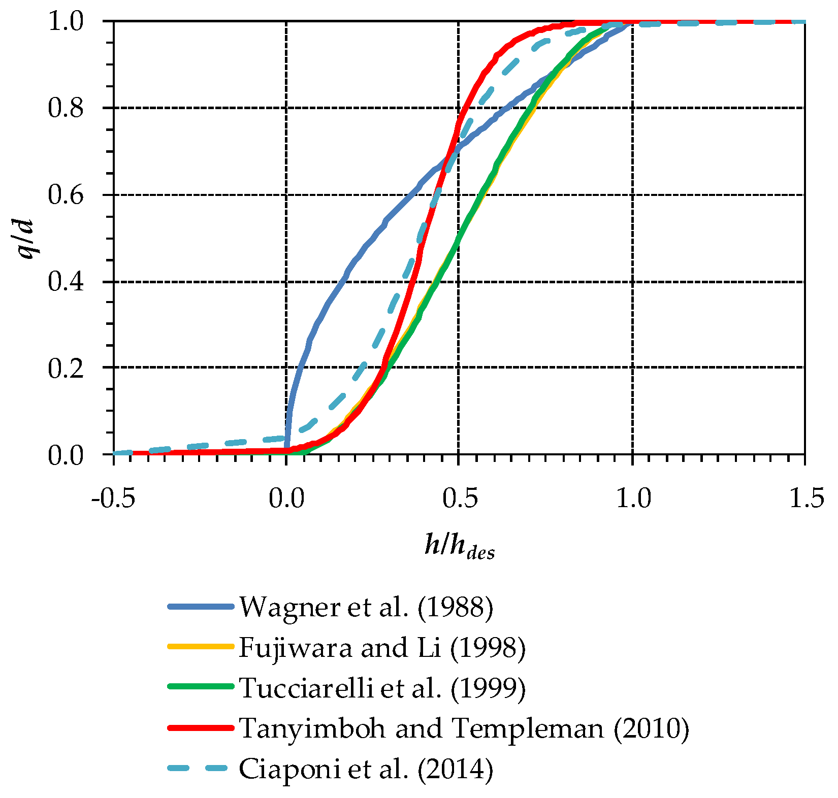
The graphical comparison of the five formulations presented above is reported in Figure 1 for hmin = 0 and hdes = 20, showing that the Fujiwara et al. [12] and Tucciarelli et al. [13] formulations give very similar values of q/d, which are lower than the other formulations over almost the entire range of h/hdes. The Wagner et al. [9] formulation gives the highest values of q/d up to h/hdes = 0.5, while being overcome by the Tanyimboh and Templeman [17] and Ciaponi et al. [20] formulations to the right of this value. As for the last two formulations, it must be remarked that they behave similarly over the entire range of h/hdes and give higher values of q/d to the right and to the left of h/hdes = 0.5, respectively. Both formulations yield q/d ≈ 1 for h/hdes = 1 and a q/d higher than 0 for h/hdes = 0 (especially the latter). The explanation for these positive values is that, even if h = hmin = 0 enables no outflow at the nodal ground elevation, some outflow is still feasible from underground floors.
2.2. WDN Resolution
WDN resolution consists in solving the momentum and continuity Equation (8) in vector form [3]. This enables us to obtain the unknown vectors Q and H of water discharges and heads for pipes and demanding nodes, respectively, starting from the vector H0 of heads at source nodes.
In Equation (8), matrices A10 and A12 are obtained starting from the topological incidence matrix, A, by considering only its columns associated with the nodes with a fixed and unknown head, respectively. In fact, the number of rows and columns of matrix A is equal to the number of pipes and nodes, respectively. For the generic pipe, matrix A enables us to distinguish the upstream and downstream nodes (matrix elements equal to −1 and 1, respectively) from nodes not belonging to the pipe (matrix element equal to 0). A11 is a diagonal matrix with the number of rows and columns equal to the number of pipes. The generic diagonal element is defined as:
with rj and αj being the coefficient and the exponent, respectively, in the head loss equation relative to the j-th pipe.
In Equation (8), qtot is the vector of nodal outflows obtained as the sum of the outflow q to the users and the vector ql of leakage allocated to the demanding nodes. Whereas the generic element q of vector q is evaluated using whatever formulations presented in Section 2.1, the generic element ql of ql can be calculated through the following formula derived from [13]:
where C and Li are the WDN leakage coefficient and the length of the i-th of the ncp pipes connected to the generic node, respectively.
The global gradient algorithm (GGA) enables iterative resolution of Equation (8). This enables us to derive vectors H and Q at iteration τ + 1 starting from those at iteration τ [3,23]:
where D11τ and A11τ are the values of D11 and A11 at iteration τ, where matrix D11 is a diagonal matrix, given by:
At iteration τ = 0, the elements of vector Q0 can be set at a small starting value, e.g., 0.001 m3/s. Furthermore, ql = 0 and q = d at all nodes, entailing that qtot0 is equal to d (vector of nodal demands).
In the following iterations, vector is a function of d, which is independent from H, and of head H. Vector in Equation (11) could be set at , which is the vector of total nodal outflows, obtained as the sum of q and ql, evaluated though whatever formulation in Section 2.1 and through Equation (10), respectively, while considering the vector H of heads at the previous iteration τ − 1. However, this was noticed to yield numerical oscillations by various authors [15,19,21]. To tackle this problem, the following underrelaxation method can be used to speed up the convergence of the GGA:
in which Ωτ lying between 0 and 1 is an underrelaxation factor, which is set at 1 at τ = 1. Then, across the iterations, it is reduced in the case of the occurrence of oscillations in H. To this end, at the generic iteration τ, it is calculated as:
In Equation (14), α is set at a positive number lower than 1 (e.g., 0.5), to enable Ωτ reduction.
Various stopping criteria can be used in this model, such as max|Hτ − Hτ−1| ≤ T, with T being a threshold, which can be set at the reasonable value of 0.001 m. The underrelaxation method is different from those used in [15,21], in that the underrelaxation is applied on nodal outflows rather than on nodal heads and pipe flows. Incidentally, the method presented above to prevent numerical oscillation is a refinement of that originally proposed in [14]. The refinement consists in the introduction of norm function as a criterion to vary Ω.
3. Application
3.1. Case Studies
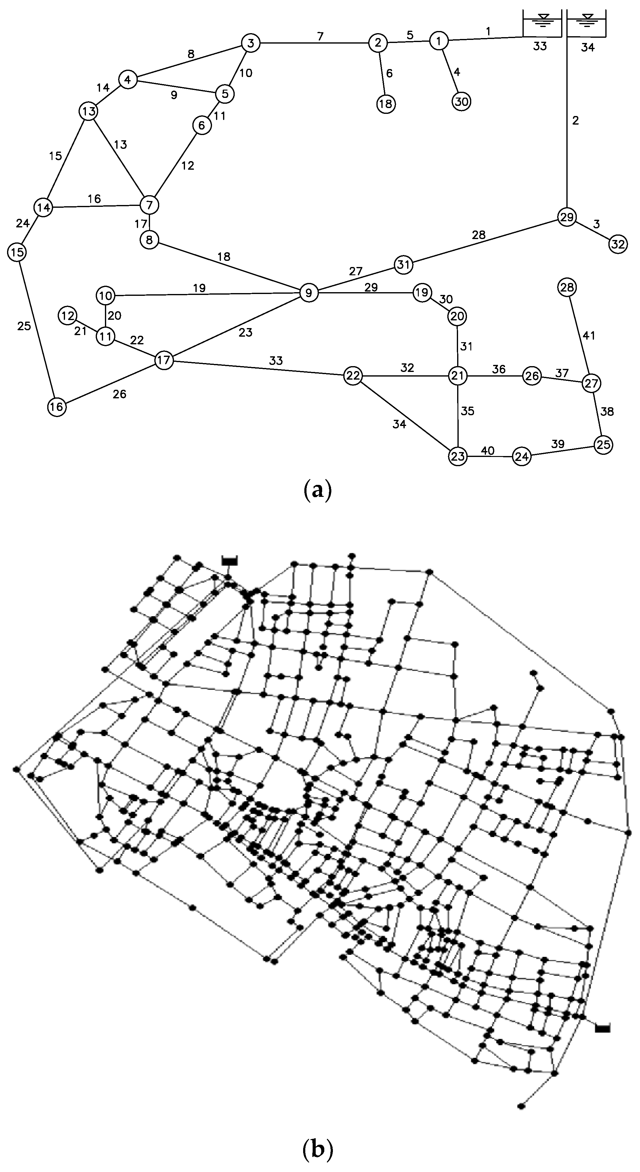
The application of this work concerned two case studies (Figure 2a,b, respectively). The first is the skeletonized WDN of Santa Maria di Licodia, a small town in Sicily, Italy [24,25]. The network layout is made up of 34 nodes (of which 32 are with unknown head and 2 source nodes are with fixed head, i.e., nodes 33 and 34) and of 41 pipes. The features of the WDN nodes and pipes are reported in the referenced work. At the generic demanding node, hmin and hdes were set at 0 and 20 m, respectively.
The two source nodes, i.e., nodes 33 and 34, have a ground elevation of 477.5 m above sea level and a mean daily head of 480.77 m. The topography of the network features declining nodal ground levels as the distance from the source increases. The ground elevation of demanding nodes varies between about 395 and 465 m above sea level.
The whole network demand is 18.5 L/s.
As to leakage, values of the coefficient CL = 2.79 × 10⁻⁸ m0.82/s and of the exponent nleak = 1.18 were assumed for all of the pipes of the network. The values of CL and nleak lead to a daily leakage volume of about 1250 m3, which is about 44% of the water volume leaving the source nodes.
The second case study of the paper is made up of a real WDN in Northern Italy featuring 536 nodes with unknown head, 825 pipes, and 2 reservoirs (Figure 2b) [26]. At the generic demanding node, hmin and hdes were set at 0 and 23 m, respectively. The head of the two reservoirs is 30 m above sea level. Unlike the first network, the second network has flat topography with all nodal ground levels set at 0 m above sea level. The whole network demand is 367 L/s.
As to leakage, values of the coefficient CL = 1.99 × 10⁻⁷ m2.5/s and of the exponent nleak = 0.5 were assumed for all of the pipes of the WDN. The values of CL and nleak lead to a daily leakage volume of about 7920 m3, which is about 20% of the water volume leaving the source nodes.
The two WDNs were solved in snapshot simulations using the five pressure-driven formulations described in Section 2.1. In these simulations, nodal demands were varied considering a uniform multiplying coefficient, αdem, ranging from 1 to 20 with step 1. This resulted in a total framework of 100 simulations (5 pressure driven formulations × 20 demand increase steps) for each WDN. The objective of the simulations was to investigate how differently the pressure-driven formulations react to changes in network operating conditions. In fact, the progressively increasing demand puts the WDNs to an increasingly severe test by lowering nodal pressure heads below hdes and, as a result, by triggering the pressure-driven dependence q(h) (Figure 1). In this analysis, the Wagner et al. [9] formulation was taken as benchmark.
3.2. Results
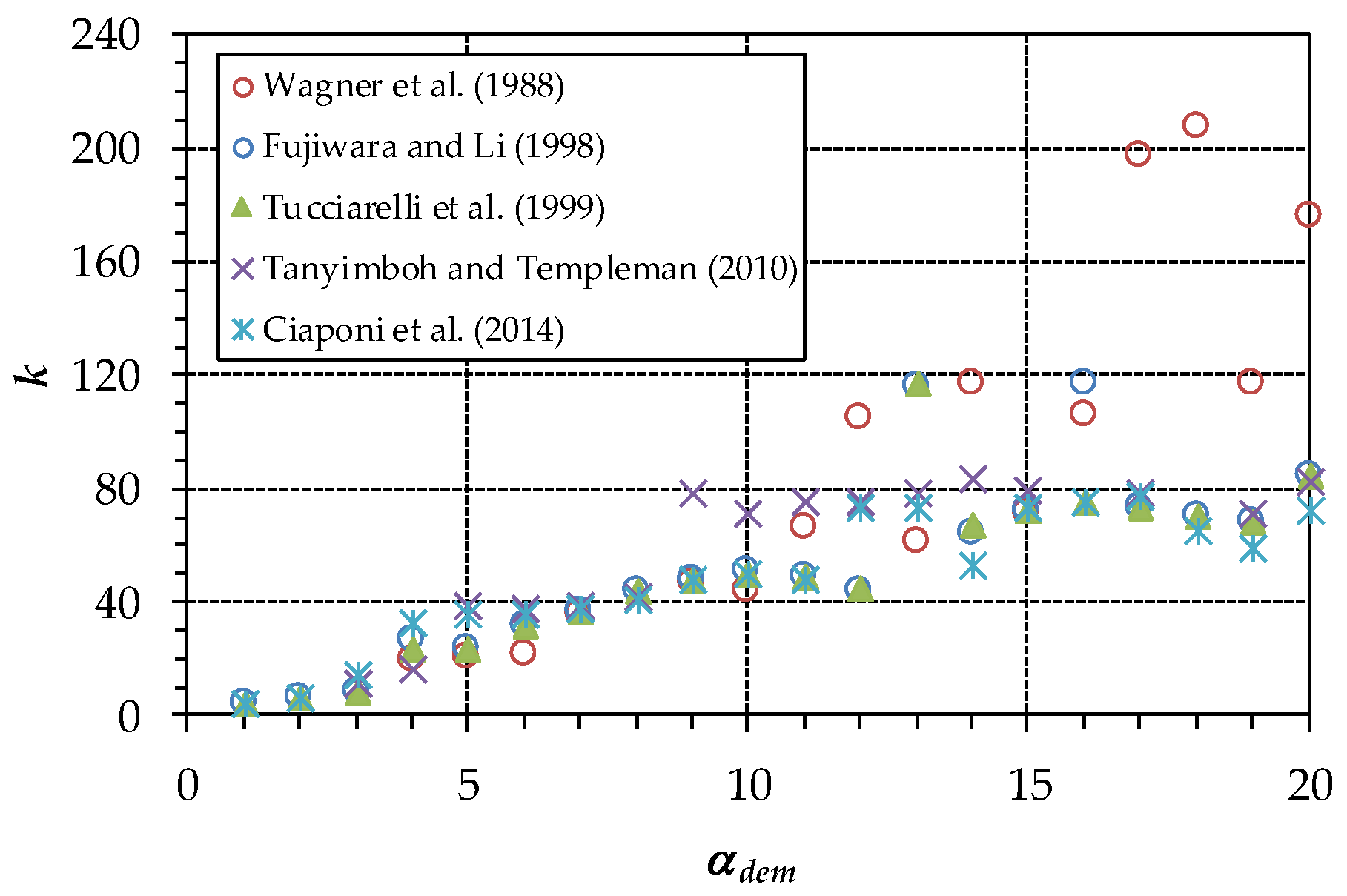
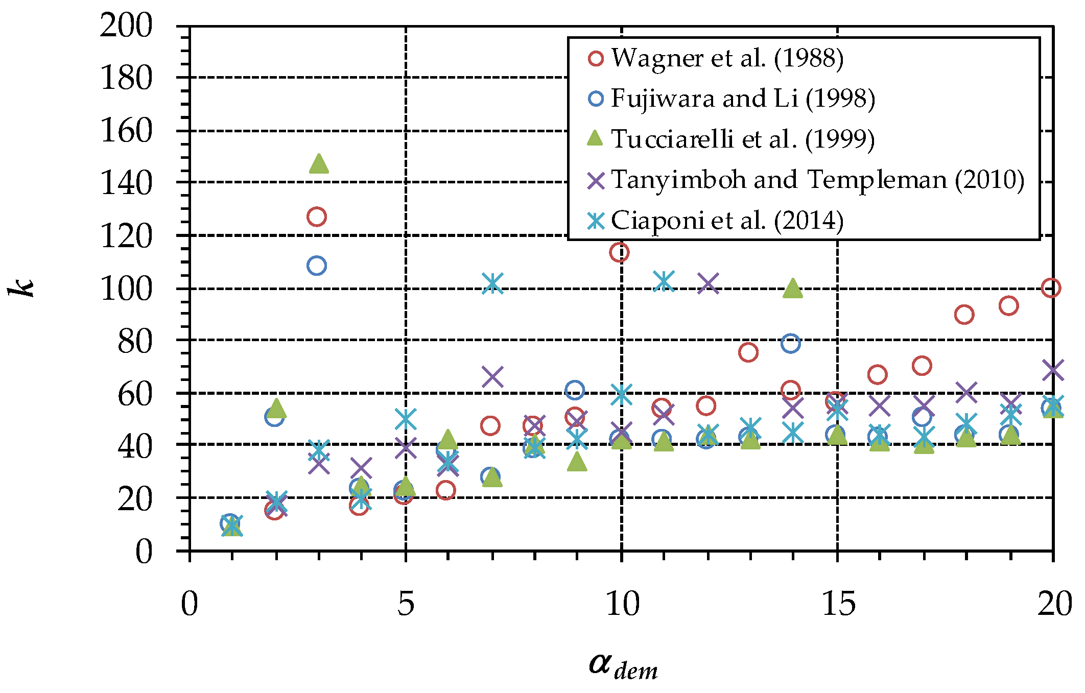
As for the first case study, the first analysis concerns the relationship between the total number k of iterations and αdem (see graph in Figure 3). This graph shows k(αdem) for all of the formulations. For the formulation of Wagner et al. [9], which is the most commonly used in the scientific literature, WDN resolution tends to be slower and slower when αdem grows up to αdem = 20.
The other formulations behave similarly to Wagner et al. [9] up to αdem = 10. Above this value, they tend to converge faster, that is with lower values of k. This seems to suggest that the other formulations suffer from the increase in αdem less than the Wagner et al. [9] formulation.
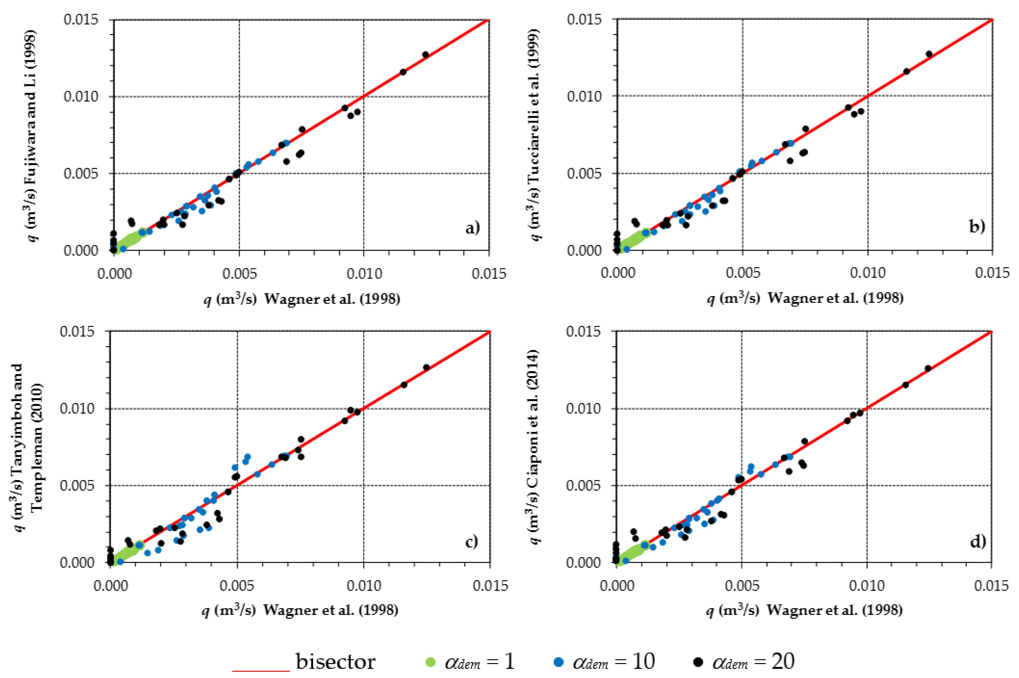
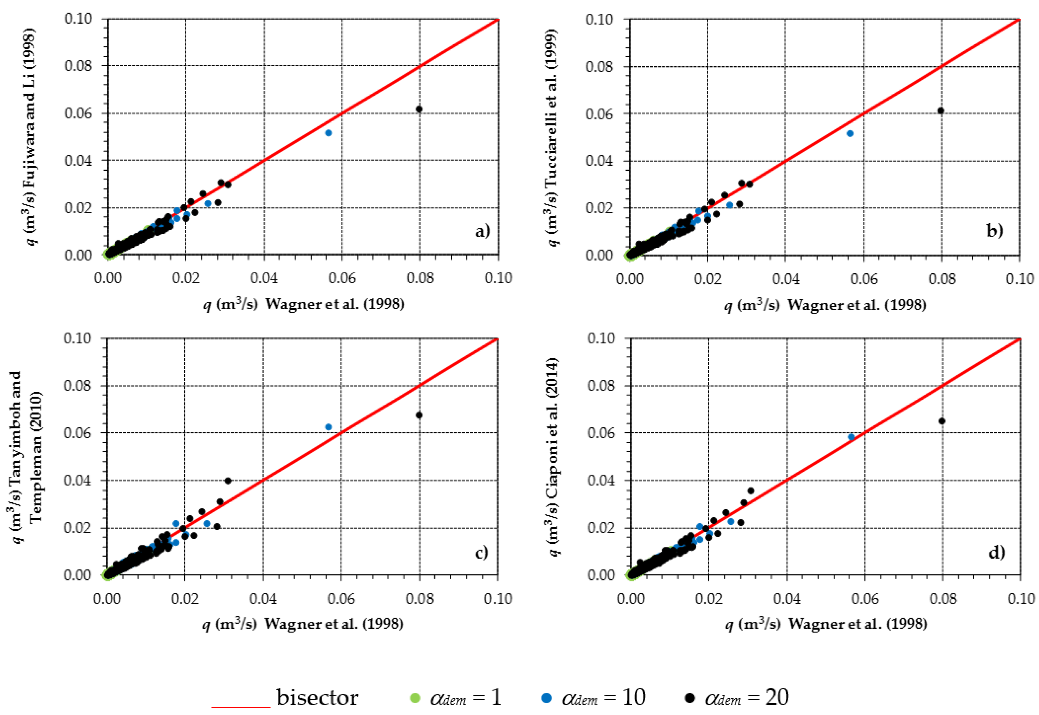
The graphs in Figure 4 and Figure 5 and Table 1 report results concerning analyses and comparisons in terms of outflow q to users. Those in Figure 4 compare the values of q obtained with the Wagner et al. [9] formulation with those obtained with the four other formulations. For αdem = 1, the values are very close because the pressure-driven dependence of q has not been triggered. For larger values of αdem, some differences arise. Far from the 0, the four other formulations yield close values to those of the Wagner et al. [9] formulation, with differences of a similar order of magnitude. However, the differences obtained through the Fujiwara and Li [12] and Tucciarelli et al. [13] formulations are always negative (underestimation). Those obtained through the Tanyimboh and Templeman [17] and of Ciaponi et al. [20] formulations, instead, are alternatively positive and negative. Close to the 0 of the Wagner et al. [9] formulation, all the other formulations tend to yield larger values of q. This behavior may be due to the softer declining trend that the other formulations have in Figure 1 when h/hdes goes down to 0.
A quantitative estimation of the comparison shown in Figure 4 is reported in the following Table 1. This table points out that the mean absolute deviation in q of the various formulations compared to the Wagner et al. [9] formulation tends to grow with αdem. Overall, the formulations yield almost no deviation for αdem = 1, in correspondence to which the pressure-driven behavior is not fully activated. Indeed, it concerns only a few demanding nodes. For αdem = 10 and αdem = 20, they behave similarly, with the Tanyimboh and Templeman [17] and Ciaponi et al. [20] formulations providing the largest deviations, respectively.
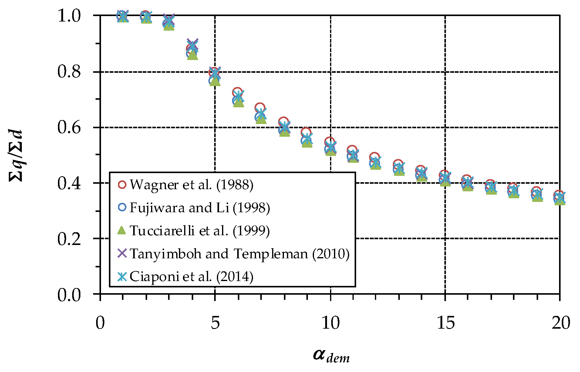
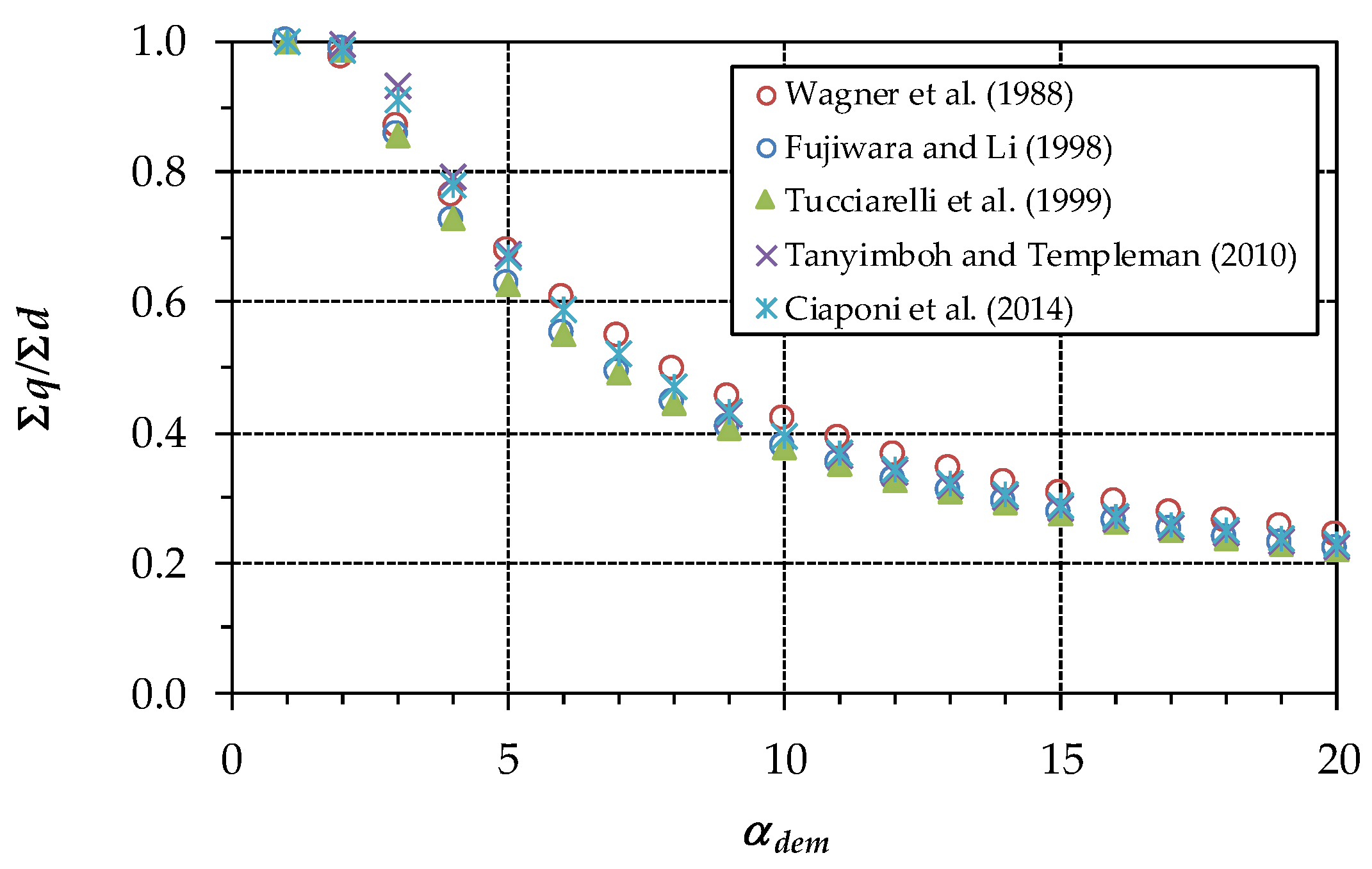
Figure 5 shows the trend of the global demand satisfaction rate ∑q/∑d, as a function of αdem, pointing out that all of the formulations behave similarly. This happens because the overestimations and underestimations compared to the Wagner et al. [9] formulations tend to cancel each other out. As an example of the results, for αdem = 10, the formulations of Fujiwara and Li [12] and of Tucciarelli et al. [13] give a satisfaction rate of 0.52. The Wagner et al. [9] formulation gives a satisfaction rate of 0.55. Finally, the formulations of Tanyimboh and Templeman [17] and of Ciaponi et al. [20] give an intermediate value of 0.53.
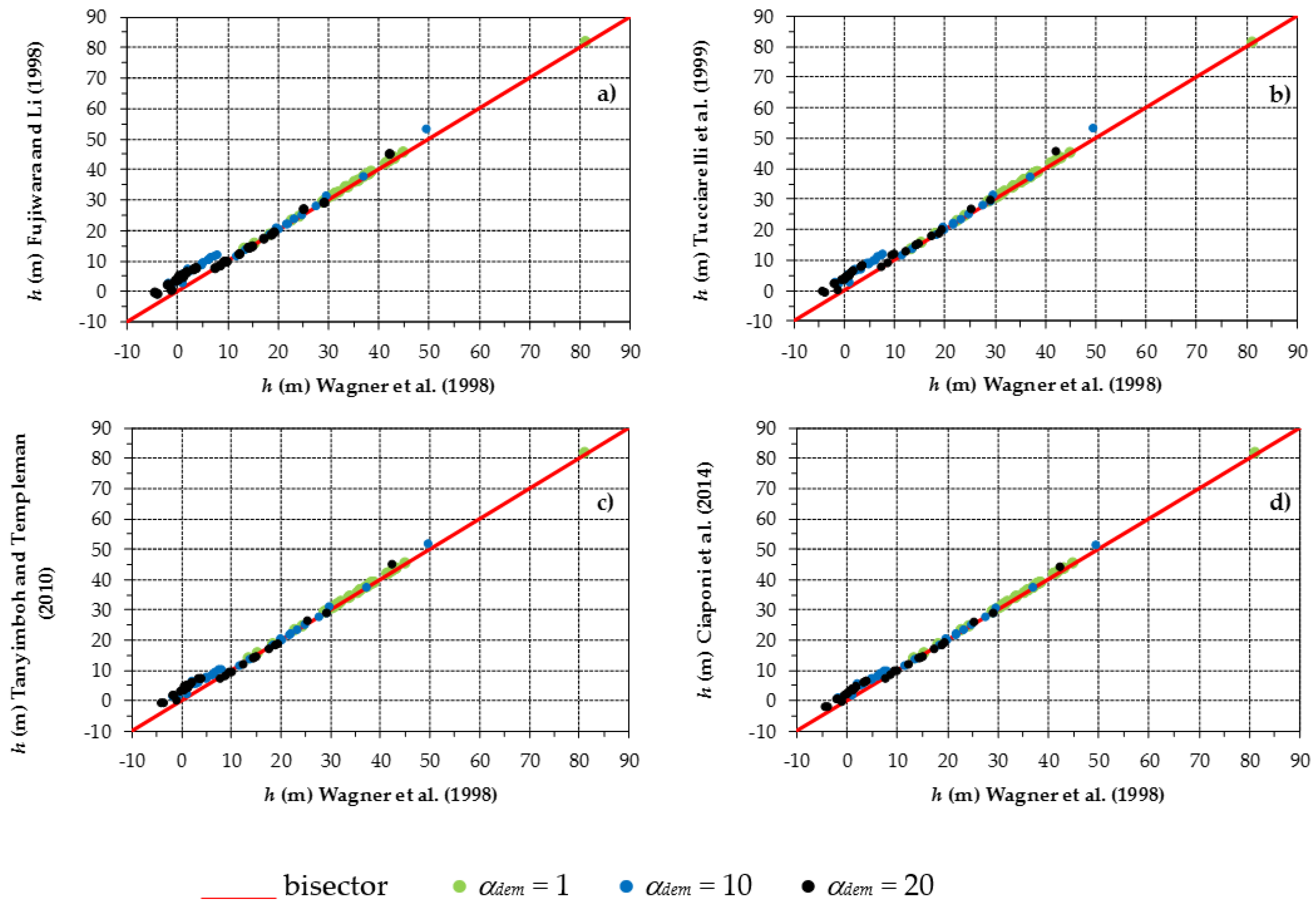
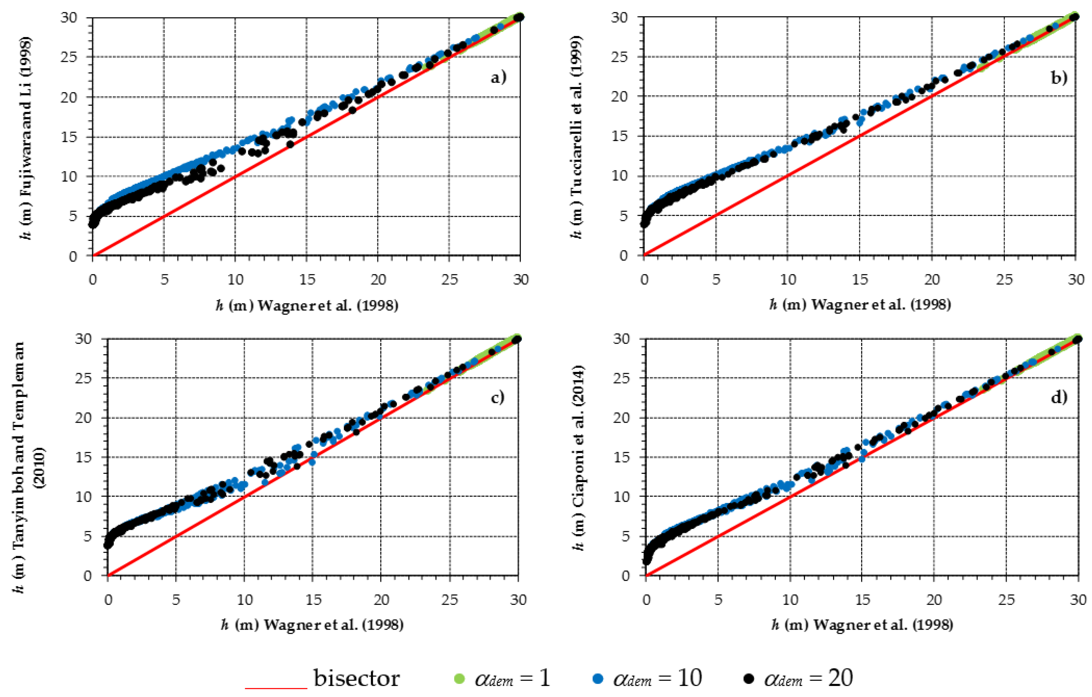
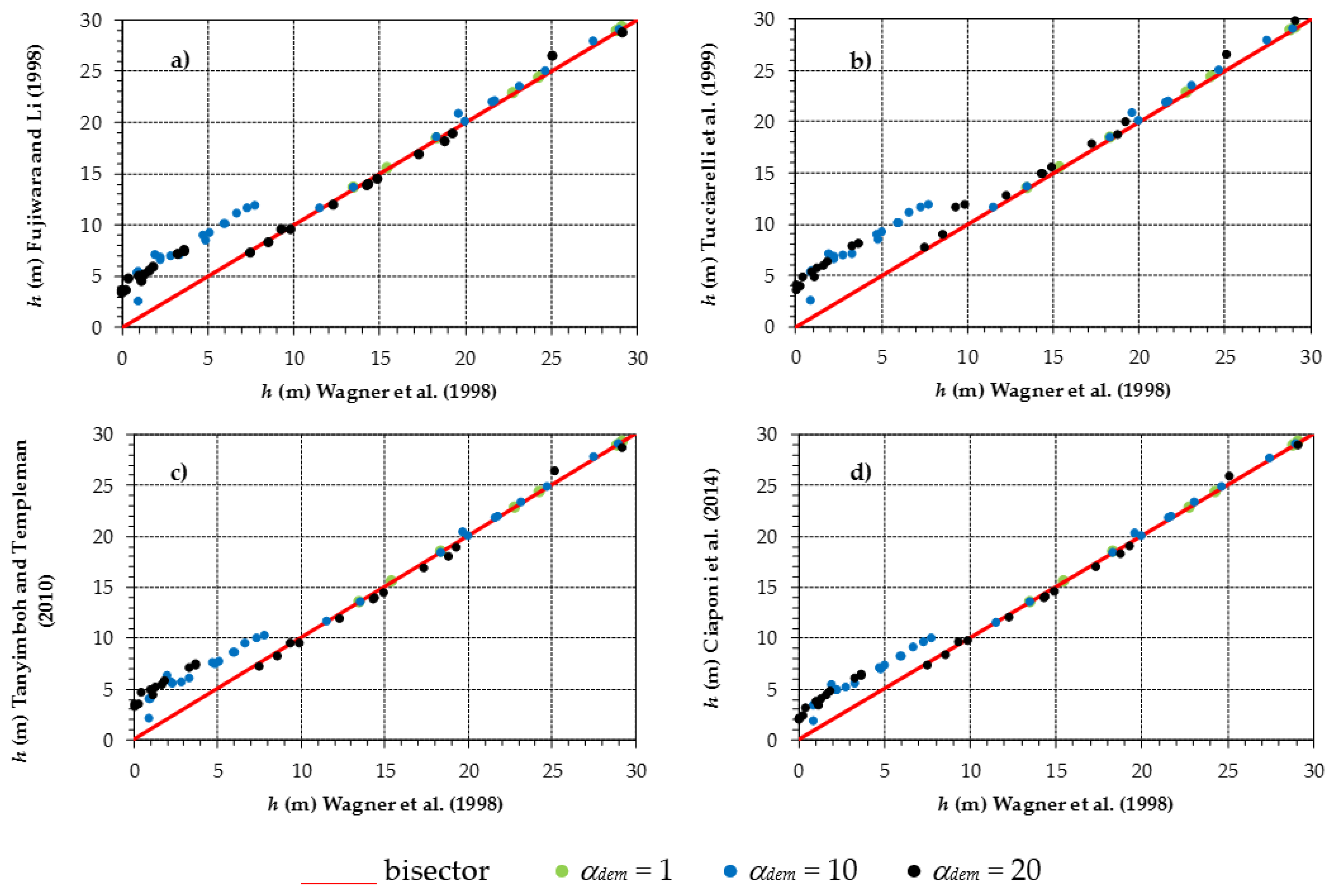
The graphs in Figure 6 compare the nodal pressure heads h obtained with the Fujiwara et al. [12], Tucciarelli et al. [13], Tanyimboh and Templeman [17], and Ciaponi et al. [20] formulations with those obtained with the Wagner et al. [9] formulation. In all cases, the dots are well-aligned along the bisector, apart from close to the 0 of the Wagner et al. formulation, in correspondence to which the other formulations seem to overestimate h.
A quantitative estimation of the comparison shown in Figure 6 is reported in the following Table 2. This table points out that the mean absolute pressure head deviation of the various formulations compared to the Wagner et al. [9] formulation tends to grow with αdem. Overall, the Ciaponi et al. [20] and the Tucciarelli et al. [13] formulations are the closest and furthest, respectively.
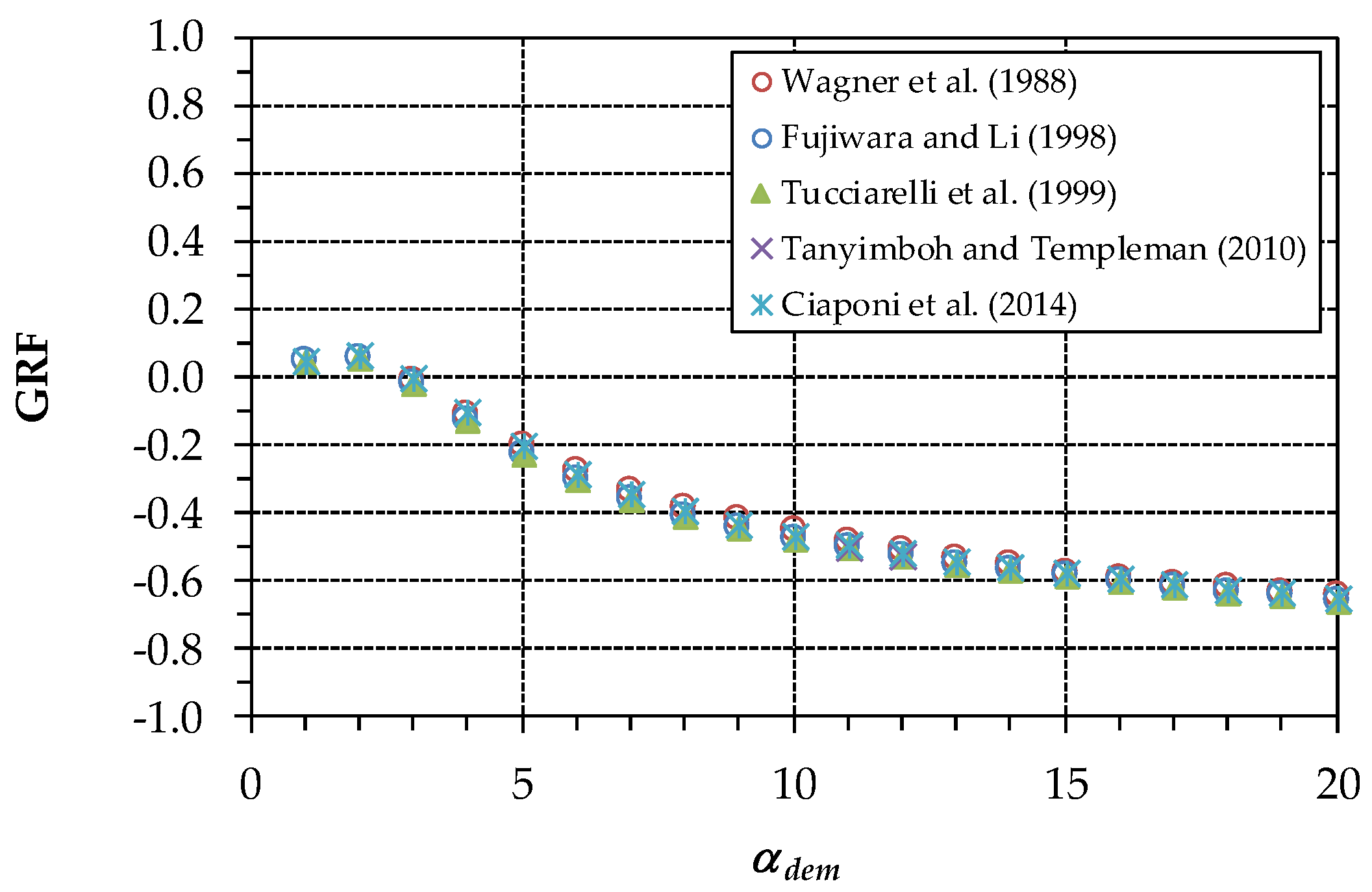
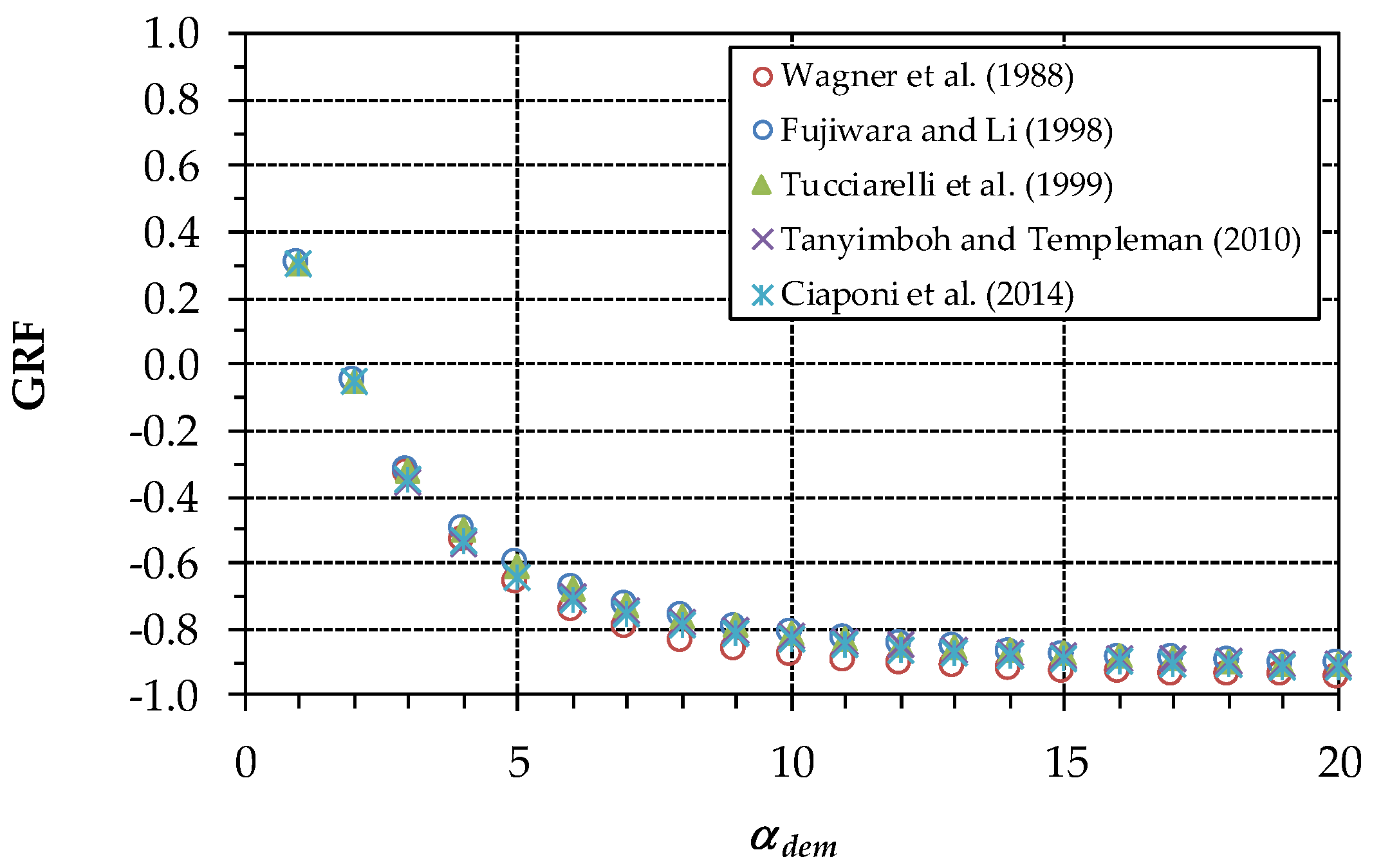
Figure 7 shows the generalized resilience/failure index (GRF) [27] related to the pressure head distribution in the WDN. This index, ranging from −1 to 1, represents an estimate of WDN resilience through the pressure-driven approach when leakage is present. The positive and negative values of GRF are associated with WDNs under power surplus and deficit conditions, respectively. The graph in Figure 7 shows that, despite the differences in h remarked in Figure 6, the formulations yield similar decreasing trends of GRF, as was the case with the satisfaction rate in Figure 5.
The similar values of GRF are because this index depends on both h and q. In fact, the variations in these variables across the various formulations tend to cancel each other out.
The results of the applications to the second case study are reported in the following Figure 8, Figure 9, Figure 10, Figure 11 and Figure 12. These figures are homologous to Figure 3, Figure 4, Figure 5, Figure 6 and Figure 7, respectively, of the first case study. The comparison of Figure 3 and Figure 8 highlights that k tends to grow as αdem grows also for the second case study. However, the beneficial effects of the Fujiwara et al. [12], Tucciarelli et al. [13], Tanyimboh and Templeman [17], and Ciaponi et al. [20] formulations in terms of k reduction, in comparison with the Wagner et al. [9] formulation, are attenuated in the second case study. This may be because of the more interlinked structure of the second network, which helps to regularize pipe flows and nodal heads across the iterations in WDN resolution. All of the other figures have similar interpretations to the homologous figures of the first case study.
The fact that the h overestimation of the Fujiwara et al. [12], Tucciarelli et al. [13], Tanyimboh and Templeman [17], and Ciaponi et al. [20] formulations compared to the Wagner et al. [9] formulation seems to be larger in the second case study (compare Figure 11 with Figure 6) is mainly due to the scale used in the graph (h values ranging from 0 to 30 m in the second case study versus h values ranging from −5 to above 80 m in the first case study). This is clear from Figure 13, where Figure 6 of the first case study is plotted with similar scale to Figure 11.
4. Conclusions
In this paper, a comparison of various pressure-driven formulations, aimed at expressing nodal outflows to users as a function of nodal demands and of the actual nodal pressure, was presented. To this end, the widely adopted formulation of Wagner et al. [9] was taken as benchmark. The comparison was made in the framework of the snapshot steady flow simulation of two different WDNs. These WDNs represent the main skeleton of a poorly interconnected WDN situated in a hilly territory and a very interconnected real WDN situated in a flat territory, respectively. Nodal demands were largely amplified to stress the pressure-driven behavior of the WDNs.
The main outcomes of the work are:
- -
- The increase in nodal demands tends to cause the growth of the number of iterations for WDN algorithm convergence due to the activation of the pressure-driven relationship.
- -
- -
- All formulations similarly simulate nodal outflows.
- -
Though the effects of the various formulations were compared, it must be noted that:
- -
- The different effects of the formulations were accentuated in this work due to the large and uniform amplification of WDN demands. In real cases, the pressure-driven behavior is usually remarkable in small pressure-deficient areas, due to hydrant activations or segment isolations. Therefore, the differences are expected to be more confined.
- -
- Only the comparison with experimental data can reveal which formula is the most consistent with the real WDN behavior.
- -
- In the absence of experimental data, the use of formulations based on statistical simulation of a varied set of situations and phenomena governing the actual water delivery, such as the formulation of Ciaponi et al. [20], may be preferable.
As for the last remarks, it must be noted that parameterizing pressure-driven formulations on the field may be a heavy task. In fact, at a generic WDN node, the outflow q is the only variable that can be measured through metering devices. Demand d can only be supposed. Another tricky factor lies in the fact that, as stated above, the pressure-driven behavior of the WDN is often temporary and unpredictable. Therefore, the only viable option in most circumstances may be the parameterization of the formulations based on statistical simulations of outflow, as was done by Ciaponi et al. [20].
Author Contributions
Both authors contributed equally to the paper.
Conflicts of Interest
The authors declare no conflict of interest.
References
- Wood, D.J.; Charles, O.A. Hydraulic network analysis using linear theory. J. Hydraul. Division 1970, 96, 1221–1234. [Google Scholar]
- Isaacs, L.T.; Mills, K.G. Linear theory methods for pipe network analysis. J. Hydraul. Division 1980, 106, 1191–1201. [Google Scholar]
- Todini, E.; Pilati, S. A Gradient Algorithm for the Analysis of Pipe Networks; Wiley: London, UK, 1988; pp. 1–20. [Google Scholar]
- Creaco, E.; Franchini, M. Comparison of Newton-Raphson Global and Loop Algorithms for Water Distribution Network Resolution. J. Hydraul. Eng. 2014, 140, 313–321. [Google Scholar] [CrossRef]
- Walski, M.; Chase, D.; Savic, D.; Grayman, W.; Beckwith, S.; Koelle, E. Advanced Water Distribution Modelling and Management; Haestad: Waterbury, CT, USA, 2003. [Google Scholar]
- Wu, Z.Y.; Walski, T. Pressure dependent hydraulic modelling for water distribution systems under abnormal conditions. In Proceedings of the IWA World Water Congress and Exhibition, Beijing, China, 10–14 September 2006. [Google Scholar]
- Bhave, P.R. Node flow analysis of water distribution systems. J. Transp. Eng. 1981, 107, 457–467. [Google Scholar]
- Germanopoulos, G. A technical note on the inclusion of pressure dependent demand and leakage terms in water supply network models. J. Civ. Eng. Syst. 1985, 2, 171–179. [Google Scholar] [CrossRef]
- Wagner, B.J.M.; Shamir, U.; Marks, D.H. Water distribution reliability: Simulation method. J. Water Resour. Plan. Manag. 1988, 276–294. [Google Scholar] [CrossRef]
- Chandapillai, J. Realistic simulation of water distribution system. J. Transp. Eng. 1991, 258–263. [Google Scholar] [CrossRef]
- Gupta, R.; Bhave, P.R. Comparison of methods for predicting deficient-network performance. J. Water Resour. Plan. Manag. 1996, 214–217. [Google Scholar] [CrossRef]
- Fujiwara, O.; Li, J. Reliability analysis of water distribution networks in consideration of equity, redistribution, and pressuredependent demand. J. Water Resour. Res. 1998, 34, 1843–1850. [Google Scholar] [CrossRef]
- Tucciarelli, T.; Criminisi, A.; Termini, D. Leak Analysis in Pipeline System by Means of Optimal Value Regulation. J. Hydraul. Eng. 1999, 125, 277–285. [Google Scholar] [CrossRef]
- Alvisi, S.; Franchini, M. Near-optimal rehabilitation scheduling of water distribution systems based on a multi-objective genetic algorithm. Civ. Eng. Environ. Syst. 2006, 23, 143–160. [Google Scholar] [CrossRef]
- Giustolisi, O.; Savic, D.; Kapelan, Z. Pressure-driven demand and leakage simulation for water distribution networks. J. Hydraul. Eng. 2008, 626–635. [Google Scholar] [CrossRef]
- Wu, Z.Y.; Wang, R.H.; Walski, T.M.; Yang, S.Y.; Bowdler, D.; Baggett, C.C. Extended global-gradient algorithm for pressure-dependent water distribution analysis. J. Water Resour. Plan. Manag. 2009. [Google Scholar] [CrossRef]
- Tanyimboh, T.; Templeman, A. Seamless pressure-deficient water distribution system model. J. Water Manag. 2010, 163, 389–396. [Google Scholar] [CrossRef] [Green Version]
- Creaco, E.; Franchini, M.; Alvisi, S. Evaluating water demand shortfalls in segment analysis. Water Resour. Manag. 2012, 26, 2301–2321. [Google Scholar] [CrossRef]
- Siew, C.; Tanyimboh, T.T. Pressure-dependent EPANET extension. J. Water Resour. Manag. 2012, 26, 1477–1498. [Google Scholar] [CrossRef] [Green Version]
- Ciaponi, C.; Franchioli, L.; Murari, E.; Papiri, S. Procedure for defining a pressure-outflow relationship regarding indoor demands in pressure-driven analysis of water distribution networks. Water Resour. Manag. 2015, 29, 817–832. [Google Scholar] [CrossRef]
- Elhay, S.; Piller, O.; Deuerlein, J.; Simpson, A. A robust, rapidly convergent method that solves the water distribution equations for pressure-dependent models. J. Water Resour. Plan. Manag. 2015, 04015047. [Google Scholar] [CrossRef]
- Pacchin, E.; Alvisi, S.; Franchini, M. Analysis of Non-Iterative Methods and Proposal of a New One for Pressure-Driven Snapshot Simulations with EPANET. Water Resour. Manag. 2017, 31, 75–91. [Google Scholar] [CrossRef]
- Todini, E.; Rossman, L.A. Unified framework for deriving simultaneous equation algorithms for water distribution networks. J. Hydraul. Eng. 2013, 139, 511–526. [Google Scholar] [CrossRef]
- Pezzinga, G. Procedure per la riduzione delle perdite mediante il controllo delle pressioni. In Ricerca e Controllo delle Perdite Nelle Reti di Condotte. Manuale per una Moderna Gestione degli Acquedotti; Brunone, B., Ferrante, M., Meniconi, S., Eds.; CittàStudiEdizioni: Novara, Italy, 2008. (In Italian) [Google Scholar]
- Creaco, E.; Pezzinga, G. Embedding Linear Programming in Multi Objective Genetic Algorithms for Reducing the Size of the Search Space with Application to Leakage Minimization in Water Distribution Networks. Environ. Model. Softw. 2015, 69, 308–318. [Google Scholar] [CrossRef]
- Creaco, E.; Franchini, M. Fast network multi-objective design algorithm combined with an a posteriori procedure for reliability evaluation under various operational scenarios. Urban Water J. 2012, 9, 385–399. [Google Scholar] [CrossRef]
- Creaco, E.; Franchini, M.; Todini, E. Generalized Resilience and Failure Indices for Use with Pressure-Driven Modeling and Leakage. J. Water Resour. Plan. Manag. 2017, 142, 04016019. [Google Scholar] [CrossRef]
Figure 1.
Ratio of outflow q to demand d as a function of the ratio of the generic pressure head h to the desired pressure head hdes for the various formulations.
Figure 1.
Ratio of outflow q to demand d as a function of the ratio of the generic pressure head h to the desired pressure head hdes for the various formulations.

Figure 2.
Water distribution networks (WDNs) for the two case studies (a,b). In the first case study with source nodes 33 and 34, pipe numbers are close to the pipes and the numbers of demanding nodes are inside circles.
Figure 2.
Water distribution networks (WDNs) for the two case studies (a,b). In the first case study with source nodes 33 and 34, pipe numbers are close to the pipes and the numbers of demanding nodes are inside circles.

Figure 3.
First case study. Number k of iterations as a function of αdem for the various formulations.
Figure 3.
First case study. Number k of iterations as a function of αdem for the various formulations.

Figure 4.
First case study. Comparison of the various formulations, (a) Fujiwara and Li [12], (b) Tucciarelli et al. [13], (c) Tanyimboh and Templeman [17] and (d) Ciaponi et al. [20], in terms of outflow q to users.

Figure 5.
First case study. Satisfaction rate ∑q/∑d for the various formulations as a function of αdem.
Figure 5.
First case study. Satisfaction rate ∑q/∑d for the various formulations as a function of αdem.

Figure 6.
First case study. Comparison of the various formulations, (a) Fujiwara and Li [12], (b) Tucciarelli et al. [13], (c) Tanyimboh and Templeman [17] and (d) Ciaponi et al. [20], in terms of nodal pressure head h.

Figure 7.
First case study. Generalized resilience/failure index (GRF) for the various formulations as a function of αdem.
Figure 7.
First case study. Generalized resilience/failure index (GRF) for the various formulations as a function of αdem.

Figure 8.
Second case study. Number k of iterations as a function of αdem for the various formulations.
Figure 8.
Second case study. Number k of iterations as a function of αdem for the various formulations.

Figure 9.
Second case study. Comparison of the various formulations, (a) Fujiwara and Li [12], (b) Tucciarelli et al. [13], (c) Tanyimboh and Templeman [17] and (d) Ciaponi et al. [20], in terms of outflow q to users.

Figure 10.
Second case study. Satisfaction rate ∑q/∑d for the various formulations as a function of αdem.
Figure 10.
Second case study. Satisfaction rate ∑q/∑d for the various formulations as a function of αdem.

Figure 11.
Second case study. Comparison of the various formulations, (a) Fujiwara and Li [12], (b) Tucciarelli et al. [13], (c) Tanyimboh and Templeman [17] and (d) Ciaponi et al. [20], in terms of nodal pressure head h.

Figure 12.
Second case study. GRF for the various formulations as a function of αdem.

Figure 13.
First case study. Comparison of the various formulations, (a) Fujiwara and Li [12], (b) Tucciarelli et al. [13], (c) Tanyimboh and Templeman [17] and (d) Ciaponi et al. [20], in terms of nodal pressure head h. Zoom of Figure 6 with scale similar to Figure 11.


Table 1.
First case study. Mean absolute deviation (m3/s) of the various formulations in terms of outflow q to users compared to the Wagner et al. [9] formulation for the three values of αdem.
Table 1.
First case study. Mean absolute deviation (m3/s) of the various formulations in terms of outflow q to users compared to the Wagner et al. [9] formulation for the three values of αdem.
| Formulation | αdem = 1 | αdem = 10 | αdem = 20 |
|---|---|---|---|
| Fujiwara and Li [12] | 0 | 0.00022 | 0.00049 |
| Tucciarelli et al. [13] | 0 | 0.00024 | 0.00049 |
| Tanyimboh and Templeman [17] | 0 | 0.00042 | 0.00044 |
| Ciaponi et al. [20] | 0 | 0.00029 | 0.00051 |
Table 2.
First case study. Mean absolute deviation (m) of the various formulations in terms of nodal pressure head h compared to the Wagner et al. [9] formulation for the three values of αdem.
Table 2.
First case study. Mean absolute deviation (m) of the various formulations in terms of nodal pressure head h compared to the Wagner et al. [9] formulation for the three values of αdem.
| Formulation | αdem = 1 | αdem = 10 | αdem = 20 |
|---|---|---|---|
| Fujiwara and Li [12] | 0.0012 | 2.65 | 2.69 |
| Tucciarelli et al. [13] | 0.0010 | 2.68 | 2.76 |
| Tanyimboh and Templeman [17] | 0.0024 | 1.84 | 2.26 |
| Ciaponi et al. [20] | 0.0013 | 1.54 | 1.54 |
© 2018 by the authors. Licensee MDPI, Basel, Switzerland. This article is an open access article distributed under the terms and conditions of the Creative Commons Attribution (CC BY) license (http://creativecommons.org/licenses/by/4.0/).
Share and Cite
MDPI and ACS Style
Ciaponi, C.; Creaco, E. Comparison of Pressure-Driven Formulations for WDN Simulation. Water 2018, 10, 523. https://doi.org/10.3390/w10040523
AMA Style
Ciaponi C, Creaco E. Comparison of Pressure-Driven Formulations for WDN Simulation. Water. 2018; 10(4):523. https://doi.org/10.3390/w10040523
Chicago/Turabian StyleCiaponi, Carlo, and Enrico Creaco. 2018. "Comparison of Pressure-Driven Formulations for WDN Simulation" Water 10, no. 4: 523. https://doi.org/10.3390/w10040523
Note that from the first issue of 2016, this journal uses article numbers instead of page numbers. See further details here.