Abstract
In this study, an inexact two-stage stochastic programming (ITSP) model was developed for supporting water resources allocation for the four main water use sectors (industry, municipal, environmental, and agriculture) and total amount control of the pollutant emissions. The Yinma River Basin in northeast China was selected for a case study. A number of scenarios corresponding to different flow levels were examined. The flow levels reflect different probabilities of water resource availability and environmental carrying capacity. The results revealed that the optimal allocation strategies for each sector depend on water resource carrying capacity, wastewater treatment capacity, the total amount of regional control, and the water environment carrying capacity. Water ecology projects were identified that are needed to treat contaminated water and to address the insufficient carrying capacity for pollutant emissions generated in water-using processes. The results will be helpful for establishing sensible water management systems that integrate the development and utilization of water resources and protect the environment, and for providing a basis for water pollution prevention plans, the model can be used to guide management interventions to improve the water environment by regional pollutant emission control and the improvement of carrying capacity in the Yinma River Basin.
1. Introduction
Water resources play an essential role in human survival, sustainable socioeconomic development, and the eco-environment [1]. However, as a result of rapid population growth and socioeconomic development, excessive exploitation of water causes severe shortages of water resources and the destruction of water ecosystems, especially in water-stressed areas [2,3]. At the same time, wastewater discharge leads to the deterioration of the water environment quality, creating further water resource problems [4,5]. In addition, there are many uncertainties in the water environment system, such as the variability in the availability of water resources, variability in the development of technology, variability of demand, and the complexity of the interconnected processes (e.g., water utilization, recycling, wastewater treatment, and discharge) [6]. In practice, these uncertainties generate enormous challenges for water resources allocation and water quality management. Therefore, effective optimization approaches to water management in complex, uncertain conditions are necessary. Water management issues that need to be optimized include water resources allocation and utilization, water quality management, environmental protection, and regional development.
Previously, a number of optimization approaches (e.g., interval-parameter programming, fuzzy programming, and stochastic programming) were developed for water resources allocation and water quality management under uncertainty [7,8,9,10,11,12,13,14]. Among these approaches, the inexact two-stage stochastic programming (ITSP) model, which integrates the interval-parameter programming (IPP) and two-stage stochastic programming (TSP), could reduce uncertainties to discrete interval-parameters and probability distributions [15]. ITSP has been widely applied for dealing with different forms of multiple uncertainties in water resource allocation and water quality management [15]. For example, Maqsood [16] presented an interval-parameter, fuzzy, two-stage stochastic programming (IFTSP) method for the planning of water resource management systems under uncertainty; Xu [17] developed an inexact, two-stage, stochastic, robust programming model for dealing with water resources allocation problems under uncertainty. Xie [18] developed an inexact, two-stage, water resources management model for multi-regional water resources planning in the Nansihu Lake Basin, China. In ITSP, an initial decision is made before the random events. After the future uncertainties are resolved and the values of the random variables are known, a second decision is made that minimizes penalties caused by any infeasibilities [15].
Thus, it can be seen that ITSP is a suitable and effective approach for water resources allocation and water quality management under uncertainty [19,20,21,22]. However, previous studies always focus on water resource allocation and water quality management based on ideal water environmental carrying capacity, seldom considered the water quality management of contaminated rivers, especially severely contaminated water bodies such as the Yinma River that have a large imbalance between environmental carrying capacity and pollutant emissions [23]. In 2014, the total amounts of chemical oxygen demand (COD) and NH4-N discharged into the Yinma River were 33.29 × 10³ tons and 3.60 × 10³ tons, respectively, far in excess of the water environment carrying capacities of 13.55 × 10³ tons and 0.52 × 10³ tons, respectively. Due to constraint of the regional development requirement, considering pollutant emission reduction only would be difficult and unlikely to achieve the objectives of water quality improvement and restoration [24]. The improvement of the water environment carrying capacity should be considered in water quality management. Water ecological restoration projects, such as constructed wetlands, ecological floating beds, dredging engineering, and artificial aeration, have been demonstrated to be efficient for improving water environment quality and carrying capacity [25,26,27,28], but are rarely considered in water quality management models. Furthermore, the global water resources availability is decreasing [29]; climate change has shown non-linear and non-stationary impacts on different water resources (e.g., blue water and green water flow and storage) [30,31,32], sediment [33,34,35,36], water quality [37,38,39], etc. Hence, there is a need to better optimize the available water resources of the world in general, and the Yinma River Basin, in particular. The Yinma River Basin has a semi-humid climate, with a mean annual precipitation of 580 mm, and a drought index of about 1.0–2.6. Water resource shortages are common in this area. The water resources have a greater than 70% utilization rate, and the water resource per capita is 378 m3, which is 18% of the national average [40]. Moreover, as a result of over-exploitation, the Yinma River experiences increasing environmental problems, such as serious water pollution and ecological damage. It has been documented that the majority of the river does not meet water quality targets. More than 80% of the Yinma River has a contaminated status, especially in the downstream sections, and concentration indexes of the main pollutants at monitored sections are Grade V or worse in terms of the national quality standards. It would be unrealistic to deal with these problems solely by enhancing water use efficiency and reducing pollutant discharge.
Therefore, to add to the previous studies, this study has the objective of developing an ITSP model for water management in the Yinma River Basin that integrates water resources allocation, water equality management, and ecological restoration projects, to deal with the optimal water resources allocation for water-using departments, and the balance between water utilization and pollutant emissions, total amount control, and water environmental carrying capacity which should be improved by ecological restoration projects. Figure 1 presents the general framework of the ITSP model for water management in the Yinma River Basin under uncertainty for integrating water quality management and water resources allocation. The modeling results could help allocate water resource quantities to different water use sectors and help generate rational pollutant emission schemes and cost-effective ecological restoration projects. Thus, the results could be of value for supporting local decision-makers in generating regional water resources utilization and water pollution control schemes that are consistent with sustainable economic-environmental development.
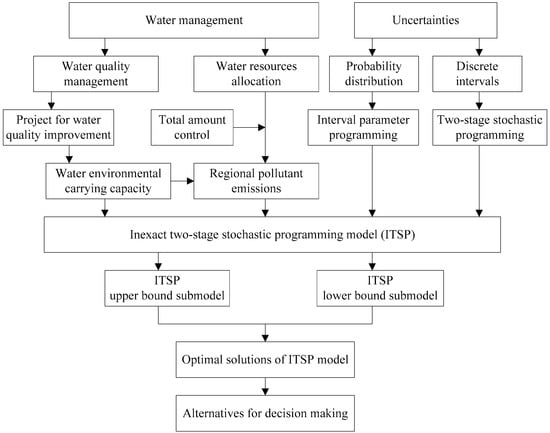
Figure 1.
Framework for the inexact two-stage stochastic programming (ITSP) model.
2. Study Area
The Yinma River (43°14′–44°53′ N, 125°30′–126°15′ E) is located in the central part of Jilin Province, China. The river originates in Panshi County and flows through Shuangyang District, Yongji County, Jiutai District, and Dehui City, before flowing into the Second Songhua River, after the junction with the Yitong River in Nong’an County. The river has a total length of 387.5 km, and the Yinma River Basin has an area of more than 8056 km2 (this does not include the Yitong River) [41].
In this study, in order to clearly reflect different water environmental functions, and relationships between water utilization, pollutants generation, and discharge directions, the Yinma River Basin was divided into 11 water environment zones (i = 1–11 represent I, II, III, IV, V, VI, VII, VIII, IX, X, and XI) and eight administrative regions (j = 1–8 represent Panshi, Yongji, Shuangyang, Jiutai, Dehui, Yitong, Changchun, and Nongan). The zones and regions are shown in Figure 2. Table 1 lists the relationships between regional pollutant emissions and receiving water, including pollutant emission directions and proportions. The values show the proportion of pollutant emissions generated from region j and discharged into the water environment zone i.
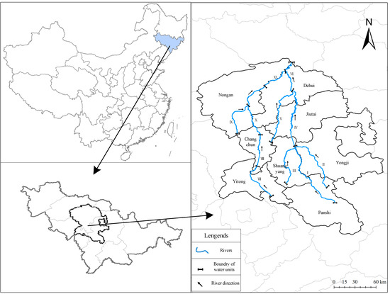
Figure 2.
Geographical position and study regions of the Yinma River Basin.

Table 1.
Relationships between regional pollutant emission and receiving water.
3. Model Formulation
3.1. Model Development
This study considers long-run programming. The planning horizon covers 15 years with five years per period (i.e., 2016–2020, 2021–2025, and 2026–2030), and has three scenarios for flow levels (low, medium, and high), reflecting different probabilities of available water resources and water environmental carrying capacities. The applicability of the engineering improvements differed in different water environment zones and necessitated an adjustment in the initial allocation of water resources, to balance pollutants amount discharged into the rivers and water environmental carrying capacities. The ITSP method is considered suitable for addressing the local issues. The inexact, two-stage, stochastic programming model for integrating engineering technologies and water resources allocation in the Yinma River Basin can be formulated as follows:
where is the total expected system benefit (104 RMB) over the planning periods.
(1) Water utilization benefits
where denotes the controlling administrative region; denotes the water use sectors ( = 1 for industry, = 2 for municipal, = 3 for the environment, and = 4 for agriculture); t denotes different periods in the planning horizon (t = 1 is 2016–2020, t = 2 is 2021–2025, and t = 3 is 2026–2030); denotes length of period t, and the values are fixed at 5 years; represents water-use benefit for each sector k in region j (104 RMB/104 m3); represents pre-allocation of water resources for sector k during period t in region j (104 m3/year); and represents reused water resources for sector k during period t in region j (104 m3/year).
(2) Water shortage penalty
where h denotes various scenarios of runoff in every period (h = 1, 2, and 3 for low, medium, and high levels, respectively); denotes the occurrence probability of scenario h; represents the reduction of net benefit to sector k per unit of water resource not delivered (104 RMB/104 m3); and represents the allocation deficit of water resources for sector k during period t in region j under scenario h (104 m3/year).
(3) Water supply cost
where represents the costs of water supply of sector k during period t in region j (104 RMB/104 m3); and is the cost of reused water supply for sector k during period t in region j (104 RMB/104 m3).
(4) Wastewater treatment cost
where represents the costs of wastewater treatment for sector k during period t in region j (104 RMB/104 m3); denotes the costs of wastewater reclamation for sector k during period t in region j (104 RMB/104 m3).
(5) Environmental capacity improvement cost
where i is the water environment zone; l is the engineering required for carrying capacity improvement (l = 1, 2, 3, 4, 5, 6, and 7 are wetland, ecological floating bed, ecological corridor, pre-tank construction, conservation forest, dredging engineering, and artificial aeration, respectively); is the quantity of engineering l in zone i during period t; is the cost of engineering l in zone i.
Constraints:
(1) Water supply constraints
where denotes available water resources under scenario h during period t (104 m3/year).
(2) Demand constraints of water use sectors
where represents the minimum water resources requirement of sector k during period t in region j (104 m3/year); and represents the maximum water resources requirement of sector k during period t in region j (104 m3/year).
(3) Regional wastewater treatment capacity constraints
where is the wastewater emission coefficient for sector k during period t in region j; is the wastewater concentration treatment coefficient for sector k during period t in region j; and represents the wastewater treatment capacity of sector k during period t in region j (104 tons).
(4) Regional wastewater reuse capacity constraints
where is the wastewater reuse rate of sector k during period t in region j.
(5) Constraints for the total emissions of water pollutants
where r is the controlled water pollutant (r = 1 for chemical oxygen demand (COD), r = 2 for ammonia nitrogen (NH4-N)); represents the concentration of pollutant r after wastewater treatment by sector k during period t (mg/L); represents the concentration of pollutant r without treatment from sector k during period t (mg/L); and represents the total amount of pollutant r during period t in region j (tons).
(6) Water environment carrying capacity constraint
where represents the river load ratio of pollutant r from sector k during period t; is the receiving ratio of water zone i from region j; is the improvement in the carrying capacity for pollutant r by engineering l in zone i during period t; is the maximum quantity constraint for engineering l in zone i during period t; and is the carrying capacity (tons) of pollutant r in zone i during period t under scenario h.
(7) Engineering constraints for carrying capacity improvement
(8) Other
The objective is to maximize the total system benefit in the river basin, which includes the related benefit from the water use sectors under the pre-allocation of water resources; the penalties when the permitted allocation is not delivered; and the cost of water supply, wastewater treatment, wastewater reclamation, and engineering to improve the water environment carrying capacity. The constraints are for the relationships between decision values and water quality requirements, including the available water resources, regional total amount controlled, water carrying capacity, and ecological engineering.
Using an interactive algorithm, the ITSP model can be transformed into two deterministic sub-models that correspond to the lower and upper bounds of the desired objective function value. By solving the two sub-models, , , and , , were obtained and formed the final solution of the ITSP model as [, ], [, ], and [, ].
3.2. Parameters
Table 2 lists the initial water resources allocation strategies in the Yinma River Basin; these were determined based on the latest 10 years of regional water resource consumption in each sector and on development planning for the river basin.

Table 2.
Initial water resource allocation in the Yinma River Basin (104 m3/year).
4. Results Analysis and Discussion
4.1. Water Resource Allocation
Table 3 lists the optimal water resources pre-allocation for the Yinma River Basin. The table indicates that the optimal allocation is close to the lower boundary of the initial water resource allocation—a result of the higher water shortage probability, and because a lower pre-allocation would be more reasonable for different water use sectors and would lead to lower penalties caused by water resource deficits [22].

Table 3.
Optimal water resource pre-allocations for the Yinma River Basin (104 m3/year).
Figure 3, Figure 4 and Figure 5 show the reused water allocation for the industrial, municipal, and environment sectors. Figure 3 indicates different tendencies for reused water allocation for industry in the three periods. In Regions 2, 4, and 8 the allocations of reused water increase gradually over time because of higher water consumption and reuse rates. For example, in Region 2, the amounts were 951 × 104, 1085 × 104, and 1225 × 104 m3/year in three periods. However, in Regions 1 and 7, the amounts of reused water show an opposite trend; the values are 368.8 × 10⁴, [237.3, 297.2] × 104, [20.1, 220.7] × 104 m3/year, and 1022 × 104 m3/year, 0, and 0, in three periods, respectively. There are two reasons for this trend: (1) the water resources pre-allocation was obtained that was close to the maximum water resource requirements; and (2) more water consumption results in more wastewater generation, which would be constrained by wastewater treatment capacity. For these reasons, higher pre-allocations of water resources might lead to wasting of water resources. Figure 4 and Figure 5 show reused water allocations for the municipal and environment sectors, all of which were generated by the municipal sector. From these figures, it can be seen the amount of the reused water allocation for the two sectors has clear differences. The amount of reused water allocated to the environment sector increased gradually over time, which is the opposite of the municipal sector. For example, in Region 1, the amounts of reused water allocated to the environment sector are [54.3, 324.0] × 104, [209.1, 375.2] × 104, and [316.7, 414.7] × 104 m3/year in the three periods, while for the municipal sector the amounts are [0, 229.2] × 104, [0, 119.2] × 104, and [0, 46.2] × 104 m3/year, respectively. The main reason for this trend is that the environment sector generates more benefits through water consumption and has a higher water requirement; when the water resource allocation meets the minimum water resource requirement, more reused water was allocated to the environment sector.
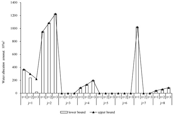
Figure 3.
Reused water resource allocations for industry.
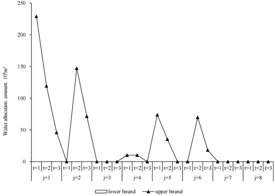
Figure 4.
Reused water resource allocations for municipal use.
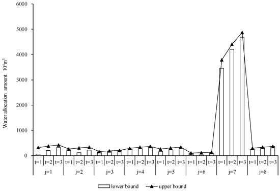
Figure 5.
Reused water resource allocations for the environment.
Table 4, Table 5 and Table 6 list the water resources deficit for each sector under different scenarios in the three periods. From these tables, it can be clearly seen that the deficit decreases as the available water resources increase (h = 1, 2, 3). For example, in Period 1, Region 7, there were no deficits in the industrial sector, and the deficits in the other sectors were [3707.80, 5014.09] × 104, [0.00, 5014.09] × 104, and 0.00 m3/year in the municipal sector; [0.00, 349.83] × 104 m3/year, 0.00, and 0.00 in the environment sector; and [7394.40, 8521.60] × 104, [0.00, 8521.60] × 104, and 0.00 m3/year in agricultural sector department. In general, except in Regions 5 and 6, there were no water resource deficits in the industrial sector. In Region 5, the water deficits in the industrial sector were [440.00, 2037.71] × 104, [0.00, 1049.51] × 104, and [0.00, 13.00] × 104 m3/year in Period 1; [440.00, 2037.71] × 104, [0.00, 1049.51] × 104, and [0.00, 13.00] × 104 m3/year in Period 2; and [2093.67, 2944.27] × 104, [2093.67, 2944.27] × 104, and [2093.67, 2944.27] × 104 m3/year in Period 3. The deficits increase as the water resource requirements increase over time. However, there is no general uptrend in the other sectors and regions. For example, in Region 5, under Scenario 1, the deficits in the municipal sector were [256.60, 459.05] × 104, [256.60, 459.05] × 104, and [259.20, 349.62] × 104 m3/year in the three periods. This indicates that water resource allocations depend on multiple constraints and not just on water resource requirements.

Table 4.
Water resource deficit for each sector under different scenarios in Period 1 (104 m3/year).

Table 5.
Water resource deficit for each sector under different scenarios in Period 2 (104 m3/year).

Table 6.
Water resource deficit for each sector under different scenarios in Period 3 (104 m3/year).
4.2. Pollutant Emission Analysis
Figure 6 show emissions of the main pollutants (COD and NH4-N) during the study periods. These figures indicate that emissions of the two pollutants generally decreased over time and were influenced by optimal water resource allocation and by control of total regional pollution. For example, in Region 7, from Period 1 to 3, the amount of COD emissions were 5365.50, [5036.54, 5288.37], and [4599.00, 5311.85] tons/year from the industrial sector; [3282.39, 3599.41], [3123.91, 3279.84], and [2809.71, 2919.63] tons/year from the municipal sector; and [7945.92, 8035.20], [7071.86, 7231.86], and [6293.96, 6508.51] tons/year from the agricultural sector, respectively. For NH4-N, the amounts were 804.83, [768.74, 807.17], and [715.40, 826.29] tons/year from the industrial sector; [170.52, 186.99], [150.20, 163.99], and [140.49, 145.98] tons/year from the municipal sector; and [314.09, 317.62], [279.54, 285.85], and [248.79, 257.27] tons/year from the agricultural sector. However, in some regions, the industrial pollutant emissions show an uptrend as time goes on. For example, in Region 5, COD emissions were [2629.48, 3827.77], [3191.64, 4031.28], and [3488.00, 4038.64] tons/year for Periods 1 to 3, while NH4-N values were the same. The main reason for this trend might be that low industrial water use efficiency, and high generation and discharge coefficients lead to increased pollutant emissions in these regions. Additionally, the results show that in the Yinma River Basin, agricultural non-point pollution is the main source of pollution, and far exceeds pollution from other sources. However, in Region 7, the industrial sector was the largest source of NH4-N, and it was clearly different from the other regions. The explanation for this is that the economy in Region 7 is dominated by industry with high NH4-N emissions.
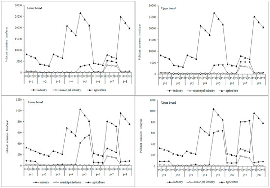
Figure 6.
Chemical oxygen demand (COD) and NH4-N emissions in the Yinma River Basin.
For the purpose of water environment protection, pollutant quantities discharged into the river should not exceed the environmental carrying capacity. Figure 7 and Figure 8 show the relationships between pollutant emission load and environmental carrying capacity for COD and NH4-N, respectively. The figures reveal that the amounts of pollutant discharged into the river decreased over time, because of reductions in regional pollutant emissions. However, the amounts were still far in excess of the environmental carrying capacities. For example, in Zone 9, the amounts of COD discharged into the river were [6638.2, 6812.7], [6196.2, 6376.0], and [5625.4, 5982.0] tons/year in three periods, which was much more than the carrying capacities of 2610.0, 2370.0, and 2130.0 tons/year. Only in Zone 10 were the pollutant amounts less than the carrying capacity. In general, there was a large imbalance between the amounts of pollutants and the environmental carrying capacities. To increase the water environment safety of the Yinma River, improvements to the water environment carrying capacity should be carried out in addition to pollutant emission reduction.
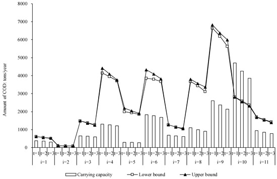
Figure 7.
Relationships between carrying capacity of COD and quantity inlets to the Yinma River.
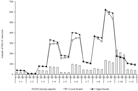
Figure 8.
Relationships between carrying capacity of NH4-N and quantity inlets to the Yinma River.
4.3. Water Environment Carrying Capacity Improvement
Table 7 lists the strategies and quantities of ecological engineering for improving the water environment carrying capacity of the Yinma River. Figure 9 and Figure 10 show the improvements in COD and NH4-N carrying capacities, respectively. These engineering projects would not be suitable for each water zone, and the quantities are constrained by the environmental conditions, resulting in different projects in different water zones. Zone 1 is the furthest upstream zone of the Yinma River and has few non-point agricultural pollutant emissions and has good water quality. Consequently, the engineering of wetlands and conservation forests would be selected, with areas of [13, 16] ha and [60, 70] ha, and capacity improvements of 310 and [42.5, 43.5] tons/year for COD and NH4-N, respectively. In Zone 3, pre-tank construction should be carried out to meet the water quality target of the lower reservoir, and dredging engineering should be carried out to improve the contaminated water quality of the river, with volumes of [0, 25] × 104 m3. Zone 6 is the main pollutant receiving water body of Region 5 and has a severely contaminated status. To address the pollution in Zone 6, [140, 150] ha of wetlands, [0, 85] km of ecological corridor, two pre-tank constructions, and [70, 80] × 104 m3 of dredging engineering would need to be implemented. This would result in improvements of COD and NH4-N carrying capacity of [1986.8, 2246.0] and [321.8, 357.4] tons/year, respectively. In Zone 10, no engineering would be needed because there is adequate environmental carrying capacity for pollutant emission loads. Artificial aeration has been proven to be an engineering solution for remediating heavily-polluted urban rivers. Consequently, in Zone 9, [700, 800] × 104 tons of artificial aeration should be carried out along with the establishment of [50, 60] ha of conservation forest and the implementation of [40, 50] × 104 m3 of dredging engineering. This would improve COD and NH4-N carrying capacity to [4030, 4325] and [1627, 1762] tons/year, respectively.

Table 7.
Projects for improving the water environment carrying capacity in the Yinma River.
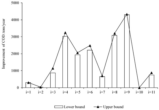
Figure 9.
Improvements in COD carrying capacity for the Yinma River.
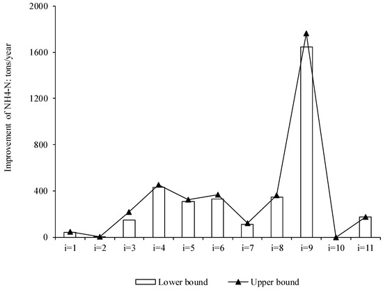
Figure 10.
Improvements in NH4-N carrying capacity for the Yinma River.
These projects that aim to improve water environment carrying capacity would not only reduce the pollutant overload, but also improve and restore the ecological environment in the Yinma River. Figure 11 and Figure 12 show that, after the implementation of the projects, there would be surplus carrying capacities under different pollutant emissions scenarios. Surplus carrying capacity is a good indicator of water ecological environment quality improvement. For example, in the Region 11 instance, the surplus carrying capacities for COD would be [3.2, 141.4], [67.7, 190.3], and [136.4, 243.4] tons/year in the three periods, and the values for NH4-N would be [114.9, 115.0], [116.5, 117.6], and [117.9, 119.8] tons/year, respectively.
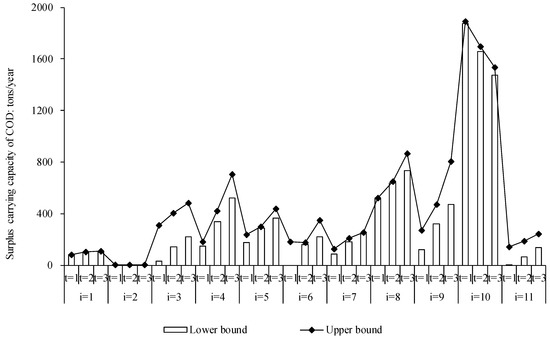
Figure 11.
Surplus COD carrying capacity for the Yinma River.
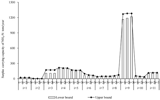
Figure 12.
Surplus NH4-N carrying capacity for the Yinma River.
5. Conclusions
In this study, an ITSP model was developed for the management of water resources and environmental carrying capacity under uncertainties. The model was applied to the Yinma River Basin, where water shortages and high degrees of contamination are found that are typical for China. The proposed model can simultaneously deal with uncertainties presented as interval values and probability distributions by integrating the IPP and TSP methods. By solving the ITSP model, the optimal water resources allocations for the four main water use sectors were determined for the planning periods under different scenarios. In addition, the amounts of pollutant emission from the different sectors in the administrative regions were obtained. These results, constrained by regional total amount control, can provide a basis for regional emission permit systems for the different sectors. Furthermore, water environment improvement schemes should be formulated for each sector to remediate the effects of contamination, and to reconcile the total regional amounts of pollution and environmental carrying capacities. The results would be valuable for guiding the optimal allocation of water resources and water quality management in the Yinma River Basin.
The aim of this study was to use the ITSP model to create a water management system that combined water resources allocation with water environment treatment strategies. This system considered water environment improvement projects together with water resources allocation and total pollutant limits for the first time. The results suggest that this approach is applicable and effective for the management of water resources allocation and water quality in the Yinma River Basin, and that the approach could also be applied in other water-stressed or contaminated areas. However, there is still much room for improvement in the proposed model. This model does not consider the decision risk under uncertainty. In addition, details such as different water sources, climate change influence on the water resources availability, the water use pattern in different sectors, and efficiencies of different wastewater treatment methods were not modeled in this study. Further studies are needed to address these limitations.
Author Contributions
Chong Meng designed the manuscript, developed the models, and wrote the manuscript; Xiaolei Wang collected the data and revised the manuscript; Yu Li checked the content and revised the manuscript. All authors made contributions to the study and the writing of the manuscript.
Funding
This research was funded by the Finance Department of Jilin Province, China (2013-931).
Conflicts of Interest
The authors declare no conflict of interest.
References
- Ran, L.; Lu, X.X. Redressing China’s strategy of water resource exploitation. Environ. Manag. 2013, 51, 503–510. [Google Scholar] [CrossRef] [PubMed]
- Xia, J.; Qiu, B.; Li, Y.Y. Water resources vulnerability and adaptive management in the Huang, Huai and Hai river basins of China. Water Int. 2012, 37, 523–536. [Google Scholar] [CrossRef]
- Gao, Q.Z.; Zhang, X.; Brendan, P.M. Study on water resources management in economic development in the water-shortage regions-a case study in the Shiyang River Basin. Arid Zone Res. 2008, 275, 2372–2384. [Google Scholar]
- Miloradov, M.V.; Mihajlović, I.; Vyviurska, O.; Cacho, F.; Radonić, J.; Milić, N.; Ivan Spanik, I. Impact of wastewater discharges to Danube surface water pollution by emerging and priority pollutants in the vicinity of Novi sad, Serbia. Fresenius Environ. Bull. 2014, 23, 2137–2145. [Google Scholar]
- Sun, J.; Chen, Y.; Zhang, Z.; Wang, P.; Song, X.; Wei, X.; Feng, B. The spatio-temporal variations of surface water quality in China during the “Eleventh Five-Year Plan”. Environ. Monit. Assess. 2015, 187, 1–12. [Google Scholar] [CrossRef] [PubMed]
- Rode, M.; Suhr, U. Uncertainties in selected river water quality data. Hydrol. Earth Syst. Sci. 2007, 11, 863–874. [Google Scholar] [CrossRef]
- Zhang, Y.M.; Huang, G.H. Optimal water resource planning under fixed budget by interval-parameter credibility constrained programming. Eng. Optim. 2011, 43, 879–889. [Google Scholar] [CrossRef]
- Nikoo, M.R.; Kerachian, R.; Poorsepahy-Samian, H. An Interval Parameter Model for Cooperative Inter-Basin Water Resources Allocation Considering the Water Quality Issues. Water Resour. Manag. 2012, 26, 3329–3343. [Google Scholar] [CrossRef]
- Jin, L.; Huang, G.; Fan, Y.; Nie, X.; Cheng, G. A Hybrid Dynamic Dual Interval Programming for Irrigation Water Allocation under Uncertainty. Water Resour. Manag. 2012, 26, 1183–1200. [Google Scholar] [CrossRef]
- Liu, Y.; Cai, Y.P.; Huang, G.H.; Dong, C. Interval-parameter chance-constrained fuzzy multi-objective programming for water pollution control with sustainable wetland management. Procedia Environ. Sci. 2012, 13, 2316–2335. [Google Scholar] [CrossRef]
- Fu, Q.; Zhao, K.; Liu, D.; Jiang, Q.; Li, T.; Zhu, C. The Application of a Water Rights Trading Model Based on two-Stage Interval-Parameter Stochastic Programming. Water Resour. Manag. 2016, 30, 2227–2243. [Google Scholar] [CrossRef]
- Liu, M.; Nie, G.; Hu, M.; Liao, R.; Shen, Y. An Interval-parameter Fuzzy Robust Nonlinear Programming Model for Water Quality Management. J. Water Resour. Prot. 2013, 5, 12–16. [Google Scholar] [CrossRef]
- Mo, S.; Duan, H.; Shen, B.; Wang, D. Interval Two-Stage Stochastic Integer Programming for Urban Water Resource Management under Uncertainty. J. Coastal Res. 2015, 73, 160–165. [Google Scholar] [CrossRef]
- Cardwell, H.; Ellis, H. Stochastic dynamic programming models for water quality management. Water Resour. Res. 2010, 29, 803–813. [Google Scholar] [CrossRef]
- Huang, G.H.; Loucks, D.P. An Inexact Two-stage stochastic Programming Model for Water Resources Management under Uncertainty. Civ. Eng. Syst. 2000, 17, 95–118. [Google Scholar]
- Maqsood, I.; Huang, G.H.; Yeomans, J.S. An interval-parameter fuzzy two-stage stochastic program for water resources management under uncertainty. Eur. J. Oper. Res. 2005, 167, 208–225. [Google Scholar] [CrossRef]
- Xu, Y.; Huang, G.H.; Qin, X.S. Inexact two-stage stochastic robust optimization model for water resources management under uncertainty. Environ. Eng. Sci. 2009, 26, 1765–1776. [Google Scholar] [CrossRef]
- Xie, Y.L.; Huang, G.H.; Li, W.; Li, J.B.; Li, Y.F. An inexact two-stage stochastic programming model for water resources management in Nansihu Lake Basin, China. J. Environ. Manag. 2013, 127, 188–205. [Google Scholar] [CrossRef] [PubMed]
- Li, W.; Wang, B.; Xie, Y.L.; Huang, G.H.; Liu, L. An inexact mixed risk-aversion two-stage stochastic programming model for water resources management under uncertainty. Environ. Sci. Pollut. Res. 2015, 22, 2964–7295. [Google Scholar] [CrossRef] [PubMed]
- Zhang, L.; Li, C.Y. An Inexact Two-Stage Water Resources Allocation Model for Sustainable Development and Management Under Uncertainty. Water Resour. Manag. 2014, 28, 3161–3178. [Google Scholar] [CrossRef]
- Ji, L.; Sun, P.; Ma, Q.; Jiang, N.; Huang, G.H.; Xie, Y.L. Inexact Two-Stage Stochastic Programming for Water Resources Allocation under Considering Demand Uncertainties and Response-A Case Study of Tianjin, China. Water 2017, 9, 414. [Google Scholar] [CrossRef]
- Xie, Y.L.; Huang, G.H. Development of an inexact two-stage stochastic model with downside risk control for water quality management and decision analysis under uncertainty. Stochastic Environ. Res. Risk. Assess. 2014, 28, 1555–1575. [Google Scholar] [CrossRef]
- Yin, H. Study on Environmental Carrying Capacity and Total Amount Control in Main Rivers of Changchun City; Jilin University: Changchun, China, 2004. [Google Scholar]
- Zhang, W.J.; Wang, Q.; Wu, Y.Y.; Ye, W.L.; Wen, Y.L.; Liu, Y.L. Characteristics of total water pollutant control in China. Environ. Pollut. Control 2016, 38, 104–109. [Google Scholar]
- Gregoire, C.; Elsaesser, D.; Huguenot, D.; Lange, J.; Lebeau, T.; Merli, A.; Mose, R.; Passeport, E.; Payraudeau, S.; Schuetz, T.; et al. Mitigation of agricultural nonpoint-source pesticide pollution in artificial wetland ecosystems. Environ. Chem. Lett. 2009, 7, 205–231. [Google Scholar] [CrossRef]
- Li, X.N.; Song, H.L.; Li, W.; Lu, X.W.; Nishimura, O. An integrated ecological floating-bed employing plant, freshwater clam and biofilm carrier for purification of eutrophic water. Ecol. Eng. 2010, 36, 382–390. [Google Scholar] [CrossRef]
- Zhenyu, A.N.; Zeng, G.; Zhang, S.; Min, X.U.; Wang, L. Effect of dredging engineering on water environmental capacity of Lake Dongting. J. Lake Sci. 2006, 18, 509–514. [Google Scholar] [CrossRef]
- Ouellet-Plamondon, C.; Chazarenc, F.; Comeau, Y.; Brisson, J. Artificial aeration to increase pollutant removal efficiency of constructed wetlands in cold climate. Ecol. Eng. 2006, 27, 258–264. [Google Scholar] [CrossRef]
- Kraaijenbrink, P.D.A.; Bierkens, M.F.P.; Lutz, A.F.; Immerzeel, W.W. Impact of a global temperature rise of 1.5 degrees Celsius on Asia’s glaciers. Nature 2017, 549, 257. [Google Scholar] [CrossRef] [PubMed]
- Shrestha, N.K.; Du, X.; Wang, J. Assessing climate change impacts on fresh water resources of the Athabasca River Basin, Canada. Sci. Total Environ. 2017, 601–602, 425–440. [Google Scholar] [CrossRef] [PubMed]
- Faramarzi, M.; Abbaspour, K.C.; Schulin, R.; Yang, H. Modelling blue and green water resources availability in Iran. Hydrol. Process. 2009, 23, 486–501. [Google Scholar] [CrossRef]
- Faramarzi, M.; Abbaspour, K.C.; Vaghefi, S.A.; Farzaneh, M.R.; Zehnder, A.J.; Srinivasan, R.; Yang, H. Modeling impacts of climate change on freshwater availability in Africa. J. Hydrol. 2013, 480, 85–101. [Google Scholar] [CrossRef]
- Rodríguez-Blanco, L.M.; Arias, R.; Taboada-Castro, M.M.; Nunes, J.P.; Keizer, J.J.; Taboada-Castro, M.T. Potential Impact of Climate Change on Suspended Sediment Yield in NW Spain: A Case Study on the Corbeira Catchment. Water 2016, 8, 444. [Google Scholar] [CrossRef]
- Adem, A.A.; Tilahun, S.A.; Ayana, E.K.; Worqlul, A.W.; Assefa, T.T.; Dessu, S.B.; Melesse, A.M. Climate Change Impact on Sediment Yield in the Upper Gilgel Abay Catchment, Blue Nile Basin, Ethiopia. In Landscape Dynamics, Soils and Hydrological Processes in Varied Climates; Melesse, A.M., Abtew, W., Eds.; Springer International Publishing: Cham, Switzerlands, 2016; pp. 615–644. [Google Scholar]
- Shrestha, N.K.; Wang, J. Predicting sediment yield and transport dynamics of a cold climate region watershed in changing climate. Sci. Total Environ. 2018, 625, 1030–1045. [Google Scholar] [CrossRef]
- Zhou, Y.; Xu, J.Y.; Xiao, W.; Wang, J.; Huang, Y.; Yang, H. Climate Change Impacts on Flow and Suspended Sediment Yield in Headwaters of High-Latitude Regions—A Case Study in China’s Far Northeast. Water 2017, 9, 966. [Google Scholar] [CrossRef]
- Hosseini, N.; Johnston, J.; Lindenschmidt, K.-E. Impacts of Climate Change on the Water Quality of a Regulated Prairie River. Water 2017, 9, 199. [Google Scholar] [CrossRef]
- Rostami, S.; He, J.; Hassan, K.Q. Riverine Water Quality Response to Precipitation and Its Change. Environments 2018, 5, 8. [Google Scholar] [CrossRef]
- Zabaleta, A.; Meaurio, M.; Ruiz, E.; Antigüedad, I. Simulation Climate Change Impact on Runoff and Sediment Yield in a Small Watershed in the Basque Country, Northern Spain. J. Environ. Qual. 2014, 43, 235–245. [Google Scholar] [CrossRef] [PubMed]
- Cong, Y.F. Study on Rational Allocation of Water Resources in Yinma River Based on the Regional Water Resource Carrying Capacity; Jilin University: Changchun, China, 2010. [Google Scholar]
- Shi, F.Z. Research on Groundwater Sustainable Yield in Medium and Small Basins of North China-Case Study of Yinma River Basin; Jilin University: Changchun, China, 2009. [Google Scholar]
© 2018 by the authors. Licensee MDPI, Basel, Switzerland. This article is an open access article distributed under the terms and conditions of the Creative Commons Attribution (CC BY) license (http://creativecommons.org/licenses/by/4.0/).