End Use Level Water and Energy Interactions: A Large Non-Residential Building Case Study


1
College of Engineering and Informatics, National University of Ireland, Galway H91 TK33, Ireland
2
Ryan Institute, National University of Ireland, Galway H91 TK33, Ireland
3
Informatics Research Unit for Sustainable Engineering, National University of Ireland, Galway H91 TK33, Ireland
*
Author to whom correspondence should be addressed.
Water 2018, 10(6), 810; https://doi.org/10.3390/w10060810
Submission received: 11 May 2018
/
Revised: 13 June 2018
/
Accepted: 15 June 2018
/
Published: 19 June 2018
(This article belongs to the Special Issue Carbon Footprint of Water Supply and Wastewater Treatment)
Abstract
:Within the European Union, buildings account for around 40% of the energy use and 36% of CO2 emissions, thus representing a significant challenge in the context of recent EU directives that require all new buildings to be nearly zero-energy by 2020. Reduced consumption of water, and hot water in particular, provides a significant opportunity to reduce energy consumption. While there have been numerous studies pertaining to the water-energy nexus of residential buildings, the complexity of water networks in larger buildings has meant that this area has been relatively unexplored. The paper presents a comprehensive investigation of the hot water use profile, associated energy use, on-site pumping energy use, carbon emissions, and solar energy harvesting potential in an Irish university building over periods before and after water conservation efforts. Total water-related energy consumption (including the heating and pumping losses) were analysed using the WHAM model and modified pumping energy expressions. The results revealed that water heating including losses contributed to as high as 30% of total building energy consumption, and stringent water conservation measures reduced the average hot water use rate by 8.5 m3/day. It was found that 10% of the total pumping energy was constituted by pump start-ups. Simulation results for solar harvesting potential in the study site found that around 60% of water heating energy demand could be met by solar energy in the new water demand scenario. The study results can act as a benchmark for similar buildings, and the model combination can be emulated in future studies.
1. Introduction
The energy and water performances of buildings are two main legislations of European Union (EU). According to the European Commission [1], buildings constitute around 40% of the energy use and 36% of CO2 emissions in EU; its directive on energy performance of buildings requires all new buildings to be nearly zero-energy buildings (nZEB) by 2020. In Ireland, standards for such buildings fall under building regulations and are referred to as near zero energy building standards [2]. In Ireland, all new buildings will have to achieve a 60% improvement in energy performance by 2020 from current levels, and 20% of the primary energy use must be supplied by renewable energy sources [3]. For all existing buildings in Ireland, major renovations (more than 25% of the total floor area) must be carried out to achieve the nZEB targets [3]. Space heating and heating water constitute 79% of total energy use in EU households [4]. A methodology aimed at demand side energy efficiency activities is being developed by the United Nations Framework Convention on Climate Change (UNFCCC) to install water saving devices in buildings from a Clean Development Mechanism (CDM) perspective [5]. Similar legislation and guidelines are being implemented worldwide to tackle the issue of increased interdependence between water and energy, which is commonly called the water-energy nexus. Recently, there has been increased attention on the energy intensity of the water sector both in terms of water and wastewater supply, disposal, and treatment, and in terms of water consumption in residential and non-residential buildings [6].
While significant attention has focused on energy intensive areas such as inter-basin transfers and desalination, energy consumption associated with water end use is less studied [7]. Water-related energy intensity associated with the end use stage in an urban water cycle has been reported at 79% of total water-related energy use in Australia, 72% in California, U.S, and 96% in Ontario, Canada; in all cases, more than 90% of this is for water heating [8]. Domestic hot water (DHW) is responsible for around 22% of household energy use in the UK [9]. According to the UK Environmental Agency [10], about 89% of total carbon emissions from water-related operations were contributed by residential water end use. Energy use associated with water consumption is far more significant than that for the delivery of water and wastewater services [11,12,13,14]. The energy requirement for domestic hot water is 16% of the total household energy requirement in the European Union (EU) [15], while it is 23% in Australia [16]. However, analysing water-related energy consumption can be complex, given the fact that end use is heterogeneous in nature, and scenarios range from a single household with single occupancy to large commercial and industrial estates and various public buildings.
State of the Art
There have been a number of studies that describe various aspects of end use water consumption and related energy uses; almost all of them were conducted on a household/residential level (Table 1).
Hendron and Burch [31] found that the drivers of DHW events were occupant behaviour (event timing, duration and frequency), occupant number, household income, climate and season, and efficiency of water-related appliances, of which occupant behaviour was the most important. Similarly Merrigan [32] found that occupant rate has a linear relationship with DHW use. Local climate and seasonal variation played an important role in residential DHW, as found in a study by Goldner [33], in which DHW consumption volume was found to increase by 13% from summer to winter in New York. The seasonal variation of water consumption (30–48% seasonal differences) was noted to be more significant in Australia [34]. But these studies did not investigate associated energy use.
Bohm [35] noted that energy meters were rarely used to measure the energy use of hot water systems separately in buildings, and thus, this aspect is not separated from energy used for space heating. Bohm, Danig [36] and Schroder [37] documented that DHW contributed not only high energy in apartment buildings, but also incurred high distribution losses. Similar studies [38,39,40,41] pertaining to hot water use and associated energy consumption in buildings, also on small residential buildings, have been undertaken. Almost all studies regarding water associated energy use have not focused on non-residential buildings [42]. This may be due to the fact that water demand for residential end uses is mainly contributed by showers, clothes washers, toilets, dishwashers and baths [43], but the demand in non-residential buildings can have these and many other end-uses. A comparison of hot water consumption profiles in different non-residential building types by Fuentes et al. [42] indicated that there existed significant differences among them, which warranted a detailed building water use profile characterization. They [42] also found that information on hot water use profiles for non-residential buildings were limited, and hence required additional studies based in different geographical zones and climates.
In Ireland, buildings were the second largest consumers of energy end use after the transport sector [44]. In 2014, buildings consumed 35% of total energy and 59% of all electricity in Ireland. Though around 90% of total energy in Ireland is imported, and hence its efficient management is paramount, energy use of the water sector has received limited attention in Ireland. The ratio of water extraction to water availability is low (2%) in Ireland compared to the higher ratios in some other European countries such as Belgium and Spain [45]. Perhaps as a result of this, the hidden economic and energy costs involved in treatment, end use, and disposal of water are often overlooked [45].
This study focused on the energy consumption associated with water end use in a large non-residential building with the following key objectives:
- Characterisation of hot water use and total water use in a large case-study building before and after implementation of water conservation measures
- Characterisation of energy use and CO2 emissions associated with water heating and pumping
- Estimation of energy losses associated with water heating and pumping using comprehensive models
- Benchmarking of energy and CO2 emissions
- Potential of a solar energy harvesting system as an energy source for water heating
The main contributions of the proposed study are therefore to increase the understanding of average energy consumption and associated CO2 emission intensities of water-related activities across various time scales in a large non-residential building in a west European context. This study will further help in benchmarking water-related energy use (both pumping and heating), which is required for the design of renewable energy integration and demand side management strategies.
2. Materials and Methods
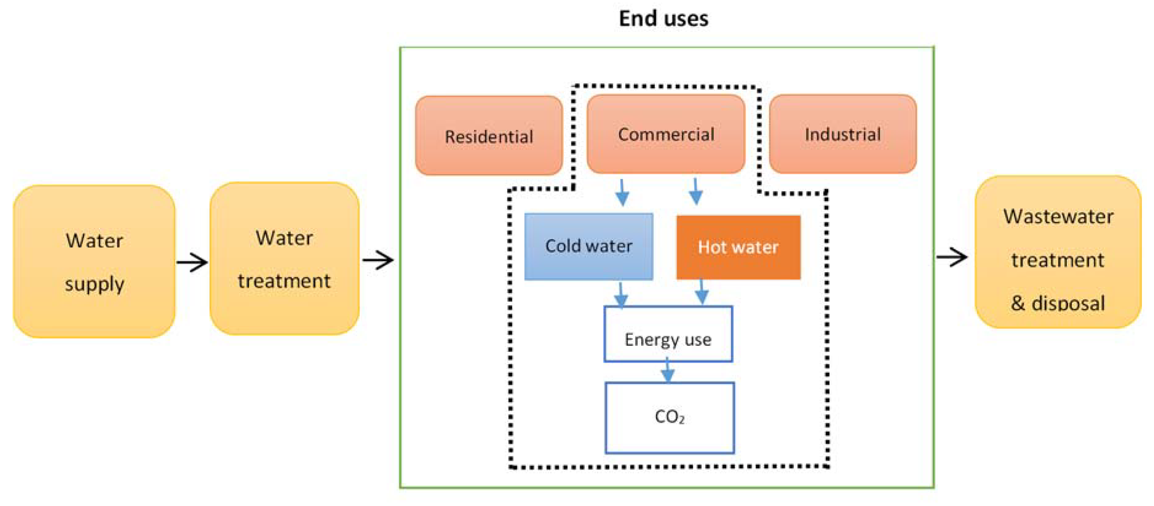
The water-energy relationship begins with water supply from the source, followed by its treatment, end uses, wastewater treatment, and finally, disposal. There are three main types of water customers in an urban context: residential, commercial, and industrial. This study focused on the energy expended and associated CO2 emissions for water-related activities on a building scale, as outlined by the system boundary (dashed line) in Figure 1. Water-related energy use comprised heating and pumping in the building; the other energy uses in the building were mainly space heating, lighting, electronics, lab equipment, and miscellaneous uses.
The description of the building (case study site) and data collection are given in Section 2.1 and Section 2.2.
2.1. Case Study
The engineering building at National University of Ireland, Galway (NUIG) was chosen as the site for the present case study as it was designed as a smart building and has water and energy meters installed at various locations. The state of the art engineering building at NUIG houses about 1100 students and about 100 staff during teaching and exam terms (approximately 26–28 weeks in total), and about 100 staff and 100 postgraduates during the rest of the year. The building includes lecture halls, classrooms, offices, laboratory facilities, a cafe, and shower and toilet facilities spread across 14,000 m2 of floor space on four storeys. Thus, it has a variety of end-uses for water, and significant variation in how water is used. The building is managed through a Building Management System (BMS) that collects data on building performance and operational efficiency—including 11 water meters. Some of the key water users include showers and hand wash basins, grey water from a rainwater harvesting system for toilets and urinals, and potable water for the water fountains and café. As this study was dealing with only water heating and pumping, their detailed descriptions are given in the following sections. Further details of the case study building water network are available at Clifford et al. [46].
2.1.1. Building Pumping System
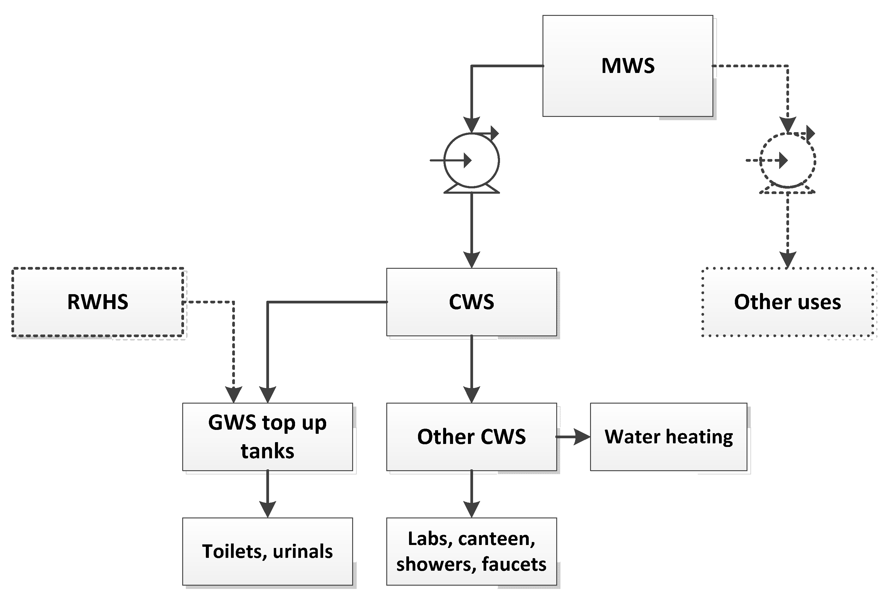
The mains water system (MWS) in the building is divided into a cold water system (CWS) and potable water supply for drinking fountains, a café and other similar uses. There are two sets of booster pumps (Figure 2), each for pumping the CWS water and other water supply. The other uses are negligible (6% of the total use, and mostly supplied for drinking water fountains) compared to the total CWS water use in the site, and hence, are ignored for pumping calculations. The total CWS water is then divided into water for grey water systems (GWS) and other uses like labs, hot water mixing in showers and faucets, and the canteen. The grey water system supplies water to the building’s toilets and urinals. The building has a large rainwater harvesting system (RWHS) for supplying grey water. When the RWHS cannot supply sufficient grey water, two CWS tanks located on roof tops (8 m3 capacity each) are used to top up the GWS. During the study period, the building RWHS were not working due to some system faults. Hence, the pumping load calculation in this study included booster pumping for GWS and other uses.
2.1.2. Building Hot Water System (HWS)
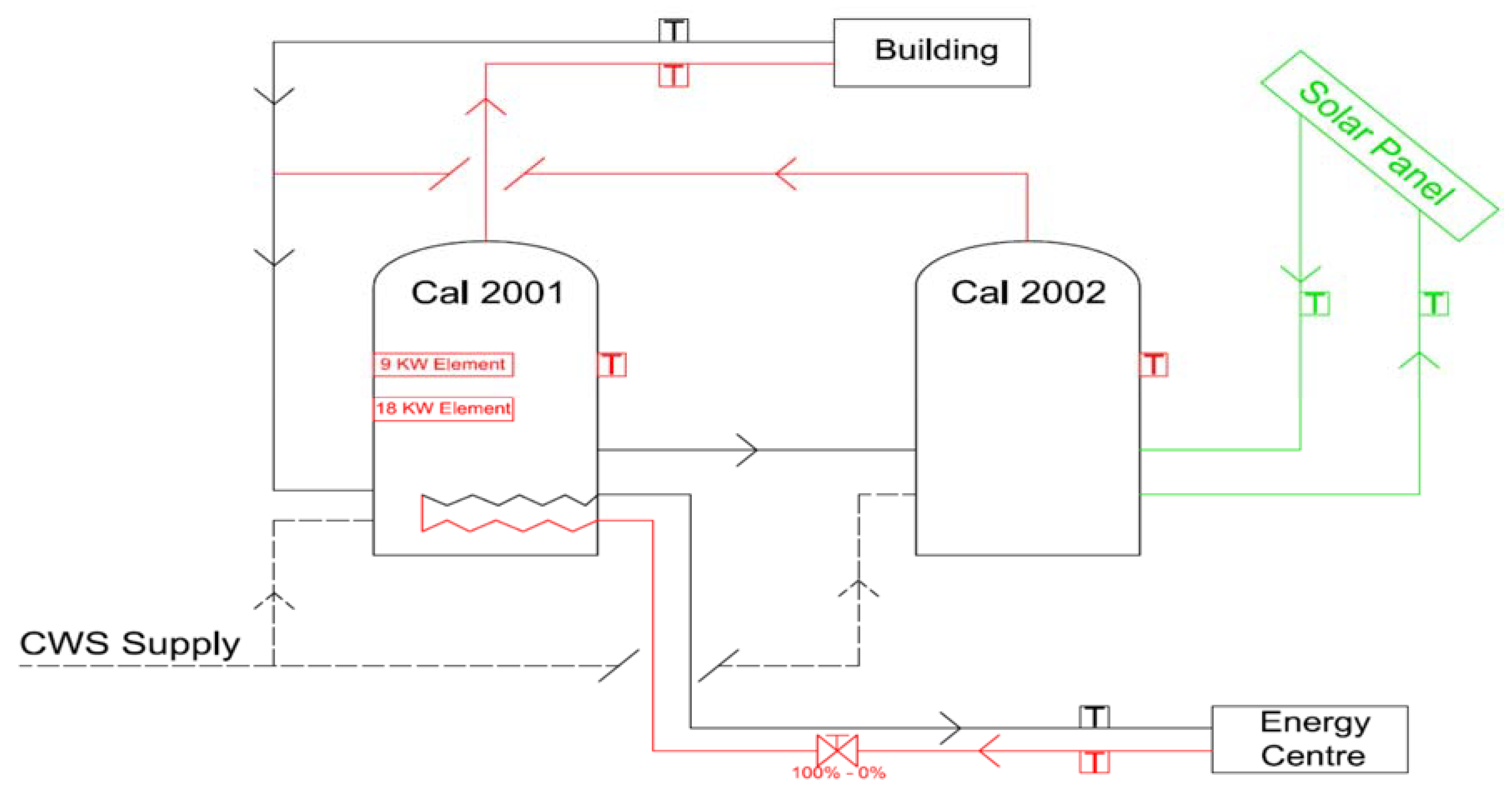
In the study site building, the water was heated to a required temperature (usually 60 °C) using a centralized natural gas heating system located in an adjacent building, and circulated through a calorifier system on the second floor of the building, as shown in Figure 3. One calorifier (Cal 2001) is used to transfer the heat from the source to the cold water coming from the cold water system (CWS). The hot water system was designed such that the water would be pre-heated in a second calorifier (Cal 2002) using solar energy before being transferred to Cal 2001. However, the system has not been commissioned. The cold water feed is brought into the solar cylinder to heat the coldest water, in order to maximise the use of renewable energy. As per the operations manual, the solar energy potential of the system installed on the building roof is supposed to yield 20 kWh/day from an area of 12 m2 solar panels. The hot water produced is then circulated to various end uses such as showers and faucets. The current study did not disaggregate hot water end users.
2.1.3. Data Measurement and Collection
A building management system (BMS) collected hot water and cold water use data separately. Hot water use data was metered using an ultrasonic flowmeter (Micronics USF1000™, Buckinghamshire, UK). The meter was set such that one pulse represents one litre of hot water used, and the number of pulses per minute was logged. The readings were aggregated to get hourly and daily values. For this study, the data prior to and post implementation of water conservation measures was considered (2016 and 2018). During the study and as part of adopting sustainability measures in the building, the shower controls were changed from manual flow control to non-concussive push taps. Card access was also introduced to the male showers during the latter half of 2017. In 2016, daily data from March to December was available and used in the study, while in 2018, hourly and daily data from January to March were used. The data for 2017 was unavailable due to maintenance issues in the building. One academic year is divided into three main periods namely—Semester 1 (January to May), Semester 2 (September to December) and summer (June to August). Key non-teaching periods occur each year over summer break, Christmas, one week in Semester 1, and one week in Semester 2. During these periods staff and postgraduate students are typically working, however undergraduate students are not present. For measuring the total pumped CWS water, an in-line water meter (B Meters, Italy) was used, which was linked to the BMS. A number of end-users were also metered during the building construction, including one male and one female toilet located on the ground floor, which included sinks with hot water usage. The average daily demand for all male and female toilets was calculated by considering the total number of toilets within the building (19 male and 42 female toilets and 16 urinals), based on the assumption that toilets on ground floor had high usage of water per day. Based on a previous survey of daily occupancy rates of various toilets in the building, the water usage for different toilets on all four floors of the building were assigned as fractions of ground floor toilets. It should be noted that the building initially used intensive urinal flushing: a rate of approximately 2 L per flush with a frequency of 25 times per hour. However, as a result of water conservation measures, a more conservative flushing regime for urinals was deployed.
2.2. Energy Consumption
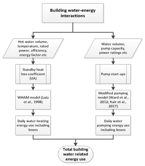
The overall methodology adopted for the estimation of energy associated with water end use is outlined in Figure 4. Water heating and pumping constituted the energy consumption associated with building water end use. The water heating energy calculation approach is explained in Section 2.2.1, while the same for pumping energy is described in Section 2.2.2.
2.2.1. Energy Consumption for Water Heating
The HWS in this case study comprised a storage water heater which heated water using natural gas. In the storage water heater, as water temperature was constantly maintained, distribution and standby heat losses were incurred. At a residential level, the energy used to maintain a steady water temperature might be insignificant, and hence, is ignored in many studies. Given the building in this case study had a relatively high level of occupancy (particularly at certain times of the year), standby heat losses were included, and the total energy expended was modelled using the Water Heater Analysis Model (WHAM) by Lutz et al. [47]:
where E = total energy used for water heating per day (kWh/day); V = daily volume of water heated in the building (m3); = density of water (1000 kg/m3); = specific heat of water (4.187 kJ/kg °C); = set temperature (°C); = inlet temperature (°C); = water heater recovery efficiency; = standby heat loss coefficient; = ambient temperature (°C); = rated input power of the heater (kW).
The WHAM model accounts for a range of operating conditions and energy efficiency characteristics of water heaters, as compared to the general expression for calculating water heating energy use. Recovery efficiency (), standby heat loss coefficient (UA), and rated input power are the efficiency parameters used in the model, whereas daily hot water draw volume, water temperature at heater inlet, water heater tank temperature, and ambient air temperature around the heater are the operating parameters. Recovery efficiency () is the ratio of energy added to the water compared to the energy input to the water heater. This accounts for the losses incurred while transferring the heat from the burner to the water. In this study, efficiency was assumed to be 76% (average of efficiencies for gas heaters at various efficiency levels as given by DoE [48]). Rated input power was taken as the nominal power rating of the water heater assigned by the manufacturer in kW (96 kW in this case). The inlet water temperature was assumed to be 5 °C more than the mains water temperature [49], and the average indoor ambient temperature was 21.5 °C in the building. The set temperature of the heater output was 60 °C.
The standby heat loss coefficient () is the rate at which energy must be added to the water heater to maintain the desired temperature when water is not heating for delivery. The unit is given by kW/°C. is given by the following expression [47]:
where, is the energy factor of the heater given by the manufacturer; is the efficiency of the heater and is the heat content of the water drawn from the heater in kW. The average energy factor (EF) or energy efficiency level for gas-fired storage water heaters was taken as 0.65 [48].
In the water heating system of the current study site, the pipes distributing hot water to various parts of the building were well insulated using mineral wool (with a thermal conductivity of 0.037 W/m·K) to avoid distribution losses. So, it was not represented in the above expression.
2.2.2. Energy Consumption for Water Pumping
In the case of residential end use, there is generally no requirement for onsite pumping, as the mains water supplied from the utility has enough pressure to maintain the flow [14]. But in the case of large buildings such as this case-study with 4 floors and facilities such as laboratories, toilets, washrooms and canteens, this pressure might not be sufficient. In such cases, additional “booster pumping” is required to maintain the water pressure.
Normally, the energy consumed for pumping water is considered only for pump operation. But in large buildings, frequent pump starting can constitute significant energy use (as high as 60% more) in addition to the energy use in pump standby mode [50,51]. Therefore, this paper considered the energy associated with pumping water during steady-state pump operation, start-ups, and stand by.
The total pumping energy required including the pump start-up energy and operating energy can be given as [50]:
where, is the total energy use for pumping water (kWh), is the power withdrawn from the electricity supply (kW), is the actual power transferred to the water (kW), is the sum of power used for pump start up and operation, and is the duration of pump operation (h).
The above expression does not consider standby energy usage of the pump when water is not being pumped. Therefore, considering that aspect and modifying the above expression, can be derived as [52]:
where is the total volume of water consumed (m3), is the pump capacity (m3/h), is the percentage of total volume pumped during the start-up phase, is the number of start-ups in a day, is the percentage of energy consumed during the start-up phase, is the power consumed during stand-by (kW), is the volume pumped during pump operation.
The number of pump start-ups can be given by Equation (5):
where, is the upper threshold volume of header tank (m3), is the lower threshold volume of header tank (m3), is the number of header tanks.
The pump power withdrawn from electricity supply is given by Equation (6), as below:
where, = system efficiency.
The energy consumption for pumping operation , as given by simple standard expression, is:
The variables and parameters for the above set of equations were acquired from the pump and water distribution system (WDS) specifications of the case study site.
2.3. Solar Energy Potential for Water Heating
The case-study building is located in the west of Ireland (approximately 12:00–13:00 h annual sunshine); the potential for solar water heaters to reduce the use of gas was analysed. Simulations were run using PVsyst V6.70™ (Satigny, Switzerland) supported by daily water demand data. Six different scenarios were run based on the available roof area for solar module installation in the building. The total effective roof area (area available minus existing building services) of the building concerned was measured as 1300 m2 for the two wings (east and west) of the site, with 650 m2 for each wing. Therefore, four scenarios were run for a combination of two periods with two different effective areas (1300 and 650 m2) given as inputs, along with energy demands for obtaining the solar potential, and another two scenarios for each year without giving areas as inputs, but based only on demands. In other words, the target goal of these simulations was to see the scenarios which best match the solar energy production and demand with respect to available effective harvesting area. For the latter two scenarios, the simulation tool gave the harvesting size as output along with energy potential. The six scenarios simulated were:
- (1)
- First year monthly demand profile using an area of 1300 m2
- (2)
- First year monthly demand profile using an area of 650 m2
- (3)
- Second year monthly demand profile using an area of 1300 m2
- (4)
- Second year monthly demand profile using an area of 650 m2
- (5)
- First year monthly demand profile without effective area as input
- (6)
- Second year monthly demand profile without effective area as input
The outputs of these scenario runs are given in Section 3.5, in which scenarios 1, 2, 3, 4, and 6 correspond to Section 3.5. Scenario 5 yielded a result with an unviable module area, which was larger than the available roof area, and hence, is not discussed further. The energy demand for water heating as estimated by the WHAM model was uploaded to the tool as a daily time-series data sheet. The place called Crinkill in County Offaly, Ireland was chosen, as it was the nearest available site in the simulation tool list.
2.4. Carbon Emissions
In order to estimate CO2 emission intensities associated with water end uses at a building level, the energy use intensity was multiplied by an equivalent CO2 emission factor according to the type of energy used. In this case study, natural gas was used to heat water, while electricity from the grid was used to operate booster pumps. The emissions from electricity use vary depending on the fuel mix used for its generation at any given time. The emission factors for various forms of energy used in Ireland are given in Table 2.
The CO2 emission intensity resulting from building level energy use was calculated by:
where, CE is the CO2 emission intensity in kgCO2/m3 due to water-related energy use in buildings, EF is the emission factor in kgCO2/kWh related to the type of energy source and EC is the energy consumption per unit quantity of water heated or pumped in kWh/m3.
3. Results and Discussion
3.1. Daily Hot Water Use
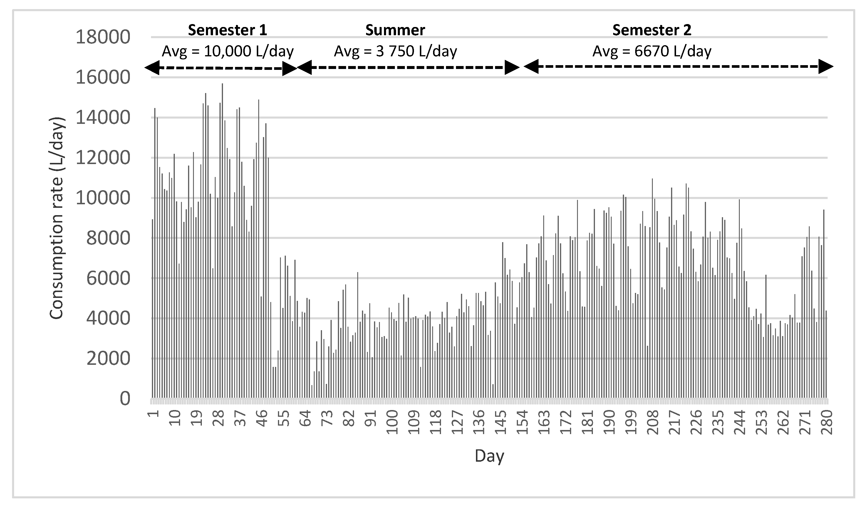
The hot water usage rate in the building over the study period is shown in Figure 5 and Figure 6. It can be seen that average water consumption during summer was around 63% lower than that of Semester 1. In the Semester 2, consumption was around 33% lower than during Semester 1. The reduction in hot water use during non-teaching periods can be attributed to the reduced occupancy rate in the building. The reduction in the average use between the first and second Semesters was probably due to an information campaign regarding shower usage in the building (as occupancy would have remained the same and no other interventions were put in place).
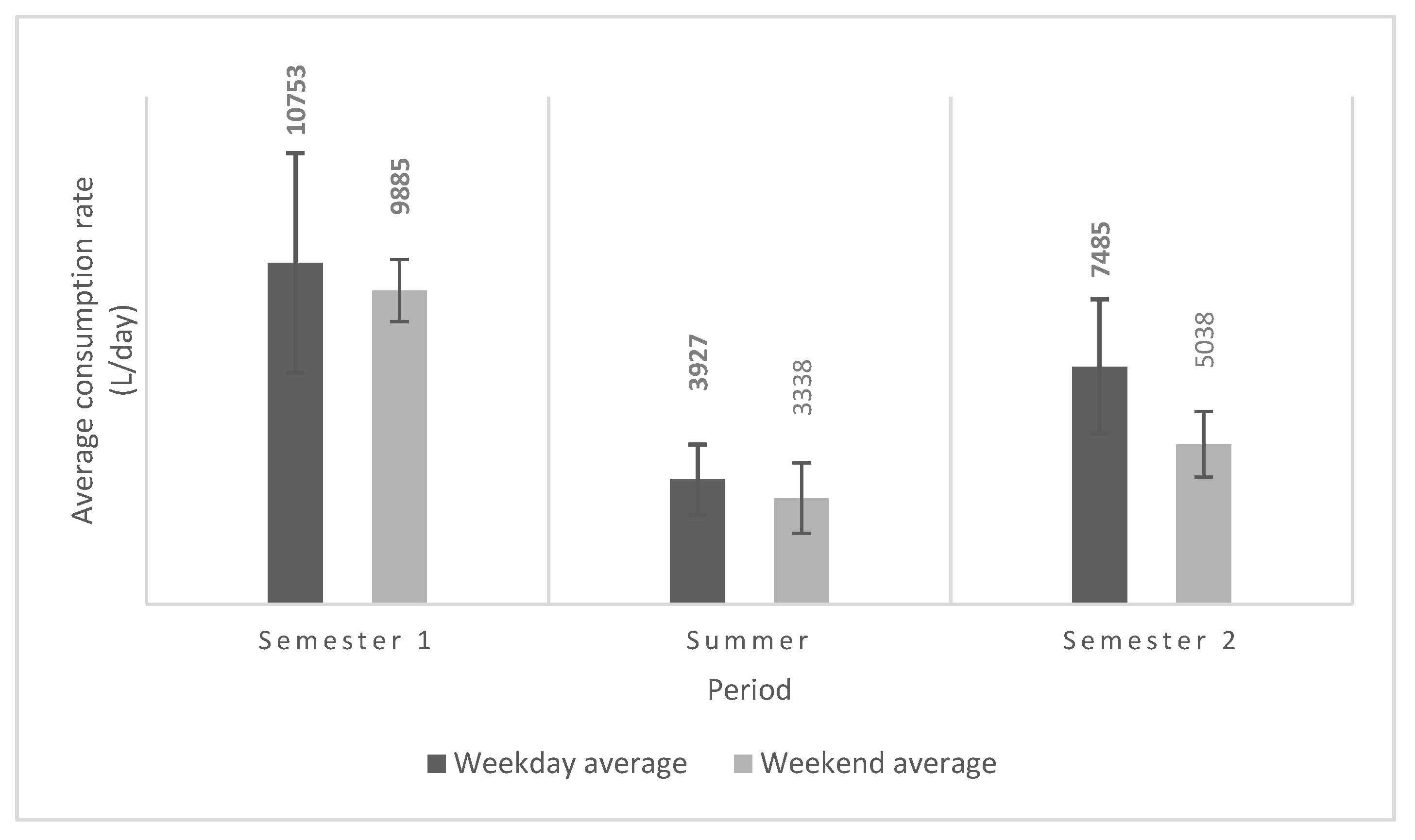
Figure 6 shows the average daily hot water use in weekdays and weekends for various semesters in 2016.
It was observed that the percentage difference between weekdays and weekends was only 8% for the first semester and 15% for the summer break. However, the percentage change increased to around 45% for the second semester, perhaps due to increased building occupancy during weekends ahead of student exams and project deadlines. The ratio of hot water use to total water use (cold water) for the building is shown in Figure 7 for weekdays, weekends, and combined use for 2016 from March to December. In the context of an academic building, the ratio would be impacted by the exact dates of the academic term. The usage ratio was generally high in the first semester and low during summer, owing to the lower occupancy rate (coinciding with non-semester). Though the ratio increased after September, when the second semester started, it is lower than that of first semester of the year. This was attributed mainly to the seasonality and an increase in inlet water temperature.
It can be seen that the ratio is relatively high (albeit decreasing) in March, April, and May; thereafter it remains relatively constant, before increasing in October. This can be due to the change in occupancy in the latter half of the year. The annual average ratio for all the profiles is similar, at 0.19. The ratios for the total use profile during first semester, summer, and second semester are 0.28, 0.13, and 0.17 respectively.
3.2. Impact of Water Conservation Measures
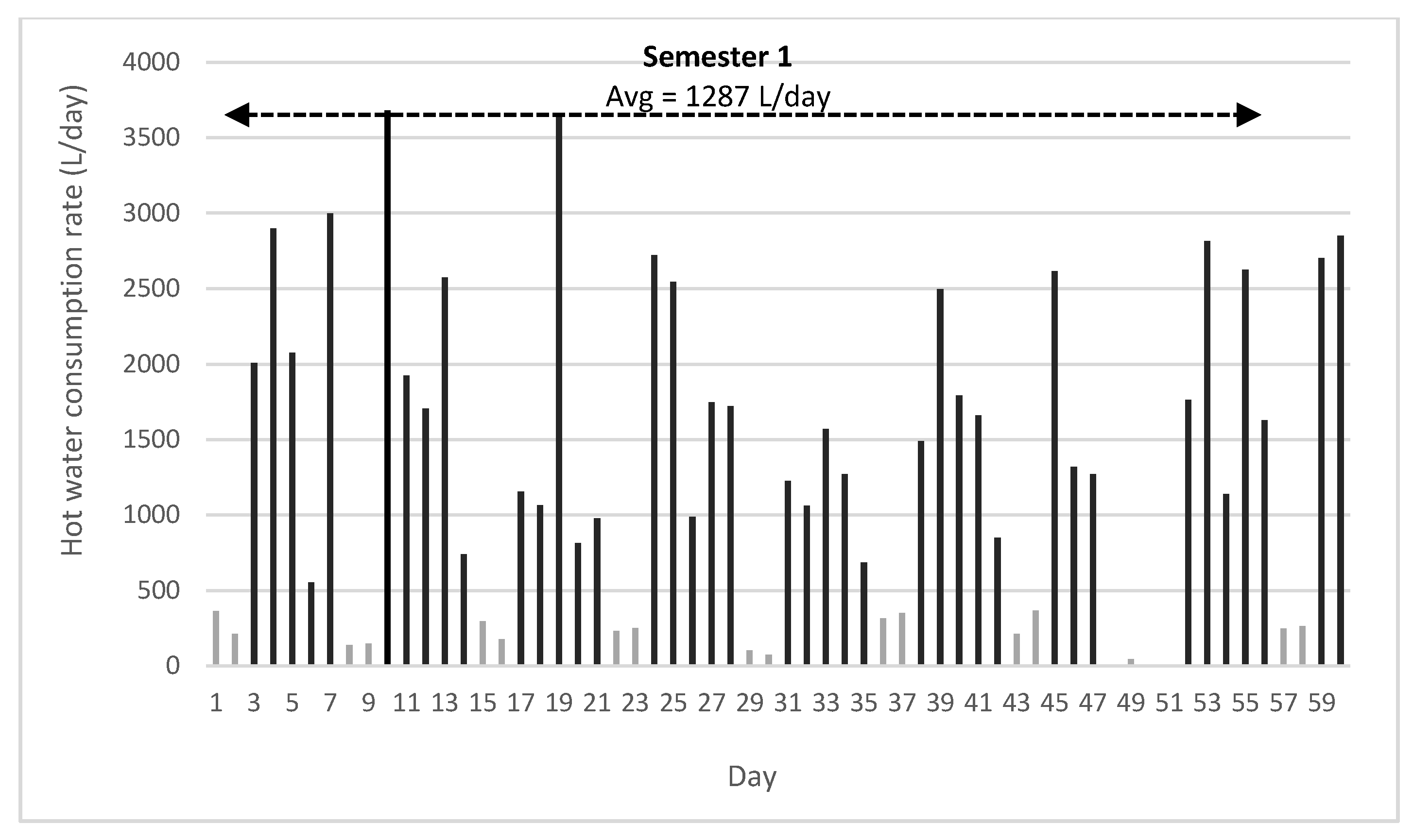
The major share of the hot water use in the building was attributed to showers. The water conservation measures, as explained in the case study section, contributed to significant reductions in hot water consumption. This is evident from Figure 8, which shows hot water use rate during the first semester of 2018. The average hot water use during this period reduced drastically to 1287 L/day, compared to that of around 10,000 L/day during the same period in 2016. The consumption rate for weekdays averaged 1749 L/day and for weekends averaged 209 L/day. The lighter lines indicate weekend days in Figure 8.
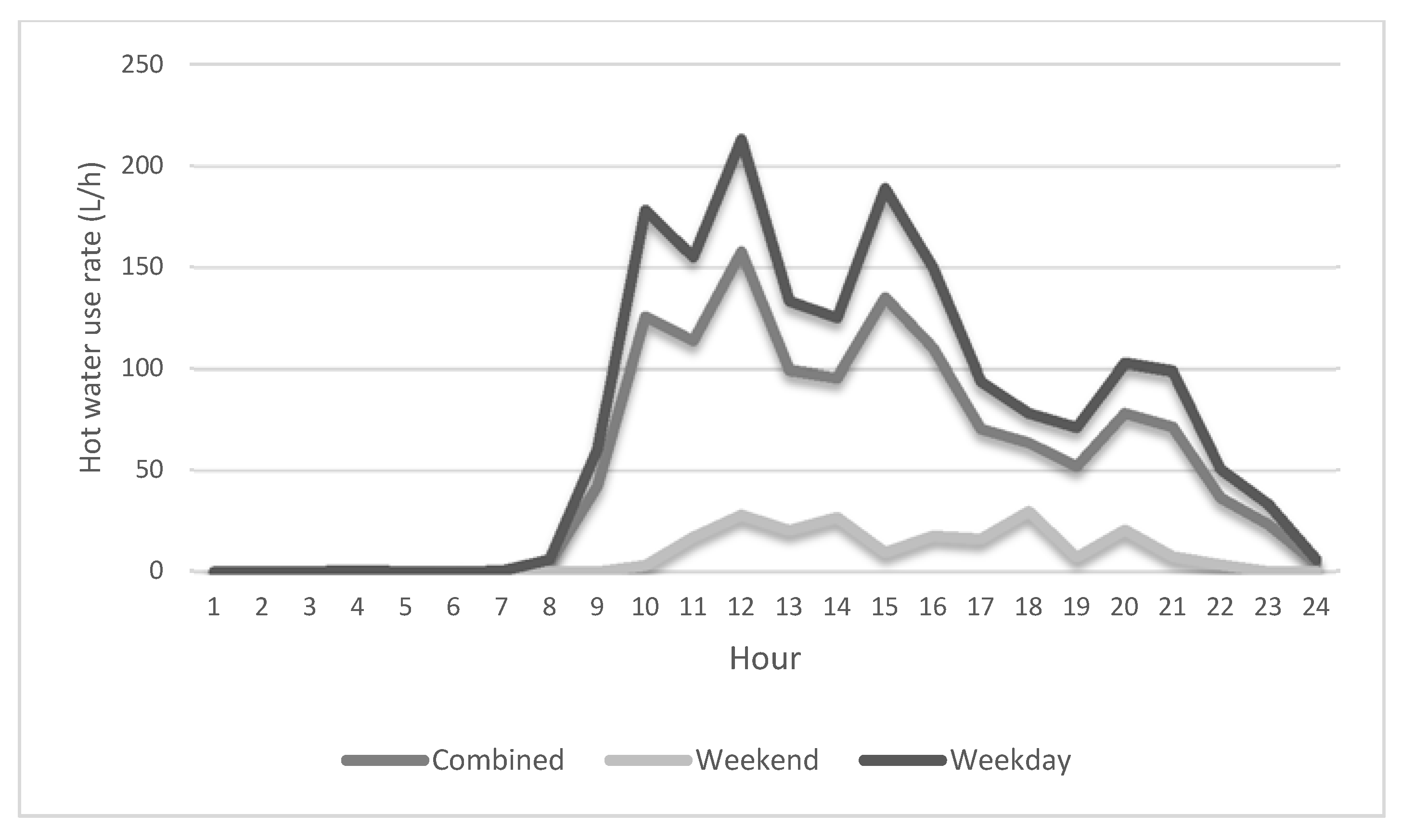
Figure 9 details the consumption of hot water on an hourly basis during first semester of 2018 after the implementation of stringent demand management measures. It should be noted that after the implementation of demand management measures, average water consumption reduced significantly. The hourly-use pattern for both weekdays and weekends shows multiple peaks during the day. This is contrary to the patterns in residential buildings, as observed by Ahmed et al. [26] in Finnish homes, Bertrand et al. [15] in homes across a number of European countries, and Fairey and Parker [53] in the US, where two peaks—one in the morning (between 7 a.m. to 10 a.m.) and another during evening (7 p.m. to 10 p.m.)—were typically observed. Furthermore, a significant difference between a weekday and weekend hourly profile, as observed in a Finnish residential building, was the rightward shift in the morning peak of weekend profile, while the water use quantity remained almost the same [26]. But for this case-study building, the major difference in the profile was the significant reduction in water consumption during the weekend, due to reduced occupancy.
While the average hourly peak during a weekday was 213 L/h around 11:00 to 12:00, the peak during a weekend day was observed to be around 30 L/h between 17:00 and 18:00.
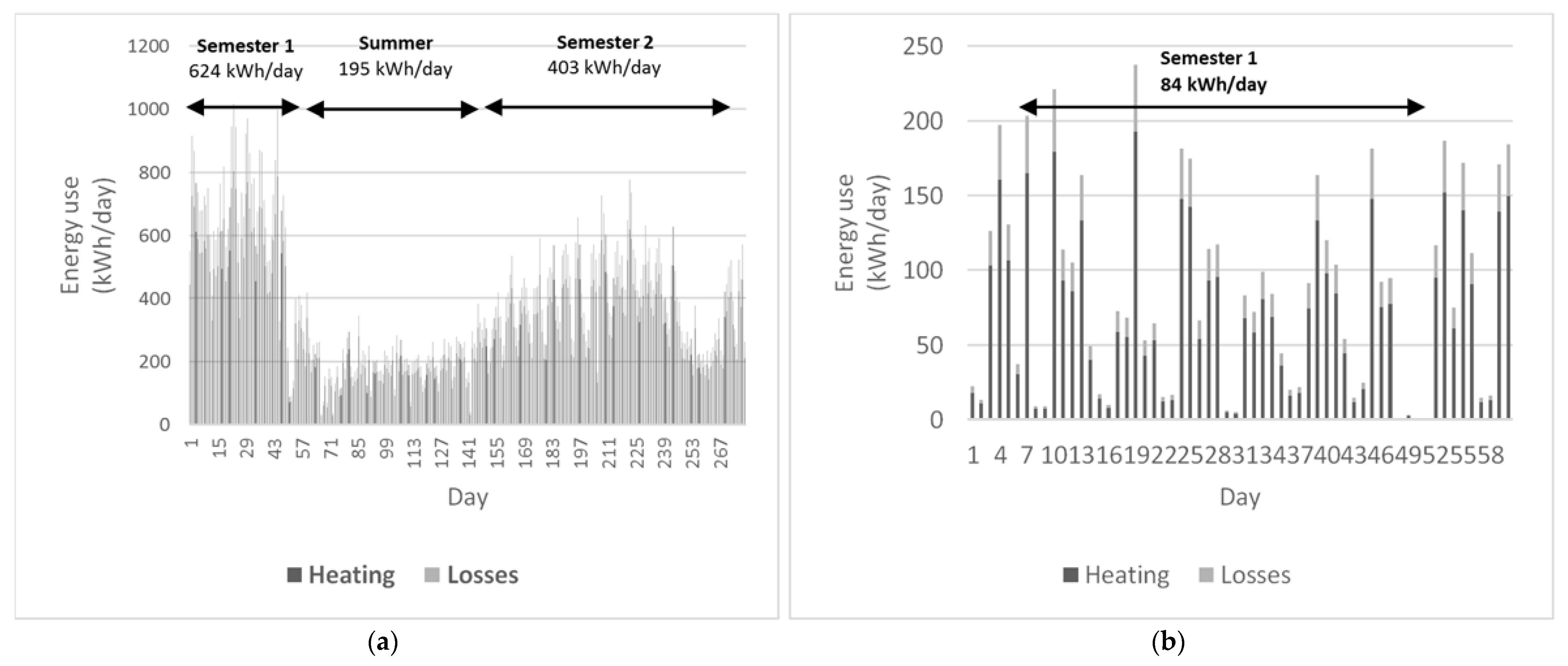
3.3. Water Heating Energy Use
The energy consumed on a daily basis for water heating in the building is shown in Figure 10. The average energy used for water heating in the first semester of 2016 was 624 kWh/day, while the same for summer and second semester were 195 kWh/day and 403 kWh/day respectively. There was a marked reduction in the energy use for Semester 1 in 2018, corresponding to the reduction in hot water use due to the implementation of water conservation measures in the building (Figure 10b). Reduced shower use during the colder period may also be due to the decreased outdoor activities of the occupants.
The average outside temperature during Semester 1 2018 was around 9 °C, with a standard deviation of 2.7 °C, while for Semester 1 2016 it was 12 °C, with a standard deviation of 1.8. Though the effect of temperature might not be significant on water use quantity, it is paramount to the impact on energy use, especially energy intensity. This was evident from the energy intensities of the different period analysed in 2016 and 2018. The water heating energy intensities of first semester, summer, and second semester in 2016 were 62, 52, and 60 kWh/m3 respectively, while it was around 65 kWh/m3 for first Semester in 2018. The variations in energy intensities across various study periods could be due to reduced heating requirements and reduced energy losses in warmer months [42]. There does not appear to be literature available regarding the energy intensities of hot water use in large buildings; thus, a direct comparison with this study is difficult. However, Fuentes et al. [42] have reported the hot water use and energy use per day for households for various countries in Europe, US, and Canada. The average European (Germany, Spain, Portugal and Switzerland) household hot water use energy intensity was around 52 kWh/m3, with the exception of UK (35 kWh/m3) and Finland (42 kWh/m3). The energy intensities of US and Canadian households were reported as 23 and 46 kWh/m3 respectively. Moreover, the energy intensities obtained in this study are high compared to other stages of the urban water cycle, as mentioned in Walsh et al. [45]. For example, the energy intensity of seawater desalination is usually considered to be the highest, falling in the range of 3–8.5 kWh/m3 [45]. Therefore, the water heating energy intensity of this building was around 7.5 times higher than that of a desalination plant. Analysis of losses associated with water heating showed that the losses for standby heating in this building were significant, at a rate of 20% of the total water heating energy use per day. The average daily energy loss was around 76 kWh during 2016, and around 16 kWh in 2018, with an average energy intensity of about 11 kWh/m3 in both years.
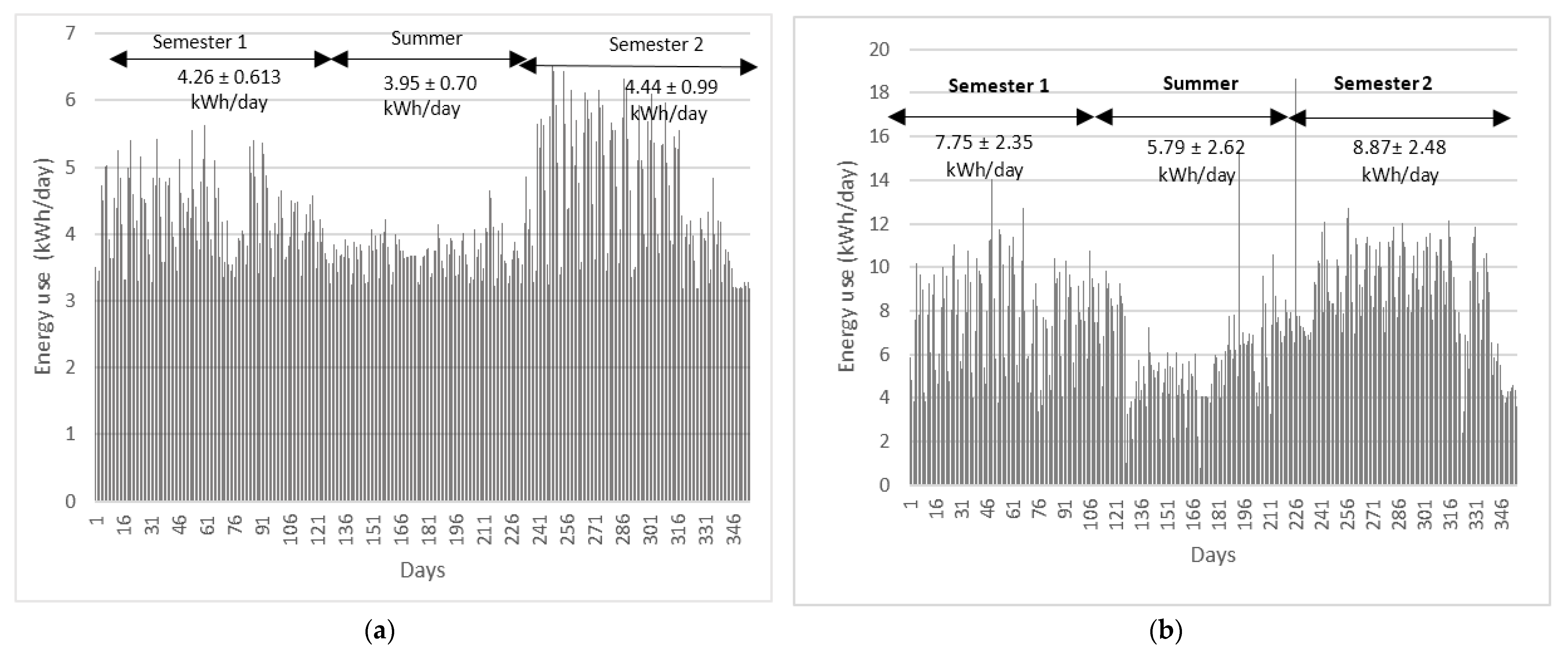
3.4. Pumping Energy
As previously discussed, the total cold water supply comprised top up water for GWS and cold water for other purposes, like hot water mixing in showers and faucets, labs, and the canteen. Figure 11a depicts the energy expended for pumping CWS to top up the GWS, while Figure 11b shows the energy used for pumping water for the remaining end uses. The average pumping energy associated with the GWS for Semester 1, summer break, and Semester 2 were 4.26, 3.95, and 4.44 kWh/day respectively, while it was 7.75, 5.79, and 8.87 kWh/day respectively for other end uses (Figure 11b). It can be seen that there was relative consistency in energy consumption for GWS pumping throughout the year, probably due to the continuous flushing of urinals (which was independent of occupancy). The average pumping energy use for both GWS and other CWS uses increased in Semester 2 due to higher CWS demand (this is contrary to the hot water trends described above). The energy intensity of the total water pumping in the building was found to be 0.34 kWh/m3, which was approximately 0.6% of the heating energy intensity observed.
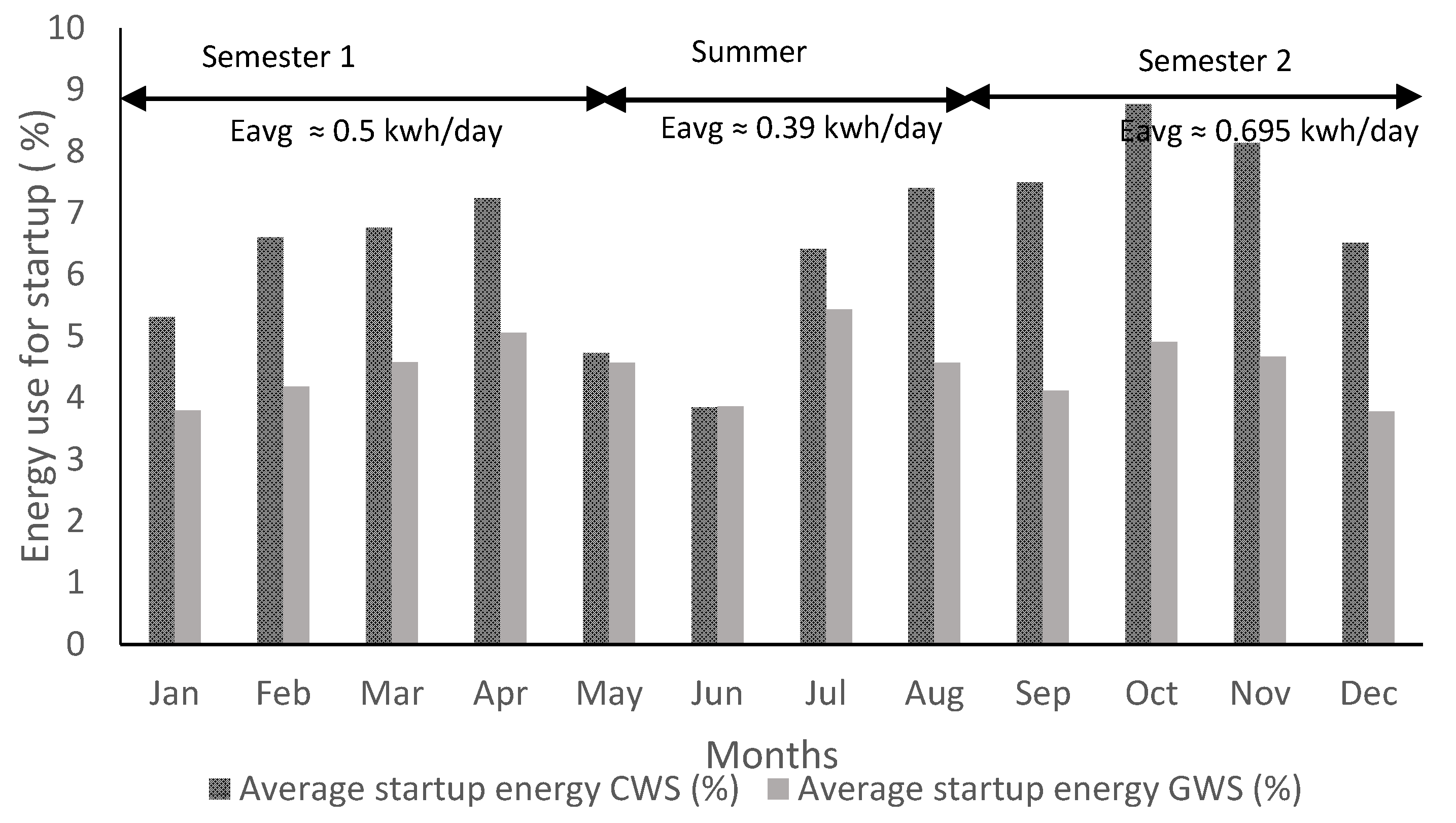
The average monthly energy consumed due to pump start-ups for GWS and other CWS uses pumping was calculated as a percentage of corresponding total pumping energy uses starting in each month of 2016 (Figure 12).
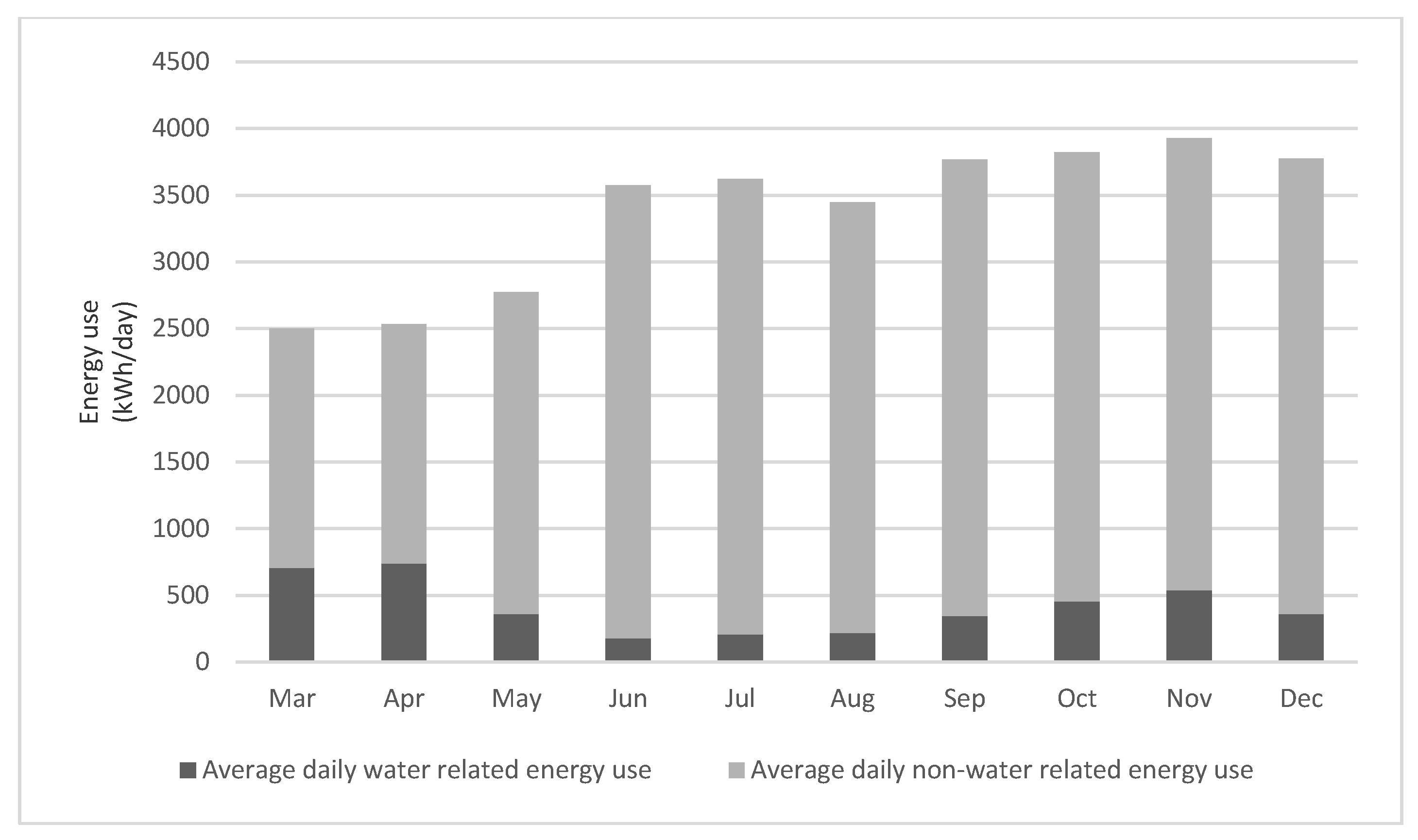
Pump start-ups contributed to around 10% of the total water pumping energy usage in the building, with 4% of that energy being consumed by the GWS, predominantly by the frequent urinal flushing. Figure 13 shows water-related energy use in the context of all energy and electricity use within the building. Water-related energy consumption was highly significant in the building for the first few months of the year, constituting around 30% of the total energy. Subsequently, the water-related energy use reduced to around 5.5% of the total energy during the summer break, and around 11% during Semester 2. It should be noted that out of the total water-related energy use in this study, heating constituted around 98%; the remainder may be attributed to pumping. These findings fall within the range of a few available literature values. Perez-Lombard [54] observed that water heating alone accounted for about 4 and 10% of the total energy use in US and UK office buildings respectively, while hot water use constituted around 30% of the total energy use in US hospitals.
The average daily water-related energy use per unit floor area for the three periods in the buildings were found to be 0.04, 0.01, and 0.03 kWh/m2. While it would be ideal to compare the present results to similar buildings with labs, teaching spaces, toilets, showers etc, the data for such building types are absent. However, comparing the energy use per unit area of this study site with that of other large building types reveals that the values lie within the same range. This is evident from the results obtained by Ulseth et al. [55] and Deng [56]. The water heating energy use per unit area for a Norway hospital was found to be 0.007 kWh/m2 [55], but 0.5 kWh/m2 [56] for a Korean hotel was. Such metrics can be used in comparing water-related energy use of other buildings in the campus and elsewhere when occupancy details are unavailable.
3.5. Solar Contribution for Water Heating
The total energy for water heating in the building calculated using the WHAM model was used as the demand profile to estimate the solar energy harvesting potential. The energy demand profiles of 2016 and 2018 were used as inputs and the contributions from the solar energy system with restrictions on available harvesting area were simulated. The solar contributions and required top up energy from the grid are shown in Figure 14.
The results showed that around 82% of total yearly heating demand in 2016 could be met using a module size of 1300 m2 (Figure 14a), with the solar energy providing full supply for the period from May to October, and around 50% for November and December 2016. Figure 14b shows that the total annual energy contribution from solar panels with a module area of 650 m2 could be around 60% of total demand. During the summer period, it could supply 100% of the heating demand, 50% for March and April, and 30% for November 2016 to January 2017. Figure 14c–e show the contributions from solar modules and grid supply for the three months of 2018 when the hot water consumption and associated energy were significantly lower than in 2016. The results showed that using a module size of 1300 m2, full heating demand could be met using solar modules, except for January 2017 (88% demand could be met), when only partial data was available. The same results were obtained when a module of 650 m2 was used, with the January 2017 contribution reducing to 74%. As the given module sizes (1300 m2 and 650 m2) for 2018 were shown ‘oversized’ by the simulation results (PVsyst V6.70™), one more scenario with no size restriction was simulated to yield an optimal and feasible design area. The results showed that around 60% of the total demand could be met using a solar module of size 166 m2 for Semester 1 2018. That means that with a small area, and hence, with a little investment, the system could yield more than half of the heating energy demand. These analyses showed that water conservation not only helped to reduce energy use in the building, but also to reduce the infrastructural and installation costs of renewable energy systems in the building—albeit the present solar energy system (20 kWh/day) installed in the building was insufficient to meet the daily water heating energy demands except for on weekends.
3.6. CO2 Emissions
The average daily CO2 emissions and emission intensities from water-related uses in the building for the three periods in 2016 are presented in Table 3. The energy used for heating and pumping water contributed to the carbon emissions. The emission intensity was calculated based on the total water used in the building. Natural gas was used as a fuel for generating energy for water heating, while grid electricity was used for pumping the water.
The total annual emissions in the 2016 were found to be around 22 tonnes of CO2. The average daily emission and intensity in Semester 1 were higher than that of other periods. However, the average daily emission in the first semester of 2018 reduced to around 17 kgCO2/day as a result of hot water conservation measures. The emission intensity due to total water-related energy uses (heating and pumping) during the 1st Semester was 3.75 kgCO2/m3, while it was 1.54 and 2.00 kgCO2/m3 for summer break and Semester 2 respectively. As for energy intensity, the CO2 emission intensities were also high for water heating as compared to pumping. The average emission intensity of water heating considering all periods was around 12 kgCO2/m3, while it was around 0.15 kgCO2/m3 for pumping. It is to be noted that by using a solar energy harvesting system of 166 m2 module area to meet the latest water heating energy demands in 2018 (after implementing conservation measures), the heating emission intensity could be reduced from 12 to 5.33 kgCO2/m3. The emissions for other uses in the building were not calculated as the details of energy sources used for meeting those demands were unavailable.
4. Conclusions
This study has conducted a comprehensive characterisation of water-energy interactions in a large building before and after implementing water conservation measures, which was lacking in previous papers. Hot water use profiles, associated energy use, pumping energy use, solar energy harvesting potential for water heating, and carbon emissions were calculated in this paper. To estimate the energy use including losses, water heating and total water pumping were calculated using the WHAM model and modified pumping expression. The study found that water heating accounted for up to as 30% of the total energy use in the building. The implementation of demand-side water conservation measures indicated that around 9 m3/day of hot water could be reduced. The effect of temperature on hot water use and energy intensity was also illustrated in this study. Using the comprehensive models, it was also found that water heating losses accounted for 20% of the total heating energy and pump start-ups attributed 10% of the total pumping energy. Another finding was that by reducing hot water use through conservation, most of the grid electricity supply could be replaced with solar energy, and a significant amount of carbon emissions could be avoided.
Overall, this paper shows the significance of energy consumption related to water end uses in a large building and the need for using holistic models to incorporate losses. Moreover, the findings from this paper would act as a benchmark for future water-energy nexus studies on a building scale. Future studies can investigate the combined effects of occupancy rate and temperature (seasonal variations) on hot water and total water use and associated energy use in a large academic building like this. Another avenue for future studies could be the validation of heating and pumping energy-use models used in this study with measured energy data.
Author Contributions
All authors were involved in the conception and execution of this paper. S.N. led the writing of this paper and along with H.H. conducted the modelling and analysis of the study. L.H. helped in data acquisition and also reviewed the work. E.C. is the principal investigator and supervised and reviewed the entire process. All authors discussed the results and implications and provided feedback at all the stages.
Funding
This research was funded by Science Foundation Ireland (SFI) under the SFI Strategic Partnership Programme Grant Number SFI/15/SPP/E3125.
Acknowledgments
This paper has emanated from research conducted as a part of Energy Systems Integration Partnership Programme (ESIPP) project with the financial support of Science Foundation Ireland under the SFI Strategic Partnership Programme Grant Number SFI/15/SPP/E3125.
Conflicts of Interest
The authors declare no conflict of interest.
References
- Energy Efficiency of Buildings, European Commission. Available online: https://ec.europa.eu/energy/en/topics/energy-efficiency/buildings (accessed on 1 May 2018).
- Department of Housing, Planning, Community and Local Government. Building Regulations 2011: Part L—Conservation of Fuel and Energy—Dwellings; Stationary Office: Dublin, Ireland, 2011; ISBN 978-1-4064-2594-9.
- Department of Environment, Community and Local Government. Towards Nearly Zero Energy Buildings in Ireland. Planning for 2020 and Beyond; 2012. Available online: http://www.housing.gov.ie/sites/default/files/migrated-files/en/Publications/DevelopmentandHousing/BuildingStandards/FileDownLoad%2C42487%2Cen.pdf (accessed on 11 June 2018).
- Heating and Cooling. European Commission. Available online: https://ec.europa.eu/energy/en/topics/energy-efficiency/heating-and-cooling (accessed on 1 May 2018).
- BIO Intelligence Service. Water Performance of Buildings. Final Report Prepared for European Commission, DG Environment. 2012. Available online: http://ec.europa.eu/environment/water/quantity/pdf/BIO_WaterPerformanceBuildings.pdf (accessed on 1 May 2018).
- Nair, S.; George, B.; Malano, H.M.; Arora, M.; Nawarathna, B. Water-energy-greenhouse gas nexus of urban water systems: Review of concepts, state-of-art and methods. Resour. Conserv. Recycl. 2014, 89, 1–10. [Google Scholar] [CrossRef]
- Escriva-Bou, A.; Lund, J.R.; Pulido-Velazquez, M. Modeling residential water and related energy, carbon footprint and costs in California. Environ. Sci. Policy 2015, 50, 270–281. [Google Scholar] [CrossRef] [Green Version]
- Plappally, A.; Lienhard, J.H. Energy requirements for water production, tretament, end use, reclamation, and disposal. Renew. Sustain. Energ. Rev. 2012, 16, 4818–4848. [Google Scholar] [CrossRef]
- BERR. UK Energy in Brief, July 2008. Available online: http://webarchive.nationalarchives.gov.uk/+/http:/www.berr.gov.uk/files/file46983.pdf (accessed on 3 May 2018).
- Environmental Agency. Greenhouse Gas Emissions of Water Supply and Demand Management. Science Report No. SC070010; 2008. Available online: https://assets.publishing.service.gov.uk/government/uploads/system/uploads/attachment_data/file/291728/scho0708bofv-e-e.pdf (accessed on 3 May 2018).
- Kenway, S.J.; Priestley, A.; Cook, S.; Seo, S.; Inman, M.; Gregory, A.; Hall, M. Energy Use in the Provision and Consumption of Urban Water in Australia and New Zealand. CSIRO. 2008. Available online: https://publications.csiro.au/rpr/download?pid=csiro:EP116078&dsid=DS1 (accessed on 3 May 2018).
- Kenway, S.J.; Lant, P.A.; Priestley, A.; Daniels, P. The connection between water and energy in cities: A review. Water Sci. Technol. 2011, 63, 1983–1990. [Google Scholar] [CrossRef] [PubMed]
- Rothausen, S.G.S.; Conway, D. Greenhouse-gas emissions from energy use in the water sector. Nat. Clim. Chang. 2011, 1, 210–219. [Google Scholar] [CrossRef]
- Siddiqui, A.; Weck, O.L. Quantifying end-use energy intensity of the urban water cycle. J. Infrastruct. Syst. 2013, 19, 474–485. [Google Scholar] [CrossRef]
- Bertrand, A.; Mastrucci, A.; Schuler, N.; Aggoune, R.; Marechal, F. Characterisation of domestic hot water end-uses for integrated urban thermal energy assessment and optimisation. Appl. Energy 2017, 186, 152–166. [Google Scholar] [CrossRef] [Green Version]
- Binks, A.N.; Kenway, S.J.; Lant, P.A.; Head, B.W. Understanding Australian household water-related energy use and identifying physical and human characteristics of major end uses. J. Clean. Prod. 2016, 135, 892–906. [Google Scholar] [CrossRef] [Green Version]
- Cheng, C. Study of the inter-relationship between water use and energy conservation for a building. Energy Build. 2002, 34, 261–266. [Google Scholar] [CrossRef]
- Willis, R.M.; Stewart, R.A.; Panuwatwanich, K.; Jones, S.; Kyriakides, A. Alarming visual display monitors affecting shower end use water and energy conservation in Australian residential households. Resour. Conserv. Recycl. 2010, 54, 1117–1127. [Google Scholar] [CrossRef]
- Kenway, S.J.; Scheidegger, R.; Larsen, T.A.; Lant, P.; Bader, H.P. Water-related energy in houeholds: A model designed to understand the current state and simulate possible measures. Energy. Build. 2013, 58, 378–389. [Google Scholar] [CrossRef]
- Abdallah, A.M.; Rosenberg, D.E. Heterogeneous residential water and energy linkages and implications for conservation and management. J. Water Resour. Plan. Manag. 2014, 140, 288–297. [Google Scholar] [CrossRef]
- Chini, C.M.; Scheiber, K.L.; Barker, Z.A.; Stillwell, A.S. Quantifying energy and water savings in the U.S. residential sector. Environ. Sci. Technol. 2016, 50, 9003–9012. [Google Scholar] [CrossRef] [PubMed]
- McMahon, J.E.; Price, S.K. Water and energy interactions. Annu. Rev. Environ. Resour. 2011, 36, 163–191. [Google Scholar] [CrossRef]
- Jiang, S.; Wang, J.; Zhao, Y.; Lu, S.; Shi, H.; He, F. Residential water and energy nexus for conservation and management: A case study of Tianjin. Int. J. Hydrog. Energy 2016, 41, 15919–15929. [Google Scholar] [CrossRef]
- Maguire, J.; Krarti, M.; Fang, X. An analysis model for domestic hot water distribution systems. In Proceedings of the 5th International Conference on Energy Sustainability and Fuel Cells, Washington, DC, USA, 7–10 August 2011. [Google Scholar]
- Ahmed, K.; Pylsy, P.; Kurnitski, J. Monthly domestic hot water profiles for energy calculation in Finnish apartment buildings. Energy Build. 2015, 97, 77–85. [Google Scholar] [CrossRef]
- Ahmed, K.; Pylsy, P.; Kurnitski, J. Hourly consumption profiles of domestic hot water for different occupant groups in dwellings. Sol. Energy 2016, 137, 516–530. [Google Scholar] [CrossRef]
- Stephan, A.; Stephan, L. Life cycle water, energy and cost analysis of multiple water harvesting and management measures for apartment buildings in a Mediterranean climate. Sustain. Cities Soc. 2017, 32, 584–603. [Google Scholar] [CrossRef]
- D’Agostino, D.; Cuniberti, B.; Bertoldi, P. Energy consumption and efficiency technology measures in European non-residential buildings. Energy Build. 2017, 153, 72–86. [Google Scholar] [CrossRef]
- Cominola, A.; Spang, E.S.; Giuliani, M.; Castelletti, A.; Lund, J.R.; Loge, F.J. Segmentation analysis of residential water-electricity demand for customized demand-side management programs. J. Clean. Prod. 2018, 172, 1607–1619. [Google Scholar] [CrossRef]
- Hussien, W.; Memon, F.A.; Savic, D.A. An integrated model to evaluate water-energy food nexus at a household scale. Environ. Model. Softw. 2017, 93, 366–380. [Google Scholar] [CrossRef]
- Hendron, R.; Burch, J. Development of Standardized Domestic Hot Water Event Schedules for Residential Buildings. In Proceedings of the ASME Energy Sustainability Conference, Long Beach, CA, USA, 27–30 July 2007; pp. 531–36104. [Google Scholar] [CrossRef]
- Merrigan, T.J. Residential hot water use in Florida and North Carolina. ASHRAE Trans. 1988, 94, 1099. [Google Scholar]
- Goldner, F.S. Energy Use and Domestic Hot Water Consumption Phase 1. Final Report Prepared for the New York State Energy Research and Development Authority. 1994. Available online: https://www.osti.gov/servlets/purl/10108256/ (accessed on 4 May 2018).
- Hart, M.; Dear, R. Weather sensitivity in household appliance energy end-use. Energy. Build. 2004, 36, 161–174. [Google Scholar] [CrossRef]
- Bohm, B. Production and distribution of domestic hot water in selected Danish apartment buildings and institutions. Analysis of consumption, energy efficiency and the significance for energy design requirements of buildings. Energy Convers. Manag. 2013, 67, 152–159. [Google Scholar] [CrossRef]
- Bohm, B.; Danig, P.O. Monitoring the energy consumption in a district heated apartment building in Copenhagen with specific interest in the thermodynamic performance. Energy Build. 2004, 36, 229–236. [Google Scholar] [CrossRef]
- Schroder, F. Circulation heat losses much bigger than previously estimated. Danish HVAC 2004, 4, 36–40. [Google Scholar]
- Guerra Santin, O. Occupant behaviour in energy efficient dwellings: Evidence of a rebound effect. J. Hous. Built Environ. 2013, 28, 311–327. [Google Scholar] [CrossRef]
- Howard, B.; Parshall, L.; Thompson, J.; Hammer, S.; Dickinson, J.; Modi, V. Spatial distribution of urban building energy consumption by end use. Energy. Build. 2012, 45, 141–151. [Google Scholar] [CrossRef]
- Spur, R.; Fiala, D.; Nevrala, D.; Probert, D. Influence of the domestic hot-water daily draw-off profile on the performance of a hot-water store. Appl. Energy 2006, 83, 749–773. [Google Scholar] [CrossRef] [Green Version]
- Koiv, T.; Mikola, A.; Toode, A. DHW design flow rates and consumption profiles in educational, office buildings and shopping centres. Smart Grid Renew. Energy 2013, 4, 287–296. [Google Scholar] [CrossRef]
- Fuentes, E.; Arce, L.; Salom, J. A review of domestic hot water consumption profiles for application in systems and buildings energy performance analysis. Renew. Sustain. Energy Rev. 2018, 81, 1530–1547. [Google Scholar] [CrossRef]
- Mayer, P.W.; DeOreo, W.B.; Residential End Uses of Water. Report Prepared for AWWA Research Foundation. Available online: http://www.waterrf.org/PublicReportLibrary/RFR90781_1999_241A.pdf (accessed on 4 May 2018).
- Sustainable Energy Authority of Ireland. Energy in Ireland 1990–2015. Report Prepared for Sustainable Energy Authority of Ireland (SEAI). 2016. Available online: http://www.seai.ie/resources/publications/Energy-in-Ireland-1990-2015.pdf (accessed on 4 May 2018).
- Walsh, B.P.; Murray, S.N.; O’Sullivan, D.T.J. The water energy nexus, an ISO50001 water case study and the need for a water value system. Water. Res. Ind. 2015, 10, 15–28. [Google Scholar] [CrossRef]
- Clifford, E.; Mulligan, S.; Comer, J.; Hannon, L. Flow-Signature Analysis of Water Consumption in Non-Residential Building Water Networks Using High-Resolution and Medium-Resolution Smart Meter Data: Two Case Studies. Water Res. Res. 2018, 54, 88–106. [Google Scholar] [CrossRef]
- Lutz, J.; Whitehead, C.D.; Lekov, A.; Winiarski, D.; Rosenquist, G. WHAM: A simplified energy consumption equation for water heaters. In Proceedings of the ACEEE Summer Study on Energy Efficiency in Buildings, Pacific Grove, CA, USA, 23 August 1998. [Google Scholar]
- US Department of Energy. Chapter 7, Energy Use Characterization. Report for the US Department of Energy. Available online: https://www1.eere.energy.gov/buildings/appliance_standards/pdfs/hvac_ch_07_energy-use_2012-08-21.pdf (accessed on 8 May 2018).
- George, D.; Pearre, N.S.; Swan, L.G. High resolution measured domestic hot water consumption of Canadian homes. Energy Build. 2015, 109, 304–315. [Google Scholar] [CrossRef]
- Ward, S.; Butler, D.; Memon, F.A. Benchmarking energy consumption and CO2 emissions from rainwater-harvesting systems: An improved method by proxy. Water Environ. J. 2012, 26, 184–190. [Google Scholar] [CrossRef]
- Vieira, A.S.; Beal, C.D.; Ghisi, E.; Stewart, R.A. Energy intensity of rainwater harvesting systems: A review. Renew. Sustain. Energy Rev. 2014, 34, 225–242. [Google Scholar] [CrossRef] [Green Version]
- Nair, S.; Mulligan, S.; Hashim, H.; Ryan, P.; Keane, M.; Clifford, E.; Hannon, L. Quantifying energy losses associated with faults in building water networks using a novel fault detection, diagnosis and optimization approach. In Proceedings of the 12th SDEWES Conference, Dubrovnik, Croatia, 4–8 October 2017. [Google Scholar]
- Fairey, P.; Parker, D. A Review of Hot Water Draw Profiles Used in Performance Analysis of Residential Domestic Hot Water Systems; FSEC-RR-56-04; Florida Solar Energy Center, University of Central Florida: Cocoa, FL, USA, 2004; Available online: http://www.fsec.ucf.edu/en/publications/pdf/FSEC-RR-56-04.pdf (accessed on 7 May 2018).
- Perez-Lombard, L.; Ortiz, J.; Pout, C. A review on buildings energy consumption information. Energy Build. 2008, 40, 394–398. [Google Scholar] [CrossRef]
- Ulseth, R.; Alonso, M.J.; Haugerud, P. Measured load profiles for domestic hot water in buildings with heat supply from district heating. In Proceedings of the 14th International Symposium on District Heating and Cooling, Stockholm, Sweden, 7–9 September 2014. [Google Scholar]
- Deng, S. Energy and water uses and their performance explanatory indicators in hotels in Hong Kong. Energy Build. 2003, 35, 775–784. [Google Scholar] [CrossRef]
Figure 1.
Conceptual diagram of the study boundary.

Figure 2.
Simplified schematic of water network considered for pumping energy calculation in the building. The dashed line indicates systems not considered in this study.
Figure 2.
Simplified schematic of water network considered for pumping energy calculation in the building. The dashed line indicates systems not considered in this study.

Figure 3.
HWS system in the building.

Figure 4.
Building water-energy use estimation methodology.

Figure 5.
Hot water usage rate in the building during March 2016 to January 2017.

Figure 6.
Weekday and weekend averages for first semester, summer and second semester periods.

Figure 7.
Ratio of hot water use to total water use for different profiles in different months in 2016.
Figure 7.
Ratio of hot water use to total water use for different profiles in different months in 2016.

Figure 8.
Hot water usage rate in the building during 1st semester in 2018.

Figure 9.
Hourly average profile of hot water consumption for weekday, weekend and combined usage during first semester of 2018.
Figure 9.
Hourly average profile of hot water consumption for weekday, weekend and combined usage during first semester of 2018.

Figure 10.
Energy used for water heating in the building, (a) during 2016 and (b) 2018.

Figure 11.
Energy used for water pumping in the building in 2016, (a) for GWS and (b) other CWS uses.
Figure 11.
Energy used for water pumping in the building in 2016, (a) for GWS and (b) other CWS uses.

Figure 12.
Monthly pump start-up energy usages for GWS and other CWS uses.

Figure 13.
Average daily total energy use in the building in 2016.

Figure 14.
Contribution of solar and top up (grid) energy for water heating in the building for scenarios: (a) for the months in 2016 with module size of 1300 m2, (b) for the months in 2016 with module size of 650 m2, (c) for the three months of 2018 with module size of 1300 m2, (d) for the three months of 2018 with module size of 650 m2 and (e) for the three months of 2018 without restriction on the module size. It was assumed that the total roof area could be covered by solar modules.


Table 1.
Literature review of water-energy nexus at an end use level.
| Residential: Yes/No/All | Key Findings | Study Limitations | Reference |
|---|---|---|---|
| No | Energy for hot water dominated other segments like booster pumping and water recycling | Did not use measured data, but leveraged models | [14] |
| Yes | The energy intensity of hot water in a six storey building was found to be 6.5 kWh/m3 | Relationship between occupancy level, climate and water-energy use not studied. | [17] |
| Yes | City wide implementation of shower monitors could yield savings of 3% and 2.4% of water and energy in residential buildings | The study can be extended to other domestic end uses. Also study of water temperature patterns of shower events | [18] |
| Yes | Behavioural changes in hot water end use more efficient than technical improvements for saving energy except for solar water heaters | Considered only one household and the results might vary for larger buildings and on a city level | [19] |
| Yes | To achieve maximum energy savings, differences between ambient and set point temperature of water heaters should be optimised | Didn’t consider spatial scales other than residential water usage. Pumping energy not considered. | [20] |
| Yes | About 80% of the total water-related energy use was contributed by hot water use in showers and faucets. CO2 emissions from water end use represents 2% of total per capita emissions in California | Considered only domestic hot water system in household level and omitted water pumping | [7] |
| Yes | Implementation of water and energy efficient appliances in each household had the potential to save 7600 kWh energy and 150 m3 of water annually | The study assumed that all households were homogenous in nature and did not consider other building types | [21] |
| All | Water heating electricity accounted for 14% of the total electricity usage in California (compared to 5% for water supply and treatment). Water use in commercial sector used 30% of total electricity | The study utilised water-related energy auditing at a high level | [22] |
| Yes | Shower use constituted major share of energy use as confirmed by previous studies | Energy use patterns associated with water end uses in larger buildings and other spatial scales not studied | [23] |
| Yes | Modelled results were validated against measured data got from gas water heaters in houses and results showed close match | Model suitable only for small domestic properties and complicated for large buildings due to discretization of pipes into smaller sections | [24] |
| All | Showering represented more than 80% of the hot water energy demand and the hot water energy use results were confirmed by literature values | Input data such as temperature, volumetric flow, use frequency and duration obtained from literature at was generally at a low resolution level | [15] |
| Yes | The results showed the effect of seasonal variation on DHW consumption for different time scales and obtained monthly factors for each month. | There was no detailed analysis about the corresponding energy consumption of water use profiles. Other end uses not considered | [25] |
| Yes | Confirmed the premise that occupant number was the weightiest factor for hot water consumption. There were morning and evening peaks in water use patterns | The results are likely not representative for non-residential buildings as the study was done on residential buildings | [26] |
| Yes | A combination of all methods and reduction of water demand, water demand could be reduced by up to 75% with a saving of 1 MJ/Kl at zero cost | Hot water use profiles, pumping and associated energy were not taken into account | [27] |
| No | Non-residential buildings account for about 25% of total European building stock energy consumption | No detailed assessment of hot water systems and energy use, which is a major omission | [28] |
| Yes | Demand side management actions for water use should be differentiated from daily electricity consumption | Focus only on water-energy nexus of residential buildings | [29] |
| Yes | The developed System Dynamics model for water-energy-food nexus was successfully validated against historical data | The nexus of water-energy-food in non-residential buildings absent. Water pumping energy not considered | [30] |
Table 2.
Energy sources and corresponding CO2 emission factors [44].
Table 2.
Energy sources and corresponding CO2 emission factors [44].
| Energy Source | Carbon Emission Factor (kgCO2/kWh) |
|---|---|
| Natural gas | 0.205 |
| Gasoline | 0.252 |
| Diesel | 0.264 |
| Coal | 0.341 |
| Electricity | 0.482 |
Table 3.
CO2 emission intensities of water-related energy use in 2016 and 2018.
| Period | Average Total Emissions (kgCO2/day) | Emission Intensity (kgCO2/m3) |
|---|---|---|
| Semester 1 | 133.00 | 3.75 |
| Summer | 45.00 | 1.54 |
| Semester 2 | 91.00 | 2.00 |
| Semester 1, 2018 | 17 | - |
© 2018 by the authors. Licensee MDPI, Basel, Switzerland. This article is an open access article distributed under the terms and conditions of the Creative Commons Attribution (CC BY) license (http://creativecommons.org/licenses/by/4.0/).
Share and Cite
MDPI and ACS Style
Nair, S.; Hashim, H.; Hannon, L.; Clifford, E. End Use Level Water and Energy Interactions: A Large Non-Residential Building Case Study. Water 2018, 10, 810. https://doi.org/10.3390/w10060810
AMA Style
Nair S, Hashim H, Hannon L, Clifford E. End Use Level Water and Energy Interactions: A Large Non-Residential Building Case Study. Water. 2018; 10(6):810. https://doi.org/10.3390/w10060810
Chicago/Turabian StyleNair, Sudeep, Hafiz Hashim, Louise Hannon, and Eoghan Clifford. 2018. "End Use Level Water and Energy Interactions: A Large Non-Residential Building Case Study" Water 10, no. 6: 810. https://doi.org/10.3390/w10060810
Note that from the first issue of 2016, this journal uses article numbers instead of page numbers. See further details here.