Article

Rainfall Prediction with AMSR–E Soil Moisture Products Using SM2RAIN and Nonlinear Autoregressive Networks with Exogenous Input (NARX) for Poorly Gauged Basins: Application to the Karkheh River Basin, Iran

Department of Geotechnology and Geohydraulics, University of Kassel, 34125 Kassel, Germany
*
Author to whom correspondence should be addressed.
Water 2018, 10(7), 964; https://doi.org/10.3390/w10070964
Submission received: 9 June 2018 / Revised: 9 July 2018 / Accepted: 20 July 2018 / Published: 23 July 2018
(This article belongs to the Section Hydrology)

Abstract

:
Accurate estimates of daily rainfall are essential for understanding and modeling the physical processes involved in the interaction between the land surface and the atmosphere. In this study, daily satellite soil moisture observations from the Advanced Microwave Scanning Radiometer–Earth Observing System (AMSR–E) generated by implementing the standard National Aeronautics and Space Administration (NASA) algorithm are employed for estimating rainfall, firstly, through the use of recently developed approach, SM2RAIN and, secondly, the nonlinear autoregressive network with exogenous inputs (NARX) neural modelling at five climate stations in the Karkheh river basin (KRB), located in south-west Iran. In the SM2RAIN method, the period 1 January 2003 to 31 December 2005 is used for the calibration of algorithm and the remaining 9 months from 1 January 2006 to 30 September 2006 is used for the validation of the rainfall estimates. In the NARX model, the full study period is split into training (1 January 2003 to 31 September 2005) and testing (1 September 2005 to 30 September 2006) stages. For the prediction of the rainfall as the desired target (output), relative soil moisture changes from AMSR–E and measured air temperature time series are chosen as exogenous (external) inputs in NARX. The quality of the estimated rainfall data is evaluated by comparing it with observed rainfall data at the five rain gauges in terms of the coefficient of determination R2, the RMSE and the statistical bias. For the SM2RAIN method, R2 ranges between 0.32 and 0.79 for all stations, whereas for the NARX- model the values are generally slightly lower. Moreover, the values of the bias for each station indicate that although SM2RAIN is likely to underestimate large rainfall intensities, due to the known effect of soil moisture saturation, its biases are somewhat lower than those of NARX. Moreover, Precipitation Estimation from Remotely Sensed Information using Artificial Neural Networks–Climate Data Record (PERSIANN–CDR) is employed to evaluate its potential for predicting the ground-based observed station rainfall, but it is found to work poorly. In conclusion, the results of the present study show that with the use of AMSR–E soil moisture products in the physically based SM2RAIN algorithm as well as in the NARX neural network, rainfall for poorly gauged regions can be predicted satisfactorily.

1. Introduction

Rainfall as a natural phenomenon plays an important role in driving the hydrological cycle. Precise information on the amount and distribution of rainfall is indispensable in many hydrological applications, e.g., climate change assessment, drought monitoring, flood forecasting and extreme weather prediction [1,2,3].
Rain gauges and satellite rainfall products are two of the most widely used sources of data for rainfall measurements [4]. Although individual rain gauges provide rainfall values at relatively high accuracy, their often sparse regional coverage limits the spatial resolution of rainfall measurements required for the kind of hydrological studies mentioned above. Difficulties in estimating rainfall have been addressed in many studies [5,6], especially in developing countries where ground-based rainfall networks may be sparse or even non-existent [7]. In fact, areal rainfall data from even a dense rain gauge network may be highly uncertain [8,9], as the spatial distribution of rainfall is usually obtained by some kind of geostatistical interpolation of point rainfall data (e.g., [10,11,12,13,14]).
Another alternative approach for proper rainfall estimation is offered by satellite rainfall products [15,16,17]. The recent satellite-based rainfall products can provide accurate rainfall data sets at high spatial and temporal resolutions for a wide range of hydrological applications [18,19]. Hughes [20] presented a preliminary analysis of the potential for using satellite rainfall estimates through a comparison with available point gauge data for four poorly gauged river basins in South Africa, Zambia, and Angola.
A large number of satellite rainfall products with steadily increasing spatial and temporal resolution have become available since the 1990s, e.g., Precipitation Estimation from Remotely Sensed Information using Artificial Neural Networks (PERSIANN) [21,22]; the Tropical Rainfall Measuring Mission (TRMM), and the Passive Microwave InfraRed technique (PMIR) [23]. Su et al. [24] first assessed the performance of four latest and widely used satellite-based precipitation datasets, namely Precipitation Estimation from Remotely Sensed Information using Artificial Neural Networks–Climate Data Record (PERSIANN–CDR), the version 7 (V7) of the Tropical Rainfall Measuring Mission (TRMM) Multisatellite Precipitation Analysis (TMPA) products (3B42) and two products from CMORPH (the Climate Prediction Center Morphing technique): bias corrected product (CMORPH–CRT) and satellite-gauge blended product (CMORPH BLD ) over the upper Yellow river basin in China during the 2001–2012 time period for the simulation of streamflow for two flood events. Whereas the 2005-flood event was well predicted for all four satellite-based precipitation data sets, they performed poorly for the 2012-flood event, as the latter was induced by more torrential rainfall with larger estimation errors.
Another way to estimate rainfall time series is to build a prediction model with satellite surface soil moisture products. A novel approach named SM2RAIN proposed by [25] employs soil moisture observations to infer the rainfall. This technique is based on the inversion of the water balance equation and has already been successfully applied in situ [25] and to satellite soil moisture data [26,27,28,29] in different regions. Ciabatta et al. [30] employed the obtained rainfall estimates through SM2RAIN in hydrological modeling to predict the river discharge over four catchments in Italy during the 4-year period 2010–2013. Massari et al. [31] used SM2RAIN-corrected daily rain gauge data in flood modeling in a small watershed in southern France and showed the superiority of this correction approach over the use of rain gauge data alone.
As calibration and validation of the SM2RAIN model for estimating water balance components and rainfall constitutes a time-consuming iterative process, other non-parametric approaches such as artificial neural networks (ANNs) have been proposed and applied to the prediction of complex physical systems, such as rainfall, in many parts of the world (e.g., [32,33,34,35,36]). However, in most of these studies ANN has been used in the form of a classical input–output multi-perceptron model between various climate components as input and rainfall as output, with only a few taking into account likely (auto) lagged relationships in the climate variables and/or the rainfall [37].
This deficiency of classical ANN in describing time-lagged input-output correlations is partly remedied by the NARX (nonlinear auto-regressive with exogenous inputs) neural network model introduced by [38] as a new representation for a wide range of discrete and nonlinear systems. NARX is a dynamic neural network that uses time delays as well as feedback (memory) connections between both output and input layers to come up with more reliable ANN-prediction models [39,40].
Wunsch et al. [41] applied NARX successfully to obtain groundwater-level forecasts for several wells in three different types of aquifers, namely porous, fractured and karst aquifers in south-west Germany, using precipitation and temperature as input parameters.
In this paper we describe a new application of the NARX neural network to better predict continuous rainfall series across the Karkheh river basin (KRB), Iran, which has been the focus of several studies of the authors over the last years (e.g., [42]). To this end, changes of relative AMSR–E satellite soil moisture and measured temperature data are considered as input data in NARX to estimate the rainfall. These estimates are then compared with the ground-based observations, Precipitation Estimates from Remotely Sensed Information using Artificial Neural Networks Climate Data Record (PERSIANN CDR) as well as with those obtained by [29] using the SM2RAIN approach.

2. Materials and Methods

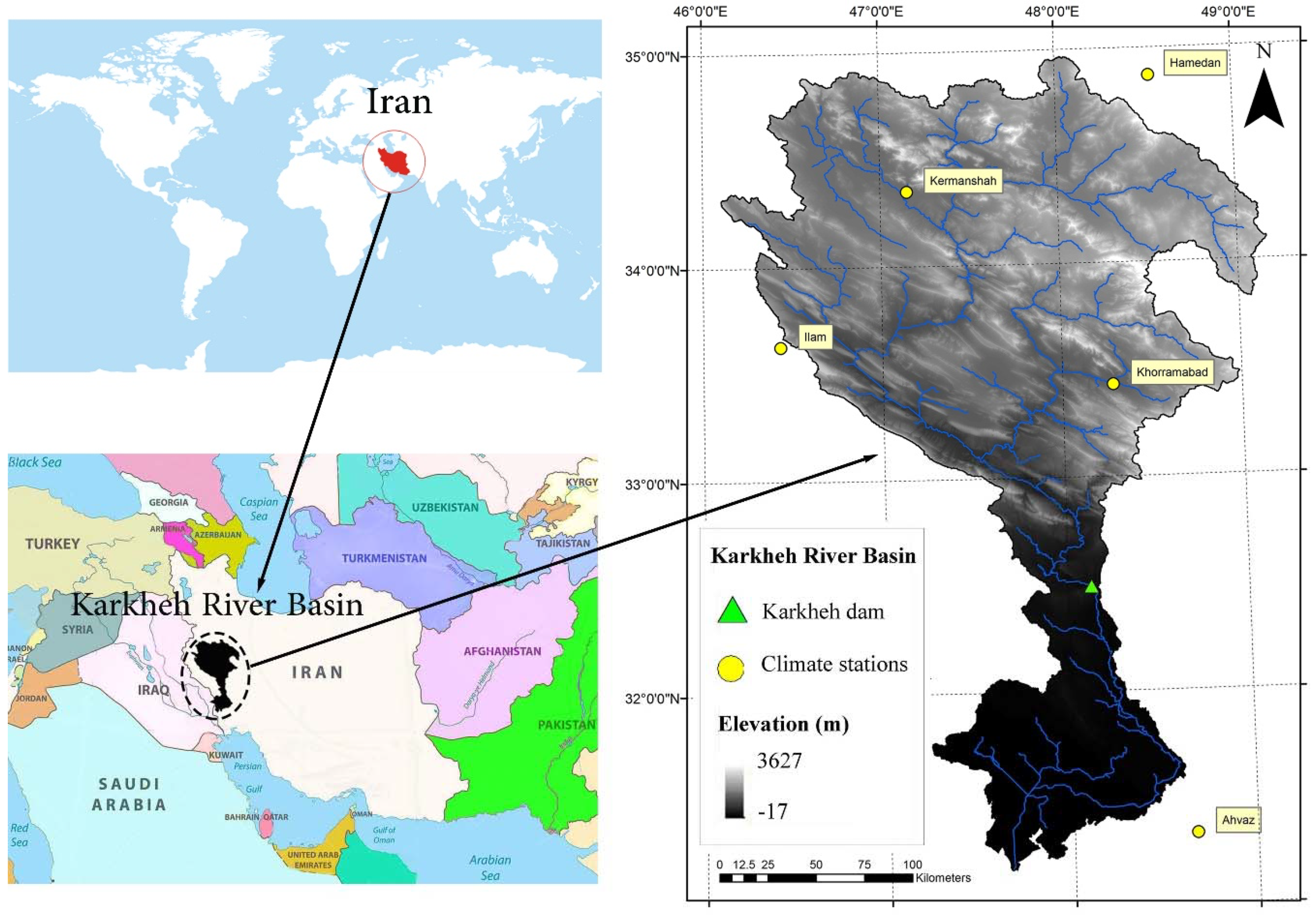
2.1. Study Area and Ground-Based Data Collection

The study area, KRB, is located in south-west Iran between 30°58–34°56 N latitude and 46°06–49°10 E longitude (Figure 1). KRB is about 51,000 km2 in size and contains a relatively flat topography (i.e., <100 m) in its southern- and mountainous areas of the Zagros of up to 3600 m a.s.l. (meters above sea level) in the northern parts.
The climate of the basin is mainly characterized by Mediterranean climate conditions with annual rainfall varying from 150 to 250 mm in the flat south and from 550 to 750 mm in the mountainous north [42,43].
In the middle and upper reaches, the coldest month of the year, January, experiences a mean temperature of −2 °C, and the warmest month, August, of 29 °C. In the lower regions of the KRB, the annual mean temperature fluctuates from 3 °C to 9 °C during wintertime and 36 °C to 41 °C in summertime [44].
Climatological data for daily precipitation, maximum and minimum air temperature from 5 weather stations (Table 1) for the time period January 2003–October 2006—the time interval with the least number of gaps for all stations—were obtained from the Iran Meteorology Department.

2.2. Advanced Microwave Scanning Radiometer–Earth Observing System (AMSR–E) Soil Moisture Product Data

The Advanced Microwave Scanning Radiometer (AMSR–E) on board of NASA’s Aqua satellite was a passive microwave radiometer observing brightness temperatures at six different frequencies, ranging from 6.9 to 89.0 GHz since May 2002, with daily ascending (13:30 equatorial local crossing time) and descending (01:30 equatorial local crossing time) overpasses, over a swath width of 1445 km. It stopped producing data in October 2011 after more than 9 years’ observation, due to some technical problems with the antenna. Several algorithms are applied to retrieve soil moisture products from AMSR–E. In this study, the daily soil moisture data based on the National Aeronautics and Space Administration (NASA) algorithm [45,46] are derived directly from gridded Level-3 land surface product (AE_Land3) for the same time period as for the ground-based climate data above (January 2003–October 2006).

2.3. SM2RAIN Algorithm

Based on the land phase of hydrological cycle, the spatial distribution of rainfall p ( t ) across a watershed at each time step is calculated from the classical, rearranged water balance equation:
  p ( t ) = n Z d s ( t ) / d t + q ( t ) + e ( t ) + g ( t )  
where n [-] is the soil porosity, Z [L] is the soil layer depth, s ( t ) [-] is the relative soil moisture, t [T] is the time and p , q , e and g [L/T] are the precipitation, surface runoff, evapotranspiration, and drainage rate, respectively. By solving this equation and knowing all other components of the hydrological cycle, the rainfall for each time step can be estimated from soil moisture data [25,26]. It should be noted that, as shown by [47], the surface runoff q can assumed to be negligible.
  g ( t ) = a   s ( t ) b  
The drainage rate g ( t ) is estimated with the following equation [48]. The actual evapotranspiration rate e ( t ) is represented by a product of the potential evapotranspiration E T p ( t ) and the relative soil moisture s ( t ) (e.g., [27]):
  e ( t ) = E T p ( t ) × s ( t )  
where E T p ( t ) is calculated by means of the theoretical Blaney and Criddle approach as modified by [49]:
  E T p ( t ) = 2 + c [ ξ ( 0.46 T a ( t ) + 8.13 ) ]  
where T a [C0] is the mean air temperature, ξ is the fraction of daytime hours for the time step used (daily time step in this study) in the total daytime hours of the year, and c is a parameter—to be determined in the calibration process further down—that depends on the daytime wind speed, minimum relative humidity and actual insolation time. Although a value of c = 1.26 has been proposed for this parameter in many studies (see e.g., [49]), it will be further optimized in the calibration/validation process within an acceptable range (0.8–2.1). The parameter values in Equations (2)–(4) ( n Z , a , b , and c ) are calibrated for reproducing observed rainfall data.

2.4. Artificial Neural Network (ANN)

2.4.1. ANN-Basics and Classification

An artificial neural network (ANN) is a computational approach that has been widely used since the 1990’s in various fields of science, involving function estimation, time series forecasting (e.g., [50]) and classification purposes ([51]). The major advantage of using an ANN model instead of deterministic modeling is that the former allows the determination of complicated nonlinear function relationships between some input (action) variables and output (reaction) variables for which the physics is not known a priori. For further details on the concepts and methodology of ANN the reader is referred to the seminal book of [52]. Neural networks can be categorized as either static or dynamic. In a static (feedforward) network the information moves in only one direction from the input to the output (target), irrespective of time, so that there is no feedback from (previous) values of the input and/or output signal. In contrast, in a dynamic network [53] output (target) depends on values of the input and/or output at previous times, i.e., reflecting some kind of inherent memory in the series, as is prevalent in many scientific fields, namely hydrology and meteorology [54] and often described by some autocorrelation. More specifically, dynamic neural networks can then be further divided into time-delay networks (output depends on previous values of input) and feedback (recurrent) (output depends on previous values of output) networks [55,56]. Dynamic neural networks are particularly suitable for nonlinear dynamic systems modeling and have been used in many applications involving time series modeling and prediction.

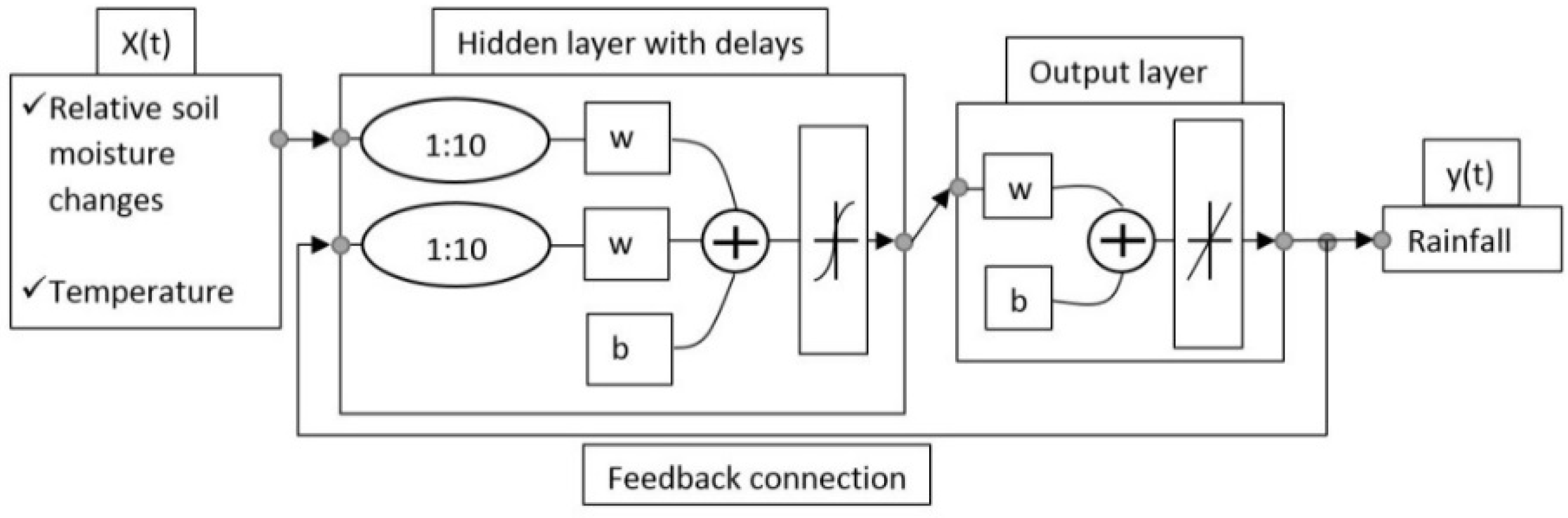
2.4.2. Nonlinear Autoregressive Neural Network with Exogenous Inputs (NARX)

The nonlinear autoregressive network with exogenous inputs (NARX) is an important class of a dynamic network which encompasses the two features above, i.e., a time-delayed nonlinear input (x)–output (y) relationship (NX) and the auto-regressive properties of the output Y (AR) [39,56,57]. The general input-output formulation of a NARX model is as follows:
  y ( t ) = f ( y ( t 1 ) , y ( t 2 ) , , y ( t d ) , x ( t 1 ) , x ( t 2 ) , , x ( t d ) ) + ϵ ( t ) ,    
i.e., predicted values of the dependent variable y(t) at time t is regressed on given d past values of series y and up to d previous values of an independent (exogenous) input signal x(t).
The process of the NARX-network training is usually performed in open-loop form, using known historical values of the input x, i.e., relative soil moisture changes and air temperatures, and output y, i.e., rainfall (see Figure 2, upper panel) and in closed-loop form for subsequent multistep-ahead prediction of y (see Figure 2, lower panel).
The weight values (w) constrain how input data (relative soil moisture, temperature) are related to output data (rainfall). Similarly, bias values (b) are added to the sums calculated in the intermediate and output layers of the network. These values increase the capacity of the network to solve problems by allowing the hyperplanes that separate individual classes to be offset for superior positioning [58]. In order to obtain an accurate prediction model, speed up the calculation and to avoid overfitting, it is important to adjust the maximum number of delays d in Equation (5). Both the SM2RAIN and the NARX neural network are implemented within the MATLAB© environment [59].

2.5. Precipitation Estimates from Remotely Sensed Information Using Artificial Neural Networks Climate Data Record (PERSIANN–CDR)

PERSIANN–CDR (Precipitation Estimates from Remotely Sensed Information using Artificial Neural Networks–Climate Data Record) is a satellite-based precipitation dataset at a resolution of 0.25° × 0.25° for the latitude band 60 N–60 S on the daily scale over the period of 1 January 1983 to present, i.e., is a product with a long-term, global coverage useful for meteorological studies and water resource assessments. The PERSIANN algorithm employs an artificial neural network model to convert the infrared brightness temperatures information into rain rates [21,60]. The daily PERSIANN–CDR product is available to the public and can be downloaded from NOAA’s National Centers for Environmental Information website [61].

3. Results and Discussion

As mentioned in the introduction, two different approaches of daily rainfall estimation in the KRB, i.e., (1) the SM2RAIN algorithm incorporating soil moisture observations from AMSR–E and (2) the NARX neural network algorithm also employing AMSR–E soil moisture observations and ground-based mean air temperature as input and gauge-measured rainfall as output are used and compared to each other.

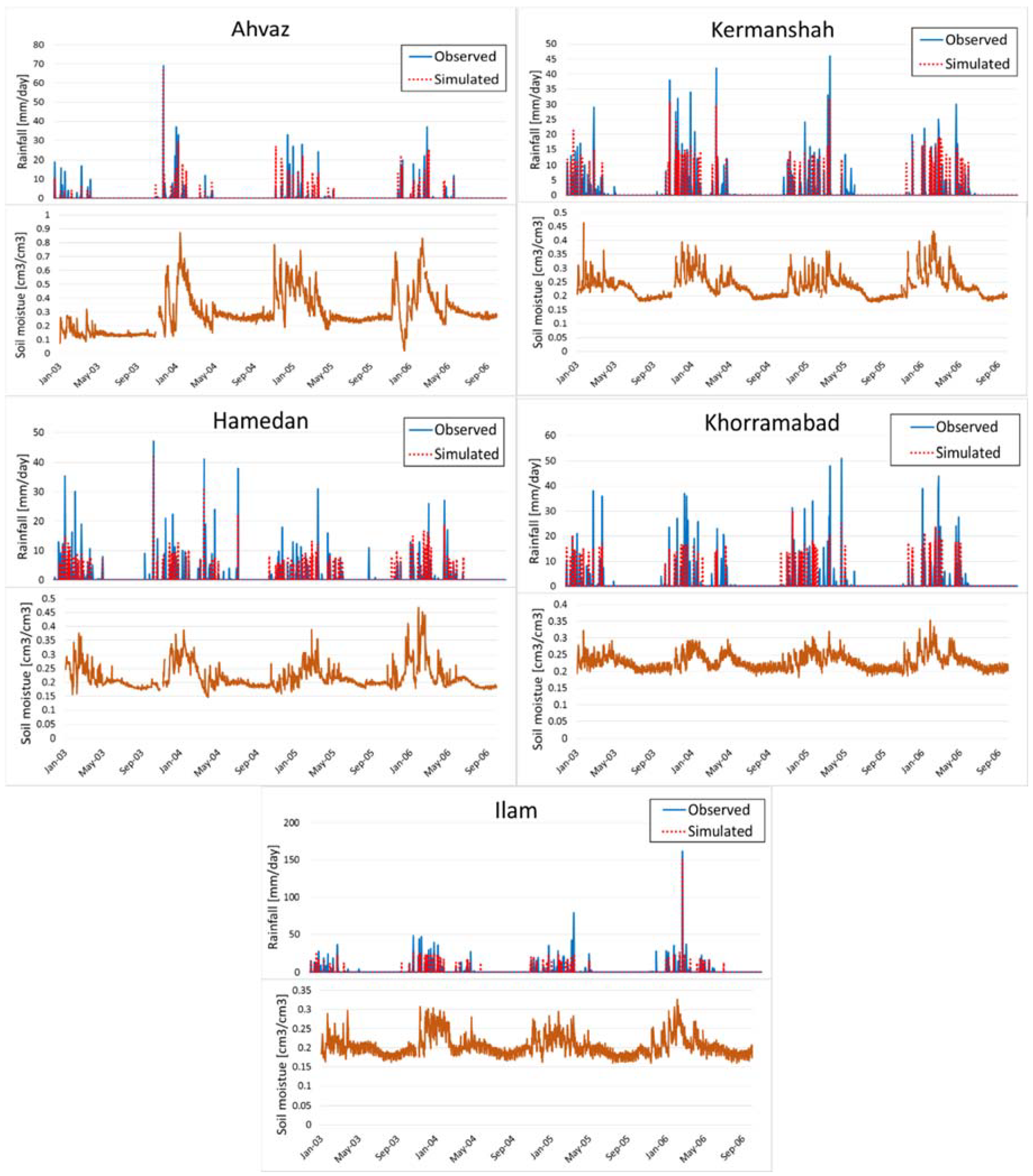
3.1. SM2RAIN Rainfall Estimation Using AMSR–E Soil Moisture Data

The SM2RAIN model is calibrated using AMSRE soil moisture and gauge rainfall data for the period 1 January 2003 to 31 December 2005 and validated with data for the remaining 9 months from 1 January 2006 to 30 September 2006. The calibration is performed as an iterative process whereby the free parameters in the SM2RAIN algorithm (Equations (1)–(4)) are adjusted within their allowable ranges, until the estimated rainfall values are in line with the measured ones, using the coefficient of determination (R2) and the root-mean-square error (RMSE) as quantitative statistical measures.
Time series of the daily SM2R-AMSRE- estimated and observed rainfall for the different stations are shown in the upper panels of Figure 3, with the AMSR–E soil moisture time series depicted in the corresponding lower panels. Table 2 lists the R and root-mean-square error (RMSE) values of the SM2RAIN model fits obtained for the 5 KRB climate stations for both the calibration and validation periods. One may notice from the table that the observed rainfall data are reproduced with reasonable accuracy. In the validation period, the R2-values range between 0.33 for Khorramabad to 0.65 for Ilam. The RMSE is the lowest for Ahvaz station, in accordance with the better R2-value there. Lower performances are also acquired for Ilam and Khorramabad stations, most likely due to the presence of more noise in the associated satellite soil moisture data (see Figure 3).
Besides, surface conditions and topography of the climate stations affect the outcome as well. Thus, the high altitude stations Ilam and Khorramabad stations in the mountainous regions, with more snow cover and frozen soils, do worse than the low altitude station Ahvaz.
Comparisons between the gauge-measured and SM2R-AMSRE estimated rainfall show that the SM2RAIN underestimates the total rainfall amount at all sites. The major reason for this is the constant values of soil moisture for any rainfall amount after reaching saturation [25,47,62,63].
This issue could also explain the reason why at the high-altitude stations, which experience more large rainfall events, the RMSEs are higher. The optimized values of the four parameters (after calibration/validation) that control the water cycle in SM2RAIN method (see Equations (1)–(3)) are listed in Table 3.
Similar to [25,47], the values of these parameters are consistent with their expected physical ones.

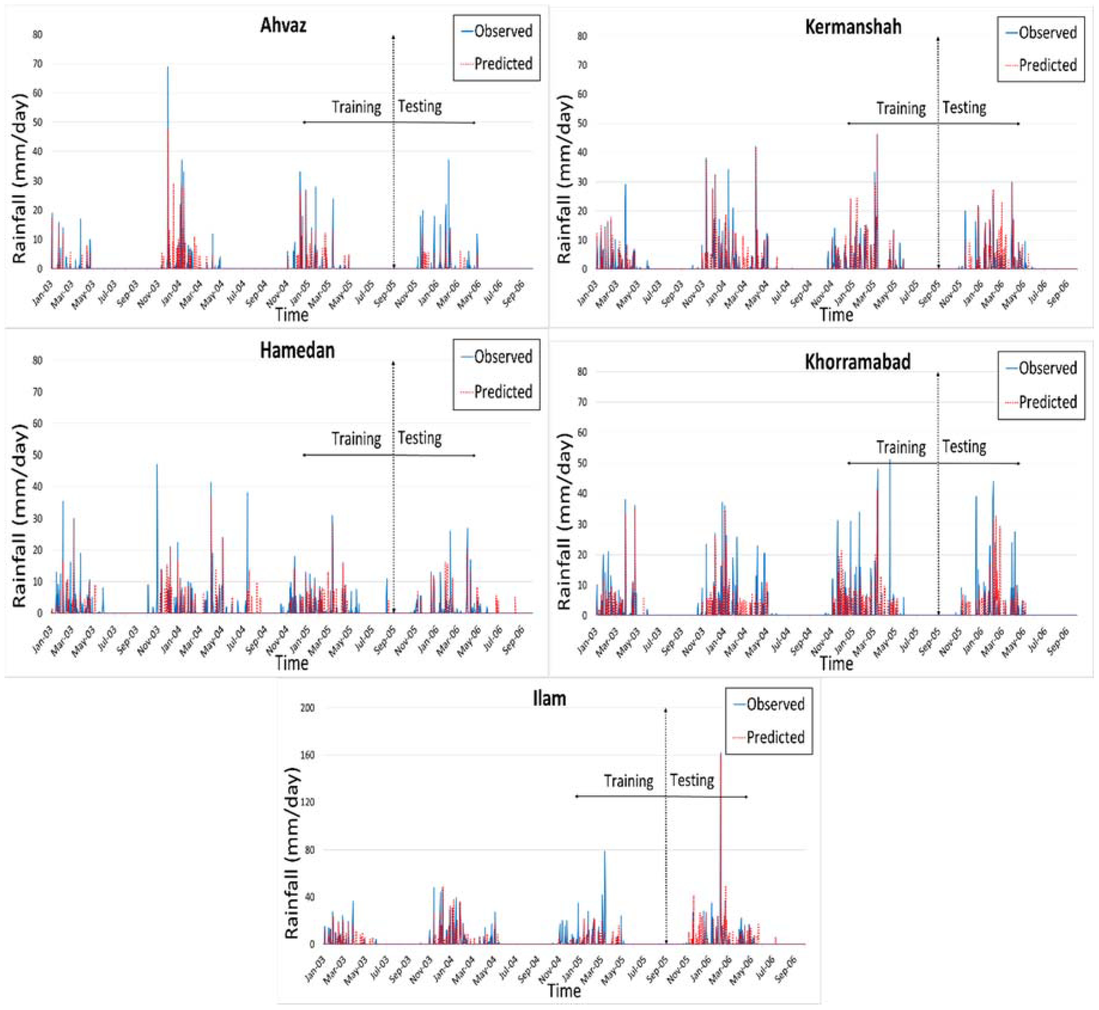
3.2. Rainfall Estimation Using the Nonlinear Autoregressive Network with Exogenous Inputs (NARX) Neural Network

Using AMSR–E satellite data for soil moisture, ground-measured temperatures and rainfall as input (open-loop, see Figure 2) and output, the new NARX neural forecasting model was trained iteratively for the time period January 2003 to September 2005, by adjusting the number of hidden neurons and delays for each KRB station, until a minimal RMSE was obtained. The subsequent testing was performed in closed-loop setup with data in the period September 2005 to September 2006. As mentioned, the application of the NARX model requires the tuning of parameters of the neural network. Table 4 presents the optimal number of hidden neurons and delays d (Equation (5)) found after some lengthy trial-and-error runs to get the best results in terms of the least RMSE.
Using the parameters of Table 4, Figure 4 shows the average NARX-estimated daily rainfall for the training and testing periods for the 5 KRB stations.
Furthermore, the training and one-year prediction accuracies of the NARX model were evaluated by the coefficient of determination (R2), Nash–Sutcliffe efficiency (NSE) and the RMSE, both of which are listed in Table 5. Similar to the results of the SM2RAIN method in the previous section, the best and worst NARX model performances are obtained for stations Ahvaz and Khorramabad, respectively, with R2-values ranging between 0.57 for the former and 0.17 for latter in the testing phase.

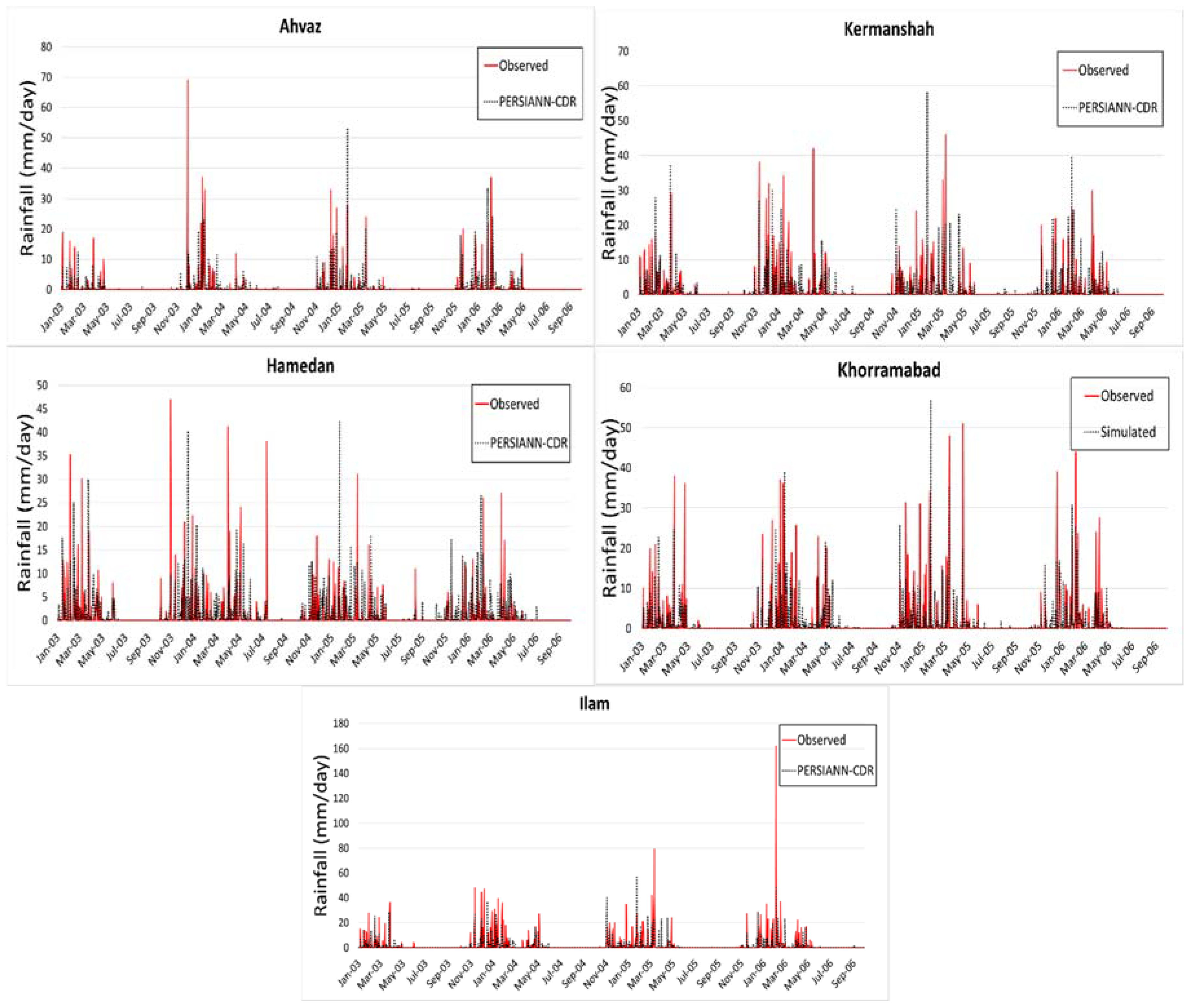
3.3. PERSIANN–CDR Satellite-Based Rainfall

Besides the SM2RAIN- and NARX-estimated rainfalls, the PERSIANN–CDR satellite-based rainfall is also compared with the observed rainfall at the five climate stations in the KRB (see Figure 5).
The PERSIANN–CDR product statistical performances for detecting the observed rainfall are displayed in Table 6.
The best results are achieved for Ahvaz station, followed by Hamedan station, however, with values of R2 and NSE, substantially lower (RMSE higher) than those obtained with the SM2RAIN- (Table 2) and NARX- (Table 5) models. The reason of that somewhat disappointing performance of the PERSIANN–CDR product could be the lack of training of the neural network parameters (over Iran), due to the limited gauge information [64,65], and the low quality of the longwave infrared (IR)-based precipitation estimates [64,66]. Moreover, as can be seen from Figure 5, PERSIANN–CDR tends to underestimate the rainfall at all stations, particularly, for heavy rainfall events.

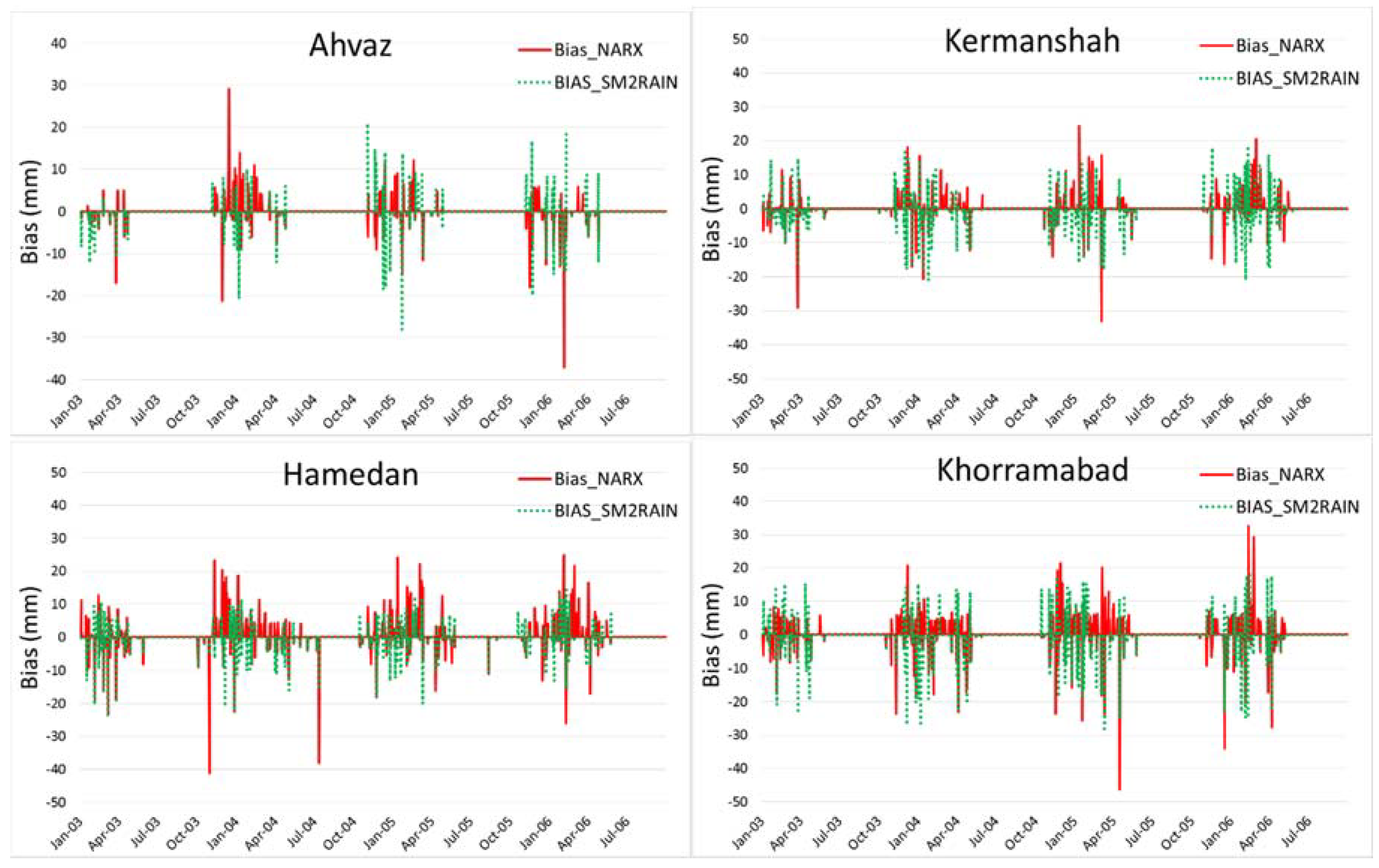
3.4. Comparison of SM2RAIN- and NARX-Simulated Rainfall

Comparison of the rainfall series predicted by NARX (Figure 4) with those of SM2RAIN (Figure 3) as well as of the corresponding statistical performance indicators (Table 3 and Table 5) shows that for climate stations Ahvaz and Kermanshah the simulated NARX-predicted rainfall has a higher correlation with the observed one than the SM2RAIN-predicted one, and this holds for both training/calibration and testing/validation phases/periods.
For station Hamedan, NARX provides almost the same, or even little better results than SM2RAIN. In contrast, for Khorramabad and Ilam stations, SM2RAIN is generally superior by delivering a higher correlation than NARX for all periods/phases. A more revealing picture of the performance differences between the two methods is provided by the plots of the biases, i.e., the absolute differences between the simulated and observed rainfalls for the KRB stations in Figure 6. As can be clearly seen, the SM2RAIN model has for all stations generally less bias, i.e., also less RMSE (see Table 2 and Table 5) than the NARX model. Moreover, as mentioned earlier, SM2RAIN has a tendency to underestimate higher rainfall rates due to saturation and this is the reason why many of the SM2RAIN biases are negative, whereas the NARX bias show more temporary systematic over/under prediction of the rainfall. In any case, these results indicate that a physically based model (SM2RAIN) is—at least in this application—indeed superior to a non-physical neural network model (NARX).

4. Conclusions

In this study, the recently developed SM2RAIN algorithm [26] and a new NARX neural network model are applied to convert AMSR–E soil moisture data to predict daily rainfall at 5 climate stations in the KRB, Iran, which has been a major study region of the authors for some time. The results show that SM2RAIN is able to predict the rainfall at the KRB stations located in different climate regions—from the mountainous north to the flat south of KRB—with varying reliability. Thus, the SM2RAIN-simulated rainfall shows good correlations with the observed one, with R2-values ranging from 0.32 to 0.79 during the calibration and validation period.
The new NARX neural network developed here turns out to be fast and robust and is able to also approximate the daily rainfall data at the same KRB stations in an acceptable manner, whereby the R2 values range between 0.17 and 0.65 for the testing period. From the time series of the biases obtained with the two prediction methods (Figure 5), it can be inferred that although SM2RAIN underestimates daily rainfall in many cases, this method works somewhat better than NARX which produces higher biases and RMSE (Table 2 and Table 5) at all stations. Whether this holds generally, or only in the present KRB application, is yet to be investigated. However, given that SM2RAIN is a physical model its slight superiority may be of no surprise. On the other hand, the appealing feature of the NARX network is that, thanks to the use of exogenous (external) input data, its network complexity is reduced compared with classical multilayer perceptron neural networks. For an additional independent check of the observed rainfall, the PERSIANN–CDR rainfall product has also been applied, but it shows a lower performance than the SM2RAIN and NARX models.
In conclusion, the results of the present study indicate that both SM2RAIN- and NARX models, using AMSR–E satellite soil moisture products, have a high potential for real-time rainfall prediction, but should be further applied with other satellite soil moisture data sets to more catchments worldwide with different physiographic characteristics in order to better assess their practical usefulness.

Author Contributions

M.F. completed the analysis and wrote the manuscript. M.K. supervised the analysis, assisted in the writing of the manuscript, and did the final editing.

Funding

This work was supported by Deutscher AkademischerAustausch Dienst (DAAD) via the PhD/grant ref. no: 91549378.

Conflicts of Interest

The authors declare no conflict of interest.

References

  1. Asante, K.O.; Macuacua, R.D.; Artan, G.A.; Lietzow, R.W.; Verdin, J.P. Developing a Flood Monitoring System From Remotely Sensed Data for the Limpopo Basin. IEEE Trans. Geosci. Remote Sens. 2007, 45, 1709–1714. [Google Scholar] [CrossRef]
  2. Vrochidou, A.-E.K.; Tsanis, I.K.; Grillakis, M.G.; Koutroulis, A.G. The impact of climate change on hydrometeorological droughts at a basin scale. J. Hydrol. 2013, 476, 290–301. [Google Scholar] [CrossRef]
  3. Apurv, T.; Mehrotra, R.; Sharma, A.; Goyal, M.K.; Dutta, S. Impact of climate change on floods in the Brahmaputra basin using CMIP5 decadal predictions. J. Hydrol. 2015, 527, 281–291. [Google Scholar] [CrossRef]
  4. Rossi, M.; Kirschbaum, D.; Valigi, D.; Mondini, A.; Guzzetti, F. Comparison of Satellite Rainfall Estimates and Rain Gauge Measurements in Italy, and Impact on Landslide Modeling. Climate 2017, 5, 90. [Google Scholar] [CrossRef]
  5. Kidd, C.; Bauer, P.; Turk, J.; Huffman, G.J.; Joyce, R.; Hsu, K.-L.; Braithwaite, D. Intercomparison of High-Resolution Precipitation Products over Northwest Europe. J. Hydrometeorol. 2012, 13, 67–83. [Google Scholar] [CrossRef]
  6. Rudolf, B.; Schneider, U. Calculation of gridded precipitation data for the global land-surface using in-situ gauge observations. In Proceedings of the Second Workshop of the International Precipitation Working Group, Moterey, CA, USA, 25–28 October 2004; pp. 231–247. [Google Scholar]
  7. Yilmaz, K.K.; Hogue, T.S.; Hsu, K.-L.; Sorooshian, S.; Gupta, H.V.; Wagener, T. Intercomparison of Rain Gauge, Radar, and Satellite-Based Precipitation Estimates with Emphasis on Hydrologic Forecasting. J. Hydrometeorol. 2005, 6, 497–517. [Google Scholar] [CrossRef]
  8. Tian, Y.; Peters-Lidard, C.D. A global map of uncertainties in satellite-based precipitation measurements. Geophys. Res. Lett. 2010, 37, L24407. [Google Scholar] [CrossRef]
  9. Woldemeskel, F.M.; Sivakumar, B.; Sharma, A. Merging gauge and satellite rainfall with specification of associated uncertainty across Australia. J. Hydrol. 2013, 499, 167–176. [Google Scholar] [CrossRef]
  10. Kurtzman, D.; Navon, S.; Morin, E. Improving interpolation of daily precipitation for hydrologic modelling: Spatial patterns of preferred interpolators. Hydrol. Process. 2009, 23, 3281–3291. [Google Scholar] [CrossRef]
  11. Verworn, A.; Haberlandt, U. Spatial interpolation of hourly rainfall—Effect of additional information, variogram inference and storm properties. Hydrol. Earth Syst. Sci. 2011, 15, 569–584. [Google Scholar] [CrossRef] [Green Version]
  12. Rogelis, M.C.; Werner, M.G.F. Spatial Interpolation for Real-Time Rainfall Field Estimation in Areas with Complex Topography. J. Hydrometeorol. 2013, 14, 85–104. [Google Scholar] [CrossRef]
  13. Stisen, S.; Tumbo, M. Interpolation of daily raingauge data for hydrological modelling in data sparse regions using pattern information from satellite data. Hydrol. Sci. J. 2015, 60, 1911–1926. [Google Scholar] [CrossRef]
  14. Chen, T.; Ren, L.; Yuan, F.; Yang, X.; Jiang, S.; Tang, T.; Liu, Y.; Zhao, C.; Zhang, L. Comparison of Spatial Interpolation Schemes for Rainfall Data and Application in Hydrological Modeling. Water 2017, 9, 342. [Google Scholar] [CrossRef]
  15. Zambrano-Bigiarini, M.; Nauditt, A.; Birkel, C.; Verbist, K.; Ribbe, L. Temporal and spatial evaluation of satellite-based rainfall estimates across the complex topographical and climatic gradients of Chile. Hydrol. Earth Syst. Sci. 2017, 21, 1295–1320. [Google Scholar] [CrossRef] [Green Version]
  16. Bowman, K.P. Comparison of TRMM Precipitation Retrievals with Rain Gauge Data from Ocean Buoys. J. Clim. 2005, 18, 178–190. [Google Scholar] [CrossRef] [Green Version]
  17. Lo Conti, F.; Hsu, K.-L.; Noto, L.V.; Sorooshian, S. Evaluation and comparison of satellite precipitation estimates with reference to a local area in the Mediterranean Sea. Atmos. Res. 2014, 138, 189–204. [Google Scholar] [CrossRef]
  18. Stampoulis, D.; Anagnostou, E.N.; Nikolopoulos, E.I. Assessment of High-Resolution Satellite-Based Rainfall Estimates over the Mediterranean during Heavy Precipitation Events. J. Hydrometeorol. 2013, 14, 1500–1514. [Google Scholar] [CrossRef]
  19. Bayissa, Y.; Tadesse, T.; Demisse, G.; Shiferaw, A. Evaluation of Satellite-Based Rainfall Estimates and Application to Monitor Meteorological Drought for the Upper Blue Nile Basin, Ethiopia. Remote Sens. 2017, 9, 669. [Google Scholar] [CrossRef]
  20. Hughes, D.A. Comparison of satellite rainfall data with observations from gauging station networks. J. Hydrol. 2006, 327, 399–410. [Google Scholar] [CrossRef]
  21. Hsu, K.L.; Gao, X.; Sorooshian, S.; Gupta, H.V. Precipitation Estimation from Remotely Sensed Information Using Artificial Neural Networks. J. Appl. Meteorol. 1997, 36, 1176–1190. [Google Scholar] [CrossRef]
  22. Sorooshian, S.; Hsu, K.-L.; Gao, X.; Gupta, H.V.; Imam, B.; Braithwaite, D. Evaluation of PERSIANN System Satellite–Based Estimates of Tropical Rainfall. Bull. Am. Meteorol. Soc. 2000, 81, 2035–2046. [Google Scholar] [CrossRef] [Green Version]
  23. Kidd, C.; Kniveton, D.R.; Todd, M.C.; Bellerby, T.J. Satellite Rainfall Estimation Using Combined Passive Microwave and Infrared Algorithms. J. Hydrometeorol. 2003, 4, 1088–1104. [Google Scholar] [CrossRef]
  24. Su, J.; Lü, H.; Wang, J.; Sadeghi, A.; Zhu, Y. Evaluating the Applicability of Four Latest Satellite–Gauge Combined Precipitation Estimates for Extreme Precipitation and Streamflow Predictions over the Upper Yellow River Basins in China. Remote Sens. 2017, 9, 1176. [Google Scholar] [CrossRef]
  25. Brocca, L.; Moramarco, T.; Melone, F.; Wagner, W. A new method for rainfall estimation through soil moisture observations. Geophys. Res. Lett. 2013, 40, 853–858. [Google Scholar] [CrossRef] [Green Version]
  26. Brocca, L.; Ciabatta, L.; Massari, C.; Moramarco, T.; Hahn, S.; Hasenauer, S.; Kidd, R.; Dorigo, W.; Wagner, W.; Levizzani, V. Soil as a natural rain gauge: Estimating global rainfall from satellite soil moisture data. J. Geophys. Res. Atmos. 2014, 119, 5128–5141. [Google Scholar] [CrossRef] [Green Version]
  27. Brocca, L.; Camici, S.; Melone, F.; Moramarco, T.; Martínez-Fernández, J.; Didon-Lescot, J.-F.; Morbidelli, R. Improving the representation of soil moisture by using a semi-analytical infiltration model. Hydrol. Process. 2014, 28, 2103–2115. [Google Scholar] [CrossRef]
  28. Ciabatta, L.; Brocca, L.; Moramarco, T.; Wagner, W. Comparison of Different Satellite Rainfall Products over the Italian Territory. In Engineering Geology for Society and Territory; Lollino, G., Arattano, M., Rinaldi, M., Giustolisi, O., Marechal, J.-C., Grant, G.E., Eds.; Springer International Publishing: Cham, Switzerland; Heidelberg, Germany, 2015; pp. 623–626. [Google Scholar]
  29. Fereidoon, M.; Koch, M. SWAT-MODSIM-PSO optimization of multi-crop planning in the Karkheh River Basin, Iran, under the impacts of climate change. Sci. Total Environ. 2018, 630, 502–516. [Google Scholar] [CrossRef] [PubMed]
  30. Ciabatta, L.; Brocca, L.; Massari, C.; Moramarco, T.; Gabellani, S.; Puca, S.; Wagner, W. Rainfall-runoff modelling by using SM2RAIN-derived and state-of-the-art satellite rainfall products over Italy. Int. J. Appl. Earth Obs. Geoinf. 2016, 48, 163–173. [Google Scholar] [CrossRef]
  31. Massari, C.; Brocca, L.; Moramarco, T.; Tramblay, Y.; Didon Lescot, J.-F. Potential of soil moisture observations in flood modelling: Estimating initial conditions and correcting rainfall. Adv. Water Resour. 2014, 74, 44–53. [Google Scholar] [CrossRef]
  32. Wu, C.L.; Chau, K.W.; Fan, C. Prediction of rainfall time series using modular artificial neural networks coupled with data-preprocessing techniques. J. Hydrol. 2010, 389, 146–167. [Google Scholar] [CrossRef] [Green Version]
  33. Philip, N.S.; Joseph, K.B. A neural network tool for analyzing trends in rainfall. Comput. Geosci. 2003, 29, 215–223. [Google Scholar] [CrossRef]
  34. Chattopadhyay, S.; Chattopadhyay, G. Comparative study among different neural net learning algorithms applied to rainfall time series. Meteorol. Appl. 2008, 15, 273–280. [Google Scholar] [CrossRef] [Green Version]
  35. Shukla, R.P.; Tripathi, K.C.; Pandey, A.C.; Das, I.M.L. Prediction of Indian summer monsoon rainfall using Niño indices: A neural network approach. Atmos. Res. 2011, 102, 99–109. [Google Scholar] [CrossRef]
  36. Nastos, P.T.; Moustris, K.P.; Larissi, I.K.; Paliatsos, A.G. Rain intensity forecast using Artificial Neural Networks in Athens, Greece. Atmos. Res. 2013, 119, 153–160. [Google Scholar] [CrossRef]
  37. Abbot, J.; Marohasy, J. Input selection and optimisation for monthly rainfall forecasting in Queensland, Australia, using artificial neural networks. Atmos. Res. 2014, 138, 166–178. [Google Scholar] [CrossRef]
  38. Leontaritis, I.J.; Billings, S.A. Input-output parametric models for non-linear systems Part I: Deterministic non-linear systems. Int. J. Control 1985, 41, 303–328. [Google Scholar] [CrossRef]
  39. Lin, T.; Horne, B.G.; Tino, P.; Giles, C.L. Learning long-term dependencies in NARX recurrent neural networks. IEEE Trans. Neural Netw. 1996, 7, 1329–1338. [Google Scholar] [PubMed] [Green Version]
  40. Boussaada, Z.; Curea, O.; Remaci, A.; Camblong, H.; Mrabet Bellaaj, N. A Nonlinear Autoregressive Exogenous (NARX) Neural Network Model for the Prediction of the Daily Direct Solar Radiation. Energies 2018, 11, 620. [Google Scholar] [CrossRef]
  41. Wunsch, A.; Liesch, T.; Broda, S. Forecasting groundwater levels using nonlinear autoregressive networks with exogenous input (NARX). J. Hydrol. 2018. [Google Scholar] [CrossRef]
  42. Fereidoon, M.; Koch, M.; Brocca, L. Predicting rainfall and runoff through satellite soil moisture data and SWAT modelling for a poorly gauged basin in Iran. J. Hydrol. 2018. (under review). [Google Scholar]
  43. Ahmad, M.-U.-D.; Giordano, M. The Karkheh River basin: The food basket of Iran under pressure. Water Int. 2010, 35, 522–544. [Google Scholar] [CrossRef]
  44. Tavakoli, A.R.; Oweis, T.; Ashrafi, S.; Asadi, H.; Siadat, H.; Liaghat, A. Improving Rainwater Productivity with Supplemental Irrigation in Upper Karkheh River Basin of Iran; International Center for Agricultural Research in the Dry Areas (ICARDA): Aleppo, Syria, 2010; 123p. [Google Scholar]
  45. Njoku, E.G.; Jackson, T.J.; Lakshmi, V.; Chan, T.K.; Nghiem, S.V. Soil moisture retrieval from AMSR-E. IEEE Trans. Geosci. Remote Sens. 2003, 41, 215–229. [Google Scholar] [CrossRef]
  46. Jackson, T.J.; Cosh, M.H.; Bindlish, R.; Starks, P.J.; Bosch, D.D.; Seyfried, M.; Goodrich, D.C.; Moran, M.S.; Du, J. Validation of Advanced Microwave Scanning Radiometer Soil Moisture Products. IEEE Trans. Geosci. Remote Sens. 2010, 48, 4256–4272. [Google Scholar] [CrossRef]
  47. Brocca, L.; Massari, C.; Ciabatta, L.; Moramarco, T.; Penna, D.; Zuecco, G.; Pianezzola, L.; Borga, M.; Matgen, P.; Martínez-Fernández, J. Rainfall estimation from in situ soil moisture observations at several sites in Europe: An evaluation of the SM2RAIN algorithm. J. Hydrol. Hydromech. 2015, 63, 201–209. [Google Scholar] [CrossRef]
  48. Famiglietti, J.S.; Wood, E.F. Multiscale modeling of spatially variable water and energy balance processes. Water Resour. Res. 1994, 30, 3061–3078. [Google Scholar] [CrossRef] [Green Version]
  49. Doorenbos, J.; Pruitt, W.O. Background and Development of Methods to Predict Reference Crop Evapotranspiration (ETo); Appendix II in FAO-ID-24; FAO: Rome, Italy, 1977; pp. 108–119. [Google Scholar]
  50. Zare, M.; Koch, M. Using ANN and ANFIS Models for simulating and predicting Groundwater Level Fluctuations in the Miandarband Plain, Iran. In Proceedings of the 4th IAHR Europe Congress. Sustainable Hydraulics in the Era of Global Change, Liege, Belgium, 27–29 July 2016; p. 416. [Google Scholar]
  51. Ince, H. Non-Parametric Regression Methods. Comput. Manag. Sci. 2006, 3, 161–174. [Google Scholar] [CrossRef]
  52. Bishop, C.M. Neural Networks for Pattern Recognition; Clarendon Press: Oxford, UK, 1995. [Google Scholar]
  53. Terzic, E.; Nagarajah, C.R.; Alamgir, M. Capacitive sensor-based fluid level measurement in a dynamic environment using neural network. Eng. Appl. Artif. Intell. 2010, 23, 614–619. [Google Scholar] [CrossRef]
  54. Hung, N.Q.; Babel, M.S.; Weesakul, S.; Tripathi, N.K. An artificial neural network model for rainfall forecasting in Bangkok, Thailand. Hydrol. Earth Syst. Sci. 2009, 13, 1413–1425. [Google Scholar] [CrossRef] [Green Version]
  55. Pearlmutter, B. Dynamic Recurrent Neural Networks; Technical Report CMU-CS-90-196; School of Computer Science, Carnegie Mellon University: Pittsburgh, PA, USA, 1990. [Google Scholar]
  56. Ćirović, V.; Aleksendrić, D.; Mladenović, D. Braking torque control using recurrent neural networks. Proc. Inst. Mech. Eng. Part D 2012, 226, 754–766. [Google Scholar] [CrossRef]
  57. Huo, F.; Poo, A.-N. Nonlinear autoregressive network with exogenous inputs based contour error reduction in CNC machines. Int. J. Mach. Tools Manuf. 2013, 67, 45–52. [Google Scholar] [CrossRef]
  58. Leverington, D. A Basic Introduction to Feedforward Backpropagation Neural Networks; Technical Report; Texas Tech University: Lubbock, TX, USA, 2009; Available online: http://www.webpages.ttu.edu/dleverin/neural_network/neural_networks.html (accessed on 2 July 2018).
  59. Beale, M.H.; Hagan, M.T.; Demuth, H.B. Neural Network Toolbox™ User’s Guide; R2012a; The MathWorks, Inc.: Natick, MA, USA, 2012. [Google Scholar]
  60. Tan, M.L.; Santo, H. Comparison of GPM IMERG, TMPA 3B42 and PERSIANN-CDR satellite precipitation products over Malaysia. Atmos. Res. 2018, 202, 63–76. [Google Scholar] [CrossRef]
  61. PERSIANN-CDR Data Downloads. Available online: https://www.ncdc.noaa.gov/cdr/atmospheric/precipitation-persiann-cdr (accessed on 3 July 2018).
  62. Crow, W.T.; Berg, A.A.; Cosh, M.H.; Loew, A.; Mohanty, B.P.; Panciera, R.; de Rosnay, P.; Ryu, D.; Walker, J.P. Upscaling sparse ground-based soil moisture observations for the validation of coarse-resolution satellite soil moisture products. Rev. Geophys. 2012, 50, 3675. [Google Scholar] [CrossRef]
  63. Chen, F.; Crow, W.T.; Ryu, D. Dual Forcing and State Correction via Soil Moisture Assimilation for Improved Rainfall–Runoff Modeling. J. Hydrometeorol. 2014, 15, 1832–1848. [Google Scholar] [CrossRef]
  64. Yang, Y.; Tang, G.; Lei, X.; Hong, Y.; Yang, N. Can satellite precipitation products estimate probable maximum precipitation: A comparative investigation with gauge data in the Dadu River Basin. Remote Sens. 2018, 10, 41. [Google Scholar] [CrossRef]
  65. Li, Z.; Yang, D.; Hong, Y. Multi-scale evaluation of high-resolution multi-sensor blended global precipitation products over the Yangtze River. J. Hydrol. 2013, 500, 157–169. [Google Scholar] [CrossRef]
  66. Guo, H.; Chen, S.; Bao, A.; Hu, J.; Gebregiorgis, A.S.; Xue, X.; Zhang, X. Inter-comparison of high-resolution satellite precipitation products over central Asia. Remote Sens. 2015, 7, 7181–7211. [Google Scholar] [CrossRef]
Figure 1. Map of the Karkheh river basin with weather stations and the Karkheh dam.
Water 10 00964 g001
Figure 2. Recurrent neural model (nonlinear autoregressive network with exogenous inputs (NARX) network in open-loop (upper panel) and closed-loop (lower panel) architecture according to Beale et al., 2012, with an example of d = 10 delays).
Water 10 00964 g002aWater 10 00964 g002b
Figure 3. Observed and SM2RAIN-estimated rainfall (upper panels) and original Advanced Microwave Scanning Radiometer–Earth Observing System (AMSR–E soil moisture data (lower panels) from January 2003 to October 2006.
Water 10 00964 g003
Figure 4. Observed and NARX model-predicted daily rainfall for the KRB stations for training and testing stages.
Water 10 00964 g004
Figure 5. Observed and Precipitation Estimates from Remotely Sensed Information using Artificial Neural Networks–Climate Data Record (PERSIANN–CDR) satellite-based rainfall for the KRB stations during the period from January 2003 to September 2006.
Water 10 00964 g005
Figure 6. Bias (simulated-observed) of the NARX- and SM2RAIN-modeled rainfall for the 5 KRB stations.
Water 10 00964 g006aWater 10 00964 g006b
Table 1. Geographical characteristics of the selected climate stations.
Climate StationLongitude (°East)Latitude (°North)Elevation (m a.s.l.)
Hamedan48.5334.871741
Kermanshah47.1534.351319
Ilam46.4333.631337
Khorramabad48.2833.431148
Ahvaz48.6731.3322
Table 2. Coefficient of determination (R2), root-mean-square error (RMSE) and Nash–Sutcliffe efficiency (NSE) of SM2RAIN model fit of rainfall at the 5 Karkheh river basin (KRB) climate stations for calibration and validation periods.
Climate StationR2RMSE (mm)NSE
CalValCalValCalVal
Ahvaz0.570.442.52.50.630.36
Kermanshah0.480.233.073.910.550.11
Hamedan0.380.313.060.120.440.09
Khorramabad0.350.334.194.320.380.26
Ilam0.280.655.584.470.330.56
Table 3. Optimized parameter values of the SM2RAIN-Equations (1)–(3) for the 5 KRB climate stations.
Climate StationZn (mm)a (mm/day)bc
Ahvaz32.1392.21.90
Kermanshah34.8502.32.00
Hamedan58.3561.51.20
Khorramabad39.2461.91.95
Ilam44.6872.51.90
Table 4. Optimal number of hidden neurons and delays d for the NARX model at 5 KRB stations.
Climate StationNeuronsDelays
Ahvaz810
Kermanshah108
Hamedan910
Khorramabad1410
Ilam1012
Table 5. Coefficient of determination (R2), root-mean-square error (RMSE) and Nash–Sutcliffe efficiency (NSE) of the NARX-model fits for the 5 KRB climate stations for the training and testing phases.
Climate StationTrainingTesting
R2RMSE (mm)NSER2RMSE (mm)NSE
Ahvaz0.653.30.620.574.80.28
Kermanshah0.604.80.550.376.60.53
Hamedan0.405.80.160.266.80.10
Khorramabad0.375.90.380.177.30.27
Ilam0.326.30.790.238.90.31
Table 6. Coefficient of determination (R2), root-mean-square error (RMSE) and Nash–Sutcliffe efficiency (NSE) for PERSIANN–CDR during the period from January 2003 to September 2006.
Climate StationR2 RMSE (mm)NSE
Ahvaz0.303.240.18
Kermanshah0.293.870.09
Hamedan0.316.030.31
Khorramabad0.274.410.21
Ilam0.124.06−0.26

