Abstract
Numerical modelling is becoming a major tool for supporting environmental studies at different scales, thanks to the ability of up-to-date codes to reproduce the complex mechanisms of the natural environment in quite a reliable manner. In evaluating the habitat diversity of anthropized rivers, however, many issues are rising because of the intrinsic complexity of the physical processes involved and the limitations associated with numerical models. Using a reach of the Po River in Italy as a case study, the present works aims to provide a qualitative description of the changes of the Eco-Environmental Diversity index as a response to different constant flow discharges typically observed along this reach. The goals are achieved by means of two solvers of the freeware iRIC suite, applied in cascade to first simulate the 2D fluvial hydrodynamics and subsequently provide a qualitative estimate of the habitat conditions. Despite the several simplifications intrinsically present in the modelling cascade and the ones introduced for practical purposes, the results show that an extremely strong and long-lasting reduction of the flow discharge, like the one very recently observed, can ultimately threaten the overall biological status of the river. Because of the modelling uncertainties, these preliminary outcomes are only qualitative and show the need for more research, both in terms of data acquisition and numerical schematization, to adequately and quantitatively evaluate the effects of transient hydrology on the river ecosystems. Moreover, additional field surveys are necessary to calibrate and validate the used biological parameters, aiming to obtain sufficiently reliable estimates.
1. Introduction
The response of fluvial ecosystems to external and internal drivers has been a matter of study for more than a century [1,2], and the scientists involved have had very different backgrounds and applied manifold techniques. Research on the responses of river systems to external forcing has considered the influence of single [3], sequential [4,5] and multiple [6] stressors, showing that the cumulative effect produced by the latter is far from being completely understood, especially in large rivers. Given that large watercourses are among the most productive ecosystems worldwide [7], they are also highly affected by anthropogenic activities such as dredging, navigation, river training, bank stabilization or dam construction (see, among others, [2,8,9,10,11,12,13]), involving significant morphological modifications, changes of riparian vegetation and species invasions [14,15,16] acting at manifold scales. Nowadays, the use of numerical models for evaluating the effects of multiple natural and anthropogenic stressors in impacted ecosystems is becoming paramount and widely diffused also because of the improvements in computational capacity. In fact, several modelling tools, both commercial and freeware, are now available and can be applied to evaluate the dynamics of river ecosystems at the appropriate spatial and temporal scales [2,3,17], as well as to assess the benefits deriving from small- and large-scale river restoration projects [18].
To provide additional insights on the use of numerical models in assessing riverine hydrodynamics and habitat conditions, the freeware iRIC (International River Interface Cooperative) suite (i-ric.org/en) was chosen because of its flexibility and the availability of different solvers, which can be combined and were developed for adequately simulating the eco-hydraulics of small and intermediate streams, but also large rivers [19]. As one of the most anthropized watercourses in Italy, the Po River represents a perfect case study for testing the suite and evaluating its ability to numerically reproduce the effects of different hydrological conditions on the Eco-Environmental Diversity (EDD) index. Considering different flow discharges, it is possible to evaluate if the forecasted increase of drought periods [20] can affect the habitat conditions of this Italian watercourse. The EDD index, computed on the basis of Simpson’s diversity index [21], is usually adopted to evaluate fish diversity along watercourses, especially in Japan [22], being one of a series of metrics frequently used to assess the hydraulic and biological characteristics of in-stream habitats that need to be considered for successful stream habitat restoration [23]. Despite using a well-known and tested parametrization, because of the lack of spatially distributed information on fish habitat and the assumptions intrinsically correlated to the numerical codes, the present application represents only a preliminary estimate on EDD index, and is not pretending to propose any quantitative information, but rather to provide a qualitative indication of the habitat conditions along one of the most impacted Italian rivers. It is worth mentioning that, because of the introduced simplifications, the outcomes reported here are site-specific, and can hardly be extended to other watercourses.
After a short description of the study site, the schematization used in the two numerical models will be addressed, pointing out the main simplifications introduced and their impact on the modelling outcomes. Even if based on several schematizations and therefore intrinsically affected by uncertainties, as discussed in the following, the presented results highlight the ability of the iRIC suite to work in a combined way, simulating first the measured fluvial hydrodynamics in a rather good manner when compared with field information, and then the changes of the habitat conditions in terms of the EDD index. Because of a lack of data and the numerous assumptions, however, only qualitative indications on the possible changes of the Po River habitat can be retrieved from the modelling runs. The relationship between the EDD index and the flow discharge can provide additional insights into the possible consequences of the combined impact of climate change and anthropogenic pressure on the future habitat of the Po River.
2. Case Study
The Po River, the longest watercourse in Italy, flows eastward across northern Italy for about 660 km, from the Alps to the Adriatic Sea (Figure 1a). With a drainage area of about 74,000 km², the watershed can be divided into three sectors based on the lithology and the maximum elevation: the Alpine sector of crystalline and carbonate rocks (maximum relief: around 4500 m asl), the Apennine sector, mostly composed of sedimentary rocks with high clay content (maximum relief: around 2000 m asl) and the central alluvial area that includes the Po plain and the Po River delta [24]. The middle and lower portions of the Po River are subjected to high flood hazard and, consequently, have been heavily embanked for decades [25] to protect the highly anthropized surroundings.

Figure 1.
(a) Po River basin; (b) DEM of the studied area, from the upstream end of Borgoforte to the downstream end of Sermide; (c) yearly time series of flow discharge measured between 1986 and 2017 at the gauging station of Borgoforte (Mn).
The annual hydrograph shows two peaks in discharge, normally in autumn and spring, generated by rainfall and snowmelt, respectively. For the period 1924–2009, the long-term mean annual discharge recorded at the Piacenza gauging station was around 1000 m3/s [26], while the total annual sediment and freshwater discharges to the Northern Adriatic Sea were about 13 × 109 kg and 40–50 km3, respectively [27,28].
The iRIC models were applied to a reach of about 70 km between Borgoforte (Mn) and Sermide (Mn). As visible from the 2 m Digital Terrain Model (DTM) provided by the local water authority AIPO (Agenzia Interregionale per il fiume Po, Italy) in 2005 (Figure 1b), this reach has a mean width of 600–800 m, including the floodplains and the emerging bars, characterizing the Po as an intermediate stream. This DTM combines information retrieved by means of LiDAR (data collected using two different laser scanners: 3033 Optech ALTM and Toposys Falcon II), multi-beam sonar survey for the navigable portion and a traditional ground survey of some river cross sections. The bottom slope of the studied reach is in the order of 0.05%.
The present river course has been heavily affected by human interventions during the last century, with evident modifications of the fluvial pattern. Gravel and sand mining from the riverbed, particularly intense during the 1960s, and the creation of river embankments to prevent flooding of the surrounding floodplains, as well as the construction of hydropower dams along the Alpine tributaries, promoted a severe decrease in the sediment load and, consequently, an important degradation of the overall river bed, with an oversimplification of its path [29,30,31]. This long-term anthropogenic pressure altered the overall sediment dynamics, and nowadays the middle reach results in a morphological quasi-equilibrium [9], where the morphology is altered only by extreme events. At present, indeed, the lowland part of the Po River is like a single sandy-bedded canal flowing smoothly between fixed levees and vegetated banks, with a recognizable decrease in the habitat conditions fostered by an overstabilization of banks and bars.
For the present simulations, the hydrological conditions were derived from the analysis of the water discharges measured at the Borgoforte gauging station between 1986 and 2017 (Figure 1c), located at the upstream end of the studied reach. Even if a slight decrease in yearly flow discharge was observed during the studied period, no statistically meaningful trends can be recognized.
3. Numerical Modelling
Several hydraulic models have been used to simulate instream habitat suitability at different temporal and spatial scale [23]. Among others, PHABSIM (Physical Habitat Simulation System) is a well-established hydro-ecological model developed by the United States Geological Survey (www.usgs.gov/software/physical-habitat-simulation-phabsim-software-windows) and provides a suite of tools for the 1D numerical modelling of hydraulic habitat suitability for fish and invertebrate species [32,33]. However, such a schematization can be too crude, given that complex environments require a 2D or even a 3D representation of the flow field [31,34,35]. Therefore, the present application will involve a complete suite composed by a 2D solver for evaluating flow velocities and depths along the Po River, coupled with a 2D tool for estimating the instream habitat suitability at the reach scale.
In the iRIC (International River Interface Cooperative) structure, solvers are kept separate from the interface, communicating with it through a definition file that instructs the interface on how to configure itself for the solver to be used, and a binary data structure that exchanges information [19]. Thus, iRIC is only an interface, which permits to investigate the same case study at different spatial and temporal scales by means of many interacting tools [36]. In particular, the modelling of the habitat diversity along the Po River was performed applying two different solvers of the freeware iRIC suite (i-ric.org/en) in a cascade manner: River2D and DHABSIM. Indeed, the latter solver needs river geometry, flow depth and velocity field as input parameters, which can be derived from the output of the first solver.
3.1. River 2D Solver for the River Hydraulics
The original code River2D is a 2D (depth-averaged) finite-element solver developed at the University of Alberta, Canada [37,38]. A thorough description of its mathematical background can be found in the solver manual [38], so it is not described here for the sake of simplicity, apart from a few characteristics. The original modelling structure was maintained in implementing it in the freeware iRIC solver (i-ric.org/en/solvers/river2d), which adopts a finite-element for solving the depth-averaged de St. Venant equations expressed in a conservative form. The code assumes that the pressure distribution along the vertical is hydrostatic, therefore it is applicable only for lowland reaches where the bed slope changes gently (namely, longitudinal variations of about 10% cannot be correctly modelled), like the presented case study. Moreover, Coriolis and wind forces are assumed to be negligible, as usually made for reproducing relatively short river reaches. The friction slope depends on the bed shear stresses, assumed related to the magnitude and direction of the depth-averaged velocity, and the bed roughness is computed using the White–Colebrook formulation of the Chézy coefficient. As for the depth-averaged transverse turbulent shear stresses, they are modelled following a Boussinesq type eddy viscosity formulation.
The River2D model distributes the flow across the inflow boundary proportional to the depth, resulting in the fastest velocity close to the thalweg. The river region included between the main levees was discretized by means of a triangular irregular network (TIN) grid, with grid elements having a maximum area of 250 m2. In this manner, the whole 70-km domain was covered using around 8 × 10⁵ nodes, having a similar size regardless of being within the main active channel or along the floodplains. The default upwind coefficient (0.5) was used in River2D’s Petrov‒Galerkin finite element scheme [39,40], while the default groundwater parameters (maximum depth = 1 m, transmissivity = 0.1 m2/s, storativity = 1) were accounted for in the wet/dry algorithm, which changes surface flow equations to groundwater flow equations [38]. Such a low value of the transmissivity means that the groundwater discharge can be neglected. The bed roughness was imposed equal to 0.035 s/m1/3 in the main channel and 0.055 s/m1/3 along the floodplains, as calibrated in previous applications [25,38]. This solver uses a non-dimensional Chézy coefficient to close the stress terms, computed as a function of the effective roughness height. Therefore, the flow resistance along the stream is primarily due to the bed material roughness.
Provided that the River2D code simulates only constant discharges as input boundary conditions, six sets of scenarios were simulated for evaluating the possible flow fields associated with typical discharges observed along the stream. Because of these modelling limitations, yearly discharges were assumed to be more representative of the general river behaviour rather than the daily ones. Therefore, three scenarios correspond to the long-term statistics as measured at the gauging station of Borgoforte in the period 1986–2017 (Figure 1c): minimum, mean and maximum yearly discharges of 760 m3/s, 1300 m3/s and 2200 m3/s, respectively. Other scenarios are assumed for covering the whole hydrograph, accounting for extreme events, assuming that they last for a long period: 200 m3/s, 3000 m3/s and 5000 m3/s. As for the downstream conditions, a calibrated depth-unit discharge relationship was adopted, changing the depth-unit discharge parameter K for each simulation to obtain an equilibrium between the discharges entering and going out from the domain. This parameter spans from 0.12 for the case of 200 m3/s to 3.00 in the case of the flooding discharge 5000 m3/s. The exponent m of the depth-unit discharge was imposed equal to 0.5 for all the simulations. The fixed upstream (14.55 m asl) and downstream (5.51 m asl) water elevations were extracted from information retrieved from the local water authority.
The computational time step (maximum Δt = 10 s) is reduced thanks to an adaptive time step, and the overall simulations are quicker with respect to other unstructured grid models [19]. The total simulated time was 1 × 10⁵ s, necessary to stabilize the code avoiding instabilities due to the initial conditions. For the sake of sensitivity, longer and shorter simulations were performed, pointing out that the adopted parameters are corrected, given that the modelling outcomes are indicative of the hydrodynamic behaviour of the reach.
3.2. DHABSIM Solver for the Ecosystem Dynamics
In Japan, where it was first developed, the DHABSIM (Diversity Habitat Simulation) code is frequently adopted to compute the EDD index, in an attempt to quantify the diversity of habitat within a home-range area [39], following an increasing trend of eco-hydrological modelling [41,42]. Recent studies [19] found that this index was positively correlated with fish species richness, and can, therefore, provide a good estimate of the river status.
This 2D solver (i-ric.org/en/solvers/dhabsim) imports geometry, velocity, and depth from other flow calculation solvers implemented in iRIC, like the River2D, and then uses this information to compute the habitat conditions for small to medium-sized rivers without using Habitat Suitability Indices for specific fish species. Such a model cannot, therefore, be applied in large lowland rivers, characterized by high discharges and a very wide (kilometres) main channel.
Based on the diversity-based algorithm and the physical flow inputs, the solver outputs a habitat distribution map. The fish home-range derives from the Minns formula [43], and is computed based on the average fish length:
where Ahr represents the home range (m2) and L the fish length (mm).
The EED index of each point is a combination of geometry, fish preferences on flow field (depth and velocity), sediment composition of the bed and vegetation cover (Equation (2)). This index ranges between 0 and 1, and an increment of 0.1 point means that one species of fish may increase in the target river. In the case of EDD index > 0.8 points, the habitat has good conditions for fish habitat.
where S is the total number of categories i (depth, velocity, bed, vegetation) considered, N is the number of nodes in the home range and ni is the node number of category i. Indeed, the code permits to spatially specify the categories by drawing local regions.
For the present simulation, the grid was directly exported from River2D and has a maximum area of 25 m2, equal to the 1/10 of the home-range and directly computed by the solver [22]. As for the values representing the fish preferences (depth and velocity), they are assumed constant in the whole reach, due to the lack of more detailed information. The ones related to water velocity were derived from the limited literature available [16], while for the depth categorization the default values were maintained because of a lack of specific information. The river bed was considered uniform and constituted by sand. For the sake of simplicity, no vegetation was considered in this preliminary application. On the basis of these simplifications, to simulate the total time t = 1 × 10⁵ s, as derived from the hydrodynamic simulations, a normal desktop PC requires around 12 h for each run.
Aiming to obtain a qualitative analysis of the effects of changing hydrology and because of a lack of specific field information, no sensitivity analysis on the EDD index was performed.
4. Results
The River2D solver was calibrated against measured data [44] and previous numerical simulations [35,45] in terms of (i) water elevation measured by means of a hydrometer at the gauging station of Revere (Figure 1); (ii) velocity field retrieved from an ADCP (Acoustic Current Doppler Profiler) survey performed along a 10-km reach close to Revere. Based on the outcomes of the hydrodynamics solver, the ecosystem dynamics can be computed by applying the DHABSIM solver.
4.1. River Hydrodynamics
For the sake of simplicity and to obtain a preliminary estimate of the flow field, the hydrodynamics of this reach of the Po River were simulated accounting for a fixed bed roughness in the main channel (0.035 s/m1/3) and along the floodplains (0.055 s/m1/3), without accounting for spatially variable patterns possibly related to vegetation or bedforms. Even if based on strong simplifications, the obtained results are in good accordance with previous simulations [36,46] and local field data recently acquired with an ADCP [44], and are therefore considered as representative of the overall hydrodynamics of the reach.
In particular, during mean flow conditions, the flow depth reaches a maximum of around 20 m along the thalweg, while the magnitude of the flow velocities ranges is below 1.5 m/s, comparable with field measurements [44]. It is worth recalling here that such results represent an average over each cell, having a maximum area of around 250 m2, and therefore should be interpreted as a general trend of the overall river behaviour rather than very local estimates.
As visible in Figure 2, where the contours of the velocity fields are reported, in the main channel the higher the discharge, the higher the flow velocity, as one would expect. However, one can also see that, in the case of high water levels (Figure 2a), there are more active channels, especially in the lower part of the studied reach, suggesting that such conditions can be more suitable for the exchange of fluxes between the main channel and the adjacent floodplains. Moreover, as discussed in the following sections, these medium to high flow conditions are paramount for establishing good habitat conditions.
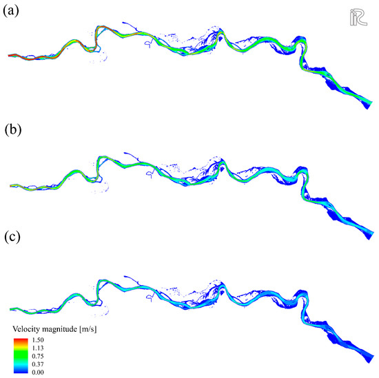
Figure 2.
Simulated velocity profiles for the (a) maximum, (b) mean, and (c) minimum discharge.
In detail, a decrease of the flow velocity is observable going from upstream (Borgoforte) towards downstream (Sermide), because of a reduction of the bed slope and an increase in the river dimensions. Indeed, the first part of the river is quite narrow with a limited number of secondary channels and bars, while the middle part is characterized by several curves and islands, potentially creating a better habitat for the local fish community. The lower portion of the studied reach has a relatively large floodplain, which is also covered by water during low flow conditions (Figure 2c).
The levels in the main channel remain roughly constant along the whole reach, given that channel depth and width are compensating for each other, and therefore the active cross section varies only slightly.
Aiming to evaluate the effects of extreme flood and drought events, two major and one very minor discharges were simulated (Figure 3). As one can see, very high flow discharges involve very high velocity, over 1.5–2.0 m/s along the entire reach (Figure 3a). On the other hand, very low discharges (Figure 3c) involve velocities of maximum 0.4 m/s, which can be detrimental to the fluvial habitat, because prolonged droughts can interrupt the water, sediment and biota continuity, ultimately affecting the overall ecological status of the watercourse.
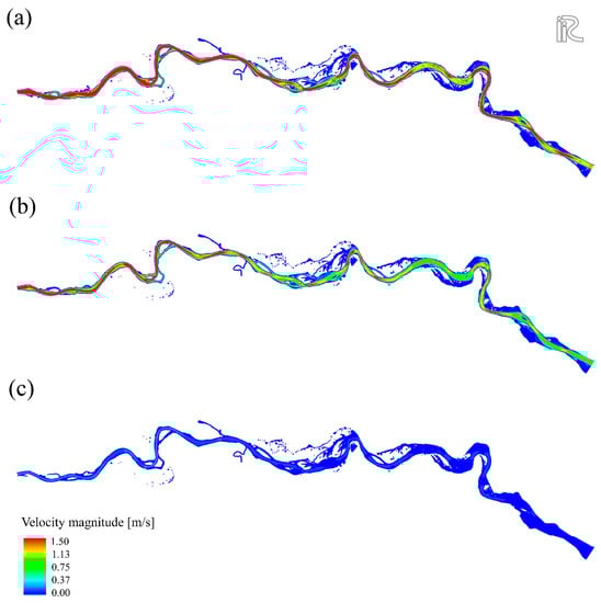
Figure 3.
Simulated velocity profiles for the extreme events: (a) 5000 m3/s, (b) 3000 m3/s, (c) 200 m3/s.
Because the model is a fixed-bed one, only clear water is here considered, without describing the bed morphodynamics. Therefore, one cannot adequately capture the effect of high velocities on the sediment transport and bed morphology, but previous evaluations performed on the middle part of the reach [33,43] have suggested that the river is subject to general erosion and an overall redistribution of sand sediments during floods, with possible consequences for the local habitat. On the other hand, considering the effect of the normal hydrological flow regime on the sediment dynamics, [9] pointed out that, nowadays, the river results in a morphological quasi-equilibrium, which can be altered only in the case of flooding.
4.2. Eco-Environmental Diversity Index
Despite the non-detailed results obtained with the River2D solver, the simulations performed with the DHABSIM tool provided some qualitative indications of the impact of changing hydrology on the habitat diversity of this river reach.
Figure 4 reports the isolines of the Eco-Environmental Diversity (EDD) index along the studied reach, with a particular focus on the middle part, where several secondary channels are present. These modelling outcomes point out that the typical hydrological flow regime of the Po River is not highly influencing the fish habitat, at least at the studied scale. Comparing the three situations, indeed, one can see that the higher the discharge, the (slightly) higher the EDD index, which reaches a maximum of 0.5 points along the main channel. However, given that, as pointed out by the DHABSIM manual [22], if the EED index increases by 0.1 point, a species of fish may increase of about one species, and the optimum is reached for values higher than 0.8 points, it is possible to conclude that the present discharge variability does not influence the habitat in a relevant manner.
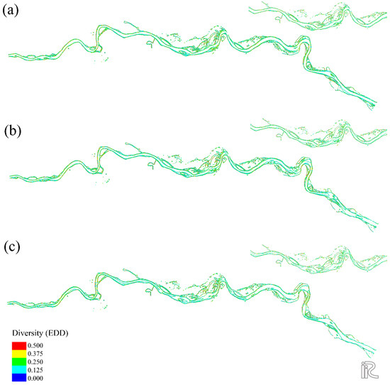
Figure 4.
Simulated Eco-Environmental Diversity index for the (a) maximum, (b) mean and (c) minimum discharge.
Given the relatively large spatial scale adopted to discretize the domain and the low variability of the EDD index along the reach, even if relatively extreme events are considered, its averaged value over the whole reach can be assumed as a good proxy for describing the overall river behaviour (Figure 5).
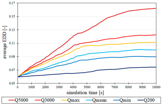
Figure 5.
Averaged Eco-Environmental Diversity index along the reach.
Looking at the very long term of flow discharges measured along the Po River [45], one can notice a slight decrease in recent years, which could be explained by the combined effect of increased human pressure and climate change. While the maximum values are fairly constant in the long term, a decrease is observable in the minima, with more prolonged droughts during the summer months.
As recognizable in Figure 5, this decline in the flow discharge involves a decrease in the habitat conditions, here represented by the averaged EDD index, potentially threatening the overall river biota. Indeed, for very low discharges that last for long periods, no increase of the EDD index is observable anymore, meaning that no fish species can increase in number.
5. Discussion
The opportunity to combine two different solvers permits us to provide some insights about the possible changes on habitat conditions because of an alteration of the present river regime, which is paramount to driving future management. Indeed, since such alterations are related to both natural (climate change) and anthropogenic (dams, diversions) stressors, with different consequences on the fish community, they have to be adequately quantified for designing adaptation strategies at the regional and local scales. In this sense, the actual knowledge does not permit a reliable quantification of the impact of these external drivers on ecosystem services and habitat conditions [47,48]. In fact, there are many shortcomings related to data availability and numerical coding that prevent the application of cascading modelling tools to gain reliable estimates. On the other hand, a lack of knowledge about water‒sediment‒biota interactions, especially in high anthropized environments, is a major challenge for scientists interested in adequately schematizing and reproducing these processes [49].
Regarding the preliminary outcomes reported in this paper, the use of two combined modelling tools provides qualitative indications of the response of the river habitat to different hydrological drivers, but the limitations of the codes clearly affect the final results. Even if the hydrodynamics are reproduced in quite a reliable manner with respect to the measured ones [44], there are many shortcomings that should be highlighted. On the one hand, as previously pointed out, a lack of consideration of the sediment transport and the fluvial morphodynamics can involve an underestimation of the habitat changes, especially in sandy-bedded rivers like the Po. Indeed, with the bed geometry being constant, the water depth is directly correlated to the flow discharge, and therefore fixed in time. However, it is well known that, because of stream morphodynamics, flow hydraulics and aquatic habitat are closely linked and sensitive to changes in the governing conditions [50,51], and any alteration in the natural variability of the flow conditions can potentially result in changes in both the local hydro-morphology and the fluvial habitat. Generally, in fact, both high and low flow conditions affect the aquatic habitat, with a different magnitude depending on the geomorphic structure of the riverbed (i.e., gravel or sand) and its channel forms (i.e., braided, single-thread, meandering, etc.) [52,53], the river hydrology [54,55] and the habitat resilience. On the other hand, the outcomes reported here should be considered only as a qualitative indication of the possible trends of the EDD index, provided that the parameters used for computing it were not calibrated against field evidence because of their lack.
In detail, regarding the habitat parameters assumed for describing the fish preferences in terms of flow depth and velocity, these values derive from a single study performed on the same basin [15] and some default values derived from Japanese streams. Obviously, a better estimate can be performed only using, as a basis, specific information about the fish species present along the reach. An extensive campaign, on the other hand, requires a lot of effort both economically and in terms of workforce, as demonstrated by the lack of field data. Therefore, it is very difficult to get detailed information about the fish population, especially for performing local-scale evaluations in large rivers. The present research represents not only the first application of a modelling technique to qualitatively estimate the changes in the fluvial habitat, but also a tool for pinpoint the need for additional research on fish population, crucial to future hydro-ecological studies.
This first application to a reach of the Po River, however, even if based on several simplifications, pointed out the potential for using numerical modelling as a support tool for river habitat studies. As shown here, there are many shortcomings that should be addressed to build a more reliable model for helping water managers. The steps planned for the future include: (i) the description of the domain by means of a finer grid, aiming to evaluate the very local hydrodynamics instead of the ones at the reach scale, and thus the habitat conditions at a smaller scale; (ii) the use of numerical codes able to reproduce the real hydro-morphodynamics, aiming to include the effect of sediments and solid transport on the fluvial habitat and not only the water-related impact; (iii) the consideration of riparian vegetation along the banks and on bars and islands, with possible effects on the local bed roughness. As for this last parameter, it can be changed spatially, but this requires very detailed spatially distributed information about the water depth, which was not available in this study, to accurately calibrate the 2D code over the whole reach.
Even if the present example shows the potential of the iRIC suite in modelling the fluvial eco-hydrology, several shortcomings are also involved in applying this software. Among others, since the code is still under development, it is not user-friendly like other, more adopted, modelling tools. In particular, the post-processing of the DHABSIM solver is quite simple, and does not provide the user with tabular outcomes, which could eventually be used for elaborating ad hoc metrics for comparing the simulated scenarios. In addition, only a few parameters can be inspected, preventing the opportunity to perform a thorough sensitivity analysis.
Although among the scientific community the topic is still under discussion [56], there is a general agreement that, in the future, the global hydrological cycle will intensify, and extremes of droughts and floods will become more common, fostered by the combined effect of climate change and human pressure. In this context, many Mediterranean and Alpine rivers that used to be permanent tend to become more intermittent, with prolonged droughts, especially during the summer period. As pointed out in similar studies performed on benthic invertebrates [57], although some researchers have claimed that periodic droughts may be important for maintaining the diversity of freshwater systems [58], such shifts highly disturb the environment, with detrimental effects at multiple scales. Even if only from a qualitative point of view, the present study confirms these outcomes, showing that an extremely low discharge can negatively affect the EDD index at the reach scale.
Being a simple schematization of the real world, the modelling cascade proposed here considers just a few variables that can affect the local river habitat. For example, land use practices and climate change are not accounted for in the present application, but they could be very important, especially in highly anthropized environments, even if acting at different spatiotemporal scales. In addition, coupling several models is data- and labour-intensive, and the transferability of the obtained results, especially biological ones, is limited to watercourses and catchments having comparable characteristics [53] and located in similar climatic areas.
Given the need for improving knowledge on hydroecological interactions, the coupling of hydrodynamics and ecological models can be a powerful tool for future research, aiming to evaluate the effect of climate change on the local environment. In the past fluvial hydro-morphology and ecology/biology were generally studied as uncoupled phenomena, with scientists having different backgrounds and using manifold metrics. However, as recently pointed out and also highlighted by this simple example, river environments should be considered as a unicum [59], and studied and modelled as a whole to adequately characterize the interactions between the hydro-morpho-biodynamic processes involved.
On the one hand, the use of numerical codes should always be coupled with a detailed field campaign, aiming to obtain reliable and up-to-date input parameters for calibrating and validating the adopted modelling tool. On the other hand, water managers, practitioners and scientists should work together, aiming to choose the correct numerical model, populate it with the most accurate and field-based data, and derive the main conclusions to better manage the fluvial environment. Only a constant and timely revision of all the adopted numerical tools and monitoring techniques can assure reliable estimates of the future trends of highly anthropized alluvial watercourses, and allow one to plan adequate responses.
6. Conclusions
Using a 70-km reach of the Po River, in Italy, two numerical solvers were combined to first resolve the 2D fluvial hydrodynamics with grids having an area of around 250 m2, and then, based on that, provide a qualitative estimate of the Eco-Environmental Diversity index along the stream. Aiming to characterize the river’s response to different flow discharges, several runs were performed, assuming, as input, constant water flows spanning from flooding to drought conditions, following the long-term hydrology measured along the reach.
Even if based on several simplifications under a modelling point of view and because of the lack of information about the local biota, the preliminary results reported here show, from a qualitative point of view, the dependence of the river habitat on the local hydrology, pointing out the need to improve our knowledge of eco-hydrological processes. Excessive water flow velocity and depth, correlated to flooding events, involves unsustainable conditions for the local fauna, preventing fish spawning and growth because of the high flow velocity. Meanwhile, a prolonged drought state like that recently observed along the Po River affects the community in a similar manner, decreasing the EDD index with detrimental effects on fish.
Thanks to its simplicity, the proposed methodology can be applied for a first, qualitative estimate of the local habitat as a response of changing hydrology, assuming the literature parameters for the biota to overcome the lack of information. However, for providing reliable and quantifiable values, proper calibration and validation of the models should be performed, in particular regarding the biological aspects but also the 2D distribution of the water flow. Based on these promising outcomes and for overcoming the modelling limitations highlighted in the present case study, in the future several improvements are planned, both to the numerical schematization and to the field-based evidence.
Funding
This work was developed within the statutory activities No. 3841/E-41/S/2018 of the Ministry of Science and Higher Education of Poland.
Acknowledgments
Thanks go to the colleagues involved in the INFRASAFE project (infrasafe-project.com), who contributed by developing some ideas reported here and providing some of the data. I thank the three reviewers who contributed to improving the quality of this article through their timely and useful comments.
Conflicts of Interest
The author declares no conflict of interest.
References
- Clemens, S.L. Life on the Mississippi; J. R. Osgood: Boston, MA, USA, 1884. [Google Scholar]
- DeBoer, J.A.; Thoms, M.C.; Casper, A.F.; Delong, M.D. The Response of Fish Diversity in a Highly Modified Large River System to Multiple Anthropogenic Stressors. J. Geophys. Res. Biogeosci. 2019. [Google Scholar] [CrossRef]
- Lake, P.S. Disturbance, patchiness, and diversity in streams. J. N. Am. Benthol. Soc. 2000, 19, 573–592. [Google Scholar] [CrossRef]
- Leigh, C.; Sheldon, F.; Kingsford, R.T.; Arthington, A.H. Sequential floods drive ‘booms’ and wetland persistence in dryland rivers: A synthesis. Mar. Freshw. Res. 2010, 61, 896–908. [Google Scholar] [CrossRef]
- Foerst, M.; Rüther, N. Bank Retreat and Streambank Morphology of a Meandering River during Summer and Single Flood Events in Northern Norway. Hydrology 2018, 5, 68. [Google Scholar] [CrossRef]
- Ormerod, S.J.; Dobson, M.; Hildrew, A.G.; Townsend, C. Multiple stressors in freshwater ecosystems. Freshw. Biol. 2010, 55, 1–4. [Google Scholar] [CrossRef]
- Tockner, K.; Stanford, J.A. Riverine flood plains: Present state and future trends. Environ. Conserv. 2002, 29, 308–330. [Google Scholar] [CrossRef]
- Nilsson, C.; Jansson, R.; Malmqvist, B.; Naiman, R.J. Restoring riverine landscapes: The challenge of identifying priorities, reference states, and techniques. Ecol. Soc. 2007, 12, 16. [Google Scholar] [CrossRef]
- Lanzoni, S.; Luchi, R.; Bolla Pittaluga, M. Modeling the morphodynamic equilibrium of an intermediate reach of the Po River (Italy). Adv. Water Resour. 2015, 81, 92–102. [Google Scholar] [CrossRef]
- Nones, M.; Ronco, P.; Di Silvio, G. Modelling the impact of large impoundments on the Lower Zambezi River. Int. J. River Basin Manag. 2013, 11, 221–236. [Google Scholar] [CrossRef]
- Schleiss, A.J.; Franca, M.J.; Juez, C.; De Cesare, G. Reservoir sedimentation. J. Hydraul. Res. 2016, 54, 595–614. [Google Scholar] [CrossRef]
- Strayer, D.L. Alien species in fresh waters: Ecological effects, interactions with other stressors, and prospects for the future. Freshw. Biol. 2010, 55, 152–174. [Google Scholar] [CrossRef]
- Bosa, S.; Petti, M.; Pascolo, S. Numerical Modelling of Cohesive Bank Migration. Water 2018, 10, 961. [Google Scholar] [CrossRef]
- Esmaeili, T.; Sumi, T.; Kantoush, S.A.; Kubota, Y.; Haun, S.; Rüther, N. Three-Dimensional Numerical Study of Free-Flow Sediment Flushing to Increase the Flushing Efficiency: A Case-Study Reservoir in Japan. Water 2017, 9, 900. [Google Scholar] [CrossRef]
- Gavioli, A.; Mancini, M.; Milardi, M.; Aschonitis, V.; Racchetti, E.; Viaroli, P.; Castaldelli, G. Exotic species, rather than low flow, negatively affect native fish in the Oglio River, Northern Italy. River Res. Appl. 2018, 34, 887–897. [Google Scholar] [CrossRef]
- Nones, M.; Varrani, A. Sensitivity Analysis of a Riparian Vegetation Growth Model. Environments 2016, 3, 30. [Google Scholar] [CrossRef]
- Thoms, M.C.; Meitzen, K.M.; Julian, J.P.; Butler, D.R. Bio-geomorphology and resilience thinking: Common ground and challenges. Geomorphology 2018, 305, 1–7. [Google Scholar] [CrossRef]
- Juez, C.; Bühlmann, I.; Maechler, G.; Schleiss, A.J.; Franca, M.J. Transport of suspended sediments under the influence of bank macro-roughness. Earth Surf. Process. Landf. 2018, 43, 271–284. [Google Scholar] [CrossRef]
- Nelson, J.M.; Shimizu, Y.; Abe, T.; Asahi, K.; Gamou, M.; Inoue, T.; Iwasaki, T.; Kakinuma, T.; Kawamura, S.; Kimura, I.; et al. The international river interface cooperative: Public domain flow and morphodynamics software for education and applications. Adv. Water Resour. 2016, 93, 62–74. [Google Scholar] [CrossRef]
- Vezzoli, R.; Mercogliano, P.; Pecora, S.; Zollo, A.L.; Cacciamani, C. Hydrological simulation of Po River (North Italy) discharge under climate change scenarios using the RCM COSMO-CLM. Sci. Total Environ. 2015, 521, 346–358. [Google Scholar] [CrossRef] [PubMed]
- Simpson, E.H. Measurement of diversity. Nature 1949, 163, 688. [Google Scholar] [CrossRef]
- iRIC Software. DHABSIM Solver Manual. 2017. Available online: https://i-ric.org/en/solvers/dhabsim/ (accessed on 25 November 2018).
- Kozarek, J.L.; Hession, W.C.; Dolloff, C.A.; Diplas, P. Hydraulic Complexity Metrics for Evaluating In-Stream Brook Trout Habitat. J. Hydraul. Eng. 2010, 136, 1067–1076. [Google Scholar] [CrossRef]
- Maselli, V.; Pellegrini, C.; Del Bianco, F.; Mercorella, A.; Nones, M.; Crose, L.; Guerrero, M.; Nittrouer, J.A. River Morphodynamic Evolution Under Dam-Induced Backwater: An Example from the Po River (Italy). J. Sediment. Res. 2018, 88, 1190–1204. [Google Scholar] [CrossRef]
- Domeneghetti, A.; Carisi, F.; Castellarin, A.; Brath, A. Evolution of flood risk over large areas: Quantitative assessment for the Po River. J. Hydrol. 2015, 527, 809–823. [Google Scholar] [CrossRef]
- Montanari, A. Hydrology of the Po River: Looking for changing patterns in river discharge. Hydrol. Earth Syst. Sci. 2012, 16, 3739–3747. [Google Scholar] [CrossRef]
- Cozzi, S.; Giani, M. River water and nutrient discharge in the Northern Adriatic Sea: Cur-rent importance and long term changes. Cont. Shelf Res. 2011, 31, 1881–1893. [Google Scholar] [CrossRef]
- Syvitski, J.P.M.; Kettner, A.J. On the flux of water and sediment into the Northern Adriatic Sea. Cont. Shelf Res. 2007, 27, 296–308. [Google Scholar] [CrossRef]
- Lamberti, A.; Schippa, L. Studio dell’abbassamento del fiume Po: Previsioni trentennali di abbassamento a Cremona. In Supplemento a Navigazione Interna, Rassegna Trimestrale di Studi e Informazioni; Azienda Regionale per i Porti di Cremona e Mantova: Cremona, Italy, 1994. (In Italian) [Google Scholar]
- Guerrero, M.; Di Federico, V.; Lamberti, A. Calibration of a 2-D morphodynamic model using water-sediment flux maps derived from an ADCP recording. J. Hydroinform. 2013, 15, 813–828. [Google Scholar] [CrossRef]
- Juez, C.; Battisacco, E.; Schleiss, A.J.; Franca, M.J. Assessment of the performance of numerical modeling in reproducing a replenishment of sediments in a water-worked channel. Adv. Water Resour. 2016, 92, 10–22. [Google Scholar] [CrossRef]
- Bovee, K.D. A guide to stream habitat analysis using the instream incremental methodology. In Instream Flow Paper; Fish and Wildlife Services, U.S. Dept. of Interior: Washington, DC, USA, 1982. [Google Scholar]
- Booker, D.J.; Dunbar, M.J. Application of physical habitat simulation (PHABSIM) modelling to modified urban river channels. River Res. Appl. 2004, 20, 167–183. [Google Scholar] [CrossRef]
- Clark, J.S.; Rizzo, D.M.; Watzin, M.C.; Hession, W.C. Spatial distribution and geomorphic condition of fish habitat in streams: An analysis using hydraulic modeling and geostatistics. River Res. Appl. 2008, 24, 885–889. [Google Scholar] [CrossRef]
- Shen, Y.; Diplas, P. Application of two- and three dimensional computational fluid dynamics models to complex ecological stream flows. J. Hydrol. 2008, 348, 195–214. [Google Scholar] [CrossRef]
- Nones, M.; Pugliese, A.; Domeneghetti, A.; Guerrero, M. Po River morphodynamics modelled with the open-source code iRIC. In Free Surface Flows and Transport Processes. GeoPlanet: Earth and Planetary Sciences; Kalinowska, M., Mrokowska, M., Rowiński, P., Eds.; Springer: Cham, Switzerland, 2018. [Google Scholar]
- Ghanem, A.H.; Steffler, P.M.; Hicks, F.E.; Katopodis, C. Two-dimensional hydraulic simulation of physical habitat conditions in flowing streams. River Res. Appl. 1996, 12, 185–200. [Google Scholar] [CrossRef]
- Steffler, P.; Blackburn, J. River2D: Two-Dimensional Depth Averaged Model of River Hydrodynamics and Fish Habitat. In Introduction to Depth Averaged Modeling and User’s Manual; University of Alberta: Edmonton, AB, Canada, 2002; Available online: http://www.river2d.ualberta.ca/Downloads/documentation/River2D.pdf (accessed on 30 November 2018).
- iRIC Software. River2D Tutorials. 2016. Available online: https://i-ric.org/en/solvers/river2d/ (accessed on 10 July 2018).
- Hicks, F.E.; Steffler, P.M. Characteristic Dissipative Galerkin Scheme for Open-Channel Flow. J. Hydraul. Eng. 1992, 118, 337–352. [Google Scholar] [CrossRef]
- Gard, M. Comparison of spawning habitat predictions of PHABSIM and River2D models. Int. J. River Basin Manag. 2009, 7, 55–71. [Google Scholar] [CrossRef]
- Canning, A.D.; Death, R.G. Ecosystem Health Indicators-Freshwater Environments. In Encyclopedia of Ecology; Elsevier: Amsterdam, The Netherlands, 2019. [Google Scholar]
- Minns, C.K. Allometry of home range size in lake and river fishes. Can. J. Fish. Aquat. Sci. 1995, 52, 1499–1508. [Google Scholar] [CrossRef]
- Nones, M.; Guerrero, M.; Conevski, S.; Ruther, N.; Di Federico, V. The acoustic backscatter at two well-spaced grazing angles to characterize moving sediments at riverbed. In Proceedings of the XXXVI Convegno Nazionale di Idraulica e Costruzioni Idrauliche, Ancona, Italy, 12–14 September 2018. [Google Scholar]
- Zanchettin, D.; Traverso, P.; Tomasino, M. Po River discharges: A preliminary analysis of a 200-year time series. Clim. Chang. 2008, 89, 411–433. [Google Scholar] [CrossRef]
- Nones, M.; Archetti, R.; Guerrero, M. Time-Lapse Photography of the Edge-of-Water Line Displacements of a Sandbar as a Proxy of Riverine Morphodynamics. Water 2018, 10, 617. [Google Scholar] [CrossRef]
- Datry, T.; Boulton, A.J.; Bonada, N.; Fritz, K.; Leigh, C.; Sauquet, E.; Tockner, K.; Hugueny, B.; Dahm, C.N. Flow intermittence and ecosystem services in rivers of the Anthropocene. J. Appl. Ecol. 2018, 55, 353–364. [Google Scholar] [CrossRef] [PubMed]
- Herrera Pérez, J.; Parra, J.L.; Restrepo-Santamaría, D.; Jiménez-Segura, L.F. The Influence of Abiotic Environment and Connectivity on the Distribution of Diversity in an Andean Fish Fluvial Network. Front. Environ. Sci. 2019, 7, 9. [Google Scholar] [CrossRef]
- Radinger, J.; Wolter, C.; Kail, J. Spatial scaling of environmental variables improves species-habitat models of fishes in a small, sand-bed lowland river. PLoS ONE 2015, 10, e0142813. [Google Scholar] [CrossRef] [PubMed]
- Tamminga, A.; Eaton, B. Linking geomorphic change due to floods to spatial hydraulic habitat dynamics. Ecohydrology 2018, 11, e2018. [Google Scholar] [CrossRef]
- Nagata, T.; Watanabe, Y.; Yasuda, H.; Ito, A. Development of a meandering channel caused by the planform shape of the river bank. Earth Surf. Dyn. 2014, 2, 255–270. [Google Scholar] [CrossRef]
- Gostner, W.; Alp, M.; Schleiss, A.J.; Robinson, C.T. The hydro-morphological index of diversity: A tool for describing habitat heterogeneity in river engineering projects. Hydrobiologia 2013, 712, 43–60. [Google Scholar] [CrossRef]
- Sukhodolov, A.; Bertoldi, W.; Wolter, C.; Surian, N.; Tubino, M. Implications of channel processes for juvenile fish habitats in Alpine rivers. Aquat. Sci. 2009, 71, 338. [Google Scholar] [CrossRef]
- Elosegi, A.; Díez, J.; Mutz, M. Effects of hydromorphological integrity on biodiversity and functioning of river ecosystems. Hydrobiologia 2010, 657, 199–215. [Google Scholar] [CrossRef]
- Guse, B.; Kail, J.; Radinger, J.; Schröder, M.; Kiesel, J.; Hering, D.; Wolter, C.; Fohrer, N. Eco-hydrologic model cascades: Simulating land use and climate change impacts on hydrology, hydraulics and habitats for fish and macroinvertebrates. Sci. Total Environ. 2015, 533, 542–556. [Google Scholar] [CrossRef] [PubMed]
- Hisdal, H.; Stahl, K.; Tallaksen, L.M.; Demuth, S. Have streamflow droughts in Europe become more severe or frequent? Int. J. Climatol. 2001, 21, 317–333. [Google Scholar] [CrossRef]
- Fenoglio, S.; Bo, T.; Cucco, M.; Malacarne, G. Response of benthic invertebrate assemblages to varying drought conditions in the Po river (NW Italy). Ital. J. Zool. 2007, 74, 191–201. [Google Scholar] [CrossRef]
- Everard, M. The benefits of drought to the aquatic environment. Freshw. Forum 1996, 7, 33–50. [Google Scholar]
- Vesipa, R.; Camporeale, C.; Ridolfi, L. Effect of river flow fluctuations on riparian vegetation dynamics: Processes and models. Adv. Water Resour. 2017, 110, 29–50. [Google Scholar] [CrossRef]
© 2019 by the author. Licensee MDPI, Basel, Switzerland. This article is an open access article distributed under the terms and conditions of the Creative Commons Attribution (CC BY) license (http://creativecommons.org/licenses/by/4.0/).