Effect of the Concentration of Sand in a Mixture of Water and Sand Flowing through PP and PVC Elbows on the Minor Head Loss Coefficient

Abstract

The article presents the results of tests of minor head losses through PVC and PP elbows for a flow of water and mixtures of water and sand with grain sizes of up to 0.5 mm and concentrations of 5.6 g·L⁻¹, 10.84 g·L⁻¹, and 15.73 g·L⁻¹. The tests were carried out at variable flow velocities for three elbow diameters of 63 mm, 75 mm, and 90 mm. The flow rate, pressure difference in the tested cross-sections, and temperature of the fluids were measured and automatically recorded. The results of the measurements were used to develop mathematical models for determining the minor head loss coefficient as a function of elbow diameter, sand concentration in the liquid, and Reynolds number. The mathematical model was developed by cross validation. It was shown that when the concentration of sand in the liquid was increased by 1.0 g∙L⁻¹, the coefficient of minor head loss through the elbows increased, in the Reynolds number range of 4.6 × 10⁴–2.1 × 10⁵, by 0.3–0.01% for PP63, 0.6–0.03% for PP75, 1.1–0.06% for PP90, 0.8−0.01% for PVC63, 0.8–0.02% for PVC75, and 0.9–0.04% for PVC90. An increase in Re from 5 × 10⁴ to 2 × 10⁶ for elbows with diameters of 63, 75 and 90 mm caused a 7.3%, 6.8%, and 6.0% decrease in the minor head loss coefficient, respectively.

1. Introduction

Easy and quick determination of head losses through fittings in a piping system is particularly important, because it allows us to select pumps for proper operation of the system. The essential components of a piping system are elbows. This is because as a rule, pipes in a system are connected by many elbows and these fittings strongly affect the overall head losses of the entire system. The total pressure difference between the inlet and outlet of a fitting is given by Formula (1) [1,2].

$$p_{in}-p_{out}=\zeta \cdot \frac{\rho \cdot v^2}{2}$$

(1)

where: v—mean flow velocity upstream of the fitting, m·s⁻¹, ζ—dimensionless coefficient of minor head loss, ρ—fluid density, kg·m⁻³.

Often, Formula (1) is divided by ρ·g to transform it into another formula which gives the difference in pressure height in meters. Then, it has the form (2), where g is the acceleration of gravity in m·s⁻².

$$h=\zeta \cdot \frac{v^2}{2\cdot g}$$

(2)

Investigations of the behavior of liquids flowing through elbows show that this flow involves very complex phenomena, with many factors affecting head loss. According to some authors, a key factor is the curvature ratio, which is r/D = 1.0 for so-called short-radius elbows [3,4], and r/D = 1.5 for long-radius elbows [3,5]. These researchers have shown that in short-radius elbows with an r/D = 1, centrifugal force leads to the formation of a separated region on the inner wall side, in which counter-rotating flow cells known as Dean vortices are induced [6], in long-radius elbows, this area is smaller and is formed intermittently [3]. In these regions, flow is very dynamic, and the presence of sand particles may lead to erosion caused by the grains hitting against elbow walls. Duarte et al. [7] found that sand-induced erosion was most severe in the region between 40° to 60° from the inlet, where angle 0° is the inlet to the elbow and 90° is the outlet. They also found that the depth of erosion decreased with increasing surface roughness. The addition of air bubbles to water significantly intensifies the erosive action of sand [8]. Especially important is the amount of air and its flow rate. Air affects the erosion rates of elbow walls much more strongly than water. Viejra et al. [8] demonstrated, for vertical upward flow, that at a water flow rate of 0.04 m·s⁻¹ and air velocity of 15–27 m·s⁻¹, the erosion rate resulting from the injection of sand into the gas stream was 3.3–9.26 × 10⁻⁴ mm·kg⁻¹ sand. For flows of mixtures of water and air, pressure losses are affected not only by the flow velocities of both of these factors, but also by whether the flow is vertical, horizontal, or diagonal [8,9]. In the case of vertical pipelines, coalescence leads to the formation of gas voids in the elbow which reduce the cross-sectional area of liquid flow [10,11]. Air-water flow leads to a strong dissipation of the gas; the strongest dissipation was obtained between 3D and 9D upstream of an elbow (D—pipe diameter) [11]. Dissipation was found to be a linear function of Reynolds number [12].

Dynamic changes in fluid behavior during flow through an elbow were computationally modeled by reference [13], who showed that high pressure gradients formed on the inner surfaces of the elbows causing pulsed acceleration and deceleration of the flow, which led to strong turbulence and difficult-to-estimate secondary head losses [14]. Turbulence can be limited by wedge-shaped inserts, which, according to reference [15], may not be larger than one fourth of the diameter of the pipe connected to the elbow. These tests, however, were performed for elbow and T-junction close-coupled pipes, which means that the maximum wedge height could be different for a system without a T-junction (an elbow alone). Of course, the solution with a curvilinear modification of the inner surface of the elbow can be used in an experimental installation, but is much more difficult to deploy in real-life settings, especially in systems with changing flow directions.

More complicated phenomena are observed in pipelines in which elbows are connected by very short pipe sections, i.e., when they are located very close to each other. Such systems are subject to the formation of transverse and longitudinal vortices, and, as shown by reference [16] in an experiment in which the distance between the elbows was only 0.57D (D—pipe diameter), the first elbow generated very strong vortices in the second one, leading to an increase in total head loss. In cases where a larger number of elbows are installed serially, the vortices transfer from one elbow to the next [17]. Shiraishi et al. [1] pointed out, quoting Idelchik, that the local head loss coefficient should be considered separately for different ranges of the Reynolds number. In the subcritical range Re < 1 × 10⁵ the values of coefficient ζ are unstable, while in the transitional range 1 × 10⁵ < Re < 4 × 10⁵, the value of ζ drops from around 2.3 to 1.38 along with increasing Re. In the post-critical range Re > 4 × 10⁵, coefficient ζ has a constant value of 1.38, regardless of changes in Re. Ma and Zhang [2] obtained ζ = 1.1 for an elbow during water flow; this value was constant for the flow velocity range of 0.5–2.4 m·s⁻¹ and Reynolds number > 6900.

Numerical values of coefficient ζ for specific fittings and valves are determined in tests [18] and depend primarily on the geometrical shape and diameter of the fitting, roughness of its inner wall, the way the fitting is secured to the pipe, etc. [19,20,21].

In storm drainage systems, runoff water always contains sand, which is rinsed from the ground surface to storm drains and further down into the network. Pumping such a mixture through the system requires the use of a suitable pump, which must be selected on the basis of major and minor head loss data [22]. The influence of sand on head losses has been confirmed in studies which show that head losses increase with increasing sand concentration and grain size [23]. The drop in pressure is smaller when water with sand flows vertically than when it flows horizontally, all other things being equal [24]. For high concentrations of suspended solids, when the fluid flowing through the pipeline diverges from Newton’s models, other types of analyses are used [25,26].

Not all results reported in the literature can be applied in practice. A substantial number of studies analyze a particular phenomenon in non-commercial elbows of pre-defined shapes and sizes made especially for experimental purposes from special (e.g., transparent) materials [4,5,7]. Of course, this allows researchers to demonstrate the occurrence of and explain the essence of certain physical phenomena, but the results obtained in this way are not always suitable for use in engineering practice. Practicable results can be obtained by analyzing the hydraulic parameters of commercial elbows commonly used in storm drainage systems.

The aim of the research was to determine by experiment method the influence of sand concentration in water transported by pipeline on the local head loss coefficient for PP and PVC elbows. The independent variables were: the type and diameter of the elbows, the flow rate of the liquid, the concentration of sand. There are no models in the literature that take into account the effect of sand concentration and Reynolds number on the level of local losses. This article attempts to develop such a model for PP and PVC elbows.

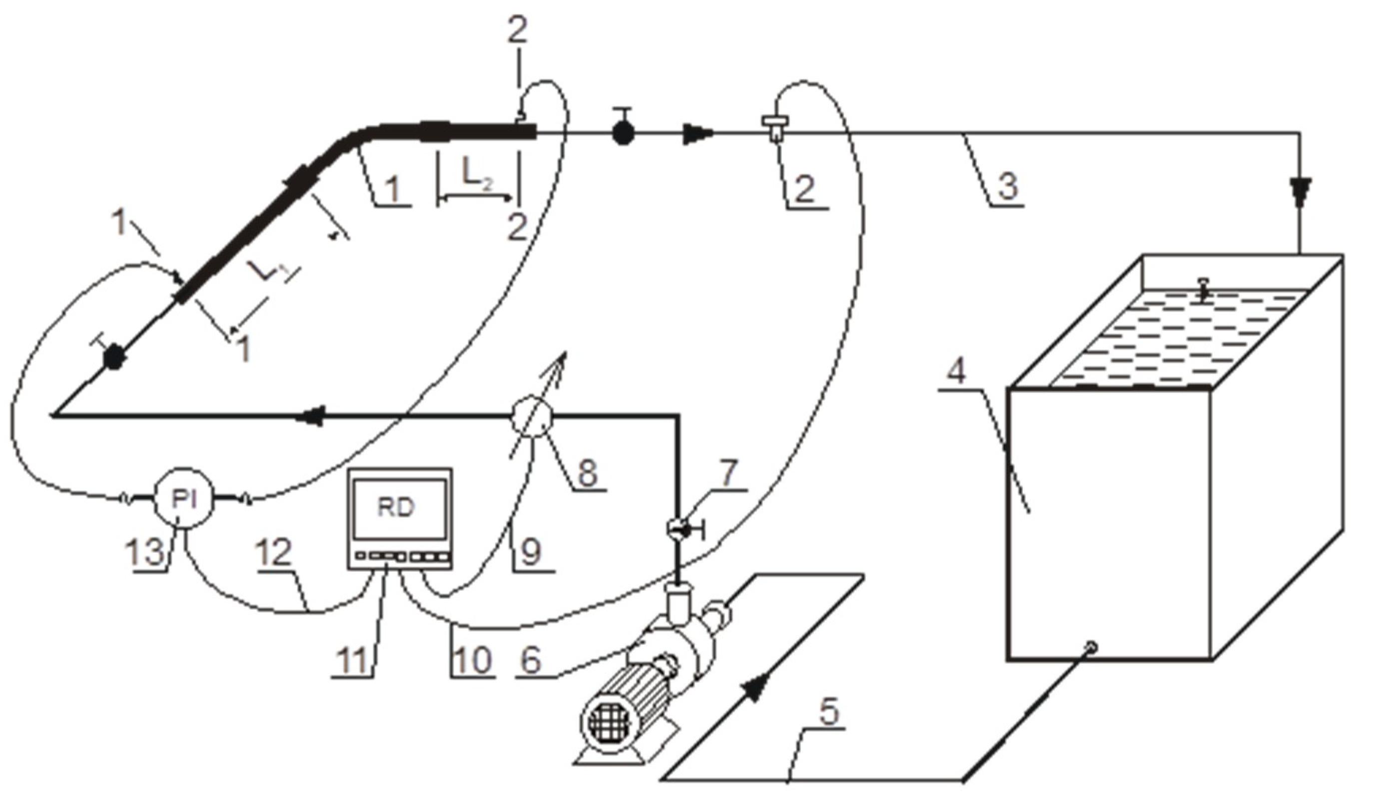
2. Materials and Methods

The tests were carried out at variable flow velocities for three elbow diameters of 63, 75, and 90 mm on the test stand shown in Figure 1. The test elbow (1) was connected to a loop-shaped pipeline. The liquid was drawn from a tank (4) and pumped by pump (6) through the loop of pipes back to the tank. Flow rates were measured with a PROMAG 53 flow meter (8), hydraulic losses were determined using a DELTABAR S differential pressure gauge (13), and the temperature of the liquid was measured using a TMR31 thermometer (2). Due to the sensitivity of the devices and the fast-changing readings resulting from the pulsation of the flux, the readings were recorded at 1 s time intervals using an RSG40 memograph (11). All measuring devices had been purchased from Endress+Hauser (Reinach, Switzerland). Changes in the flow rate were determined using a needle valve (7).

As the literature shows [21,27,28], key to the reliability of measurements is the way elbows are connected to adjacent pipes. An improper joint, whether welded, bonded, threaded or other, can generate additional head losses of unknown value. It is particularly important that identical joints be used when elbows made of different materials and with different diameters are tested.

Analyzing the problem of minor head loss coefficient ζ, one should also take into account hydraulic resistance related to the connection of the fitting with the straight line sections of the pipelines. In fact, connections and straight sections connecting the fitting also generate hydraulic resistance. Current literature often lacks information on whether the determined minor head loss coefficient ζ applies to fittings (elbows, valves etc.) themselves, or also applies to the resistance generated on the connections and rectilinear sections of pipelines connecting the fittings [26,29,30,31]. According to the methodology for determining the minor head loss coefficients given in the standard from reference [32], hydraulic resistance generated on the connections and straight sections of pipelines connecting the fitting should be taken into account. Therefore, hydraulic resistance that arises at the connections and straight sections of the pipelines connecting the fitting should not be calculated, but instead should be measured. The accuracy of the calculations of hydraulic resistances generated on joints and straight sections of pipelines connecting the fitting will depend on the value of coefficient of linear resistance λ adopted and calculated and assumed coefficient of roughness absolute k. In this measuring stand, hydraulic resistance on connections and straight sections of pipelines joining the elbow were measured and taken into account in the determination of minor head loss coefficients ζ in the tested elbows made of PP and PVC.

In the test stand used in the present study, all fittings were connected to pipes by identical joints, both with regard to their method of assembly and the length of reducer pipes. The PP elbows were screwed in place using a threaded connection with an O-ring rubber seal and a lip seal. PVC elbows were adhesive bonded. The inlet/outlet openings and impulse piping were located at L₁ = 5D downstream of the fitting and at L₂ = 3D upstream of the fitting, as recommended by Endress+Hauser in their installation manual for DELTABAR S differential pressure gauge, in which the manufacturer refers users to DIN 19210 recommendations for routing pressure piping. Analogously, for the flow meter (PROMAG), inlet and outlet runs were maintained to attain the specified level of accuracy of the measuring device. The tests were carried out using 63 × 3.0, 75 × 3.6 and 90 × 4.3 PN 10 PVC pipes.

The tests were carried out in four series using water and water mixed with river sand with a grain size <0.5 mm at the following concentrations: C1 = 5.6 g·dm⁻³, C2 = 10.84 g·dm⁻³, and C3 = 15.73 g·dm⁻³. The concentration of sand in the mixtures was determined in accordance with reference [33]. Liquid flow rates were in the range of 5–40 m³·h⁻¹ and were increased in increments of 5 m³·h⁻¹.

Because the test elbows had been installed in a horizontal position and the connecting pipelines had the same diameters, accordance with reference [32], the classic Bernoulli equation for the test cross-sections could be represented by Equation (3)

$$\frac{p_1-p_2}{\rho \cdot g}=h_{str1-2}=\left(\lambda \cdot \frac{l_1}{D}+\zeta +\lambda \cdot \frac{l_2}{D}\right)\cdot \frac{8\cdot Q^2}{{\pi }^2\cdot g\cdot D^4}$$

(3)

where: l₁ and l₂ stand for the inlet/outlet run lengths (distances of test cross-sections from the axis of the fitting), respectively.

After transformations, an equation was obtained which allowed to determine coefficient ζ as a function of flow rate Q or flow velocity V

$$\zeta =\frac{p_1-p_2}{\rho \cdot g}\cdot \frac{{\pi }^2\cdot g\cdot D^4}{8\cdot Q^2}-\left(\lambda \cdot \frac{l_1+l_2}{D}\right)=\frac{p_1-p_2}{\rho \cdot g}\cdot \frac{2\cdot g}{V^2}-\left(\lambda \cdot \frac{l_1+l_2}{D}\right)$$

(4)

Pressure difference p₁ − p₂ and flow rate Q were read from the respective gauges. Major head loss coefficient λ was calculated using the Phama formula [34], where the viscosity of water was determined, using liquid temperature measurements, from a relationship obtained by Polynomial Approximation (5) of points tabulated in a study by reference [35]. The viscosity of water with suspended solids was calculated using the Einstein Formula (6) [36].

$${\nu }_w=t^2\times 6.9\times {10}^{-10}-t\times 5.25\times {10}^{-8}+1.77\times {10}^{-6}$$

(5)

$${\nu }_z={\nu }_w\times \left(1+2.5\times C_z\right)$$

(6)

where: t—liquid temperature, C_z—concentration of suspended solids in kg·m⁻³.

Equation (4) was transformed into (7), a form that was more suitable for modeling ζ = f(Re), where the Reynolds number was number was $\mathrm{Re}=\frac{4\cdot Q}{\pi \cdot d\cdot \nu }$.

$$\zeta =\frac{p_1-p_2}{\rho \cdot g}\cdot \frac{2\cdot g\cdot D^2}{{\mathrm{Re}}^2\cdot {\nu }^2}-\left(\lambda \cdot \frac{l_1+l_2}{D}\right)$$

(7)

3. Results

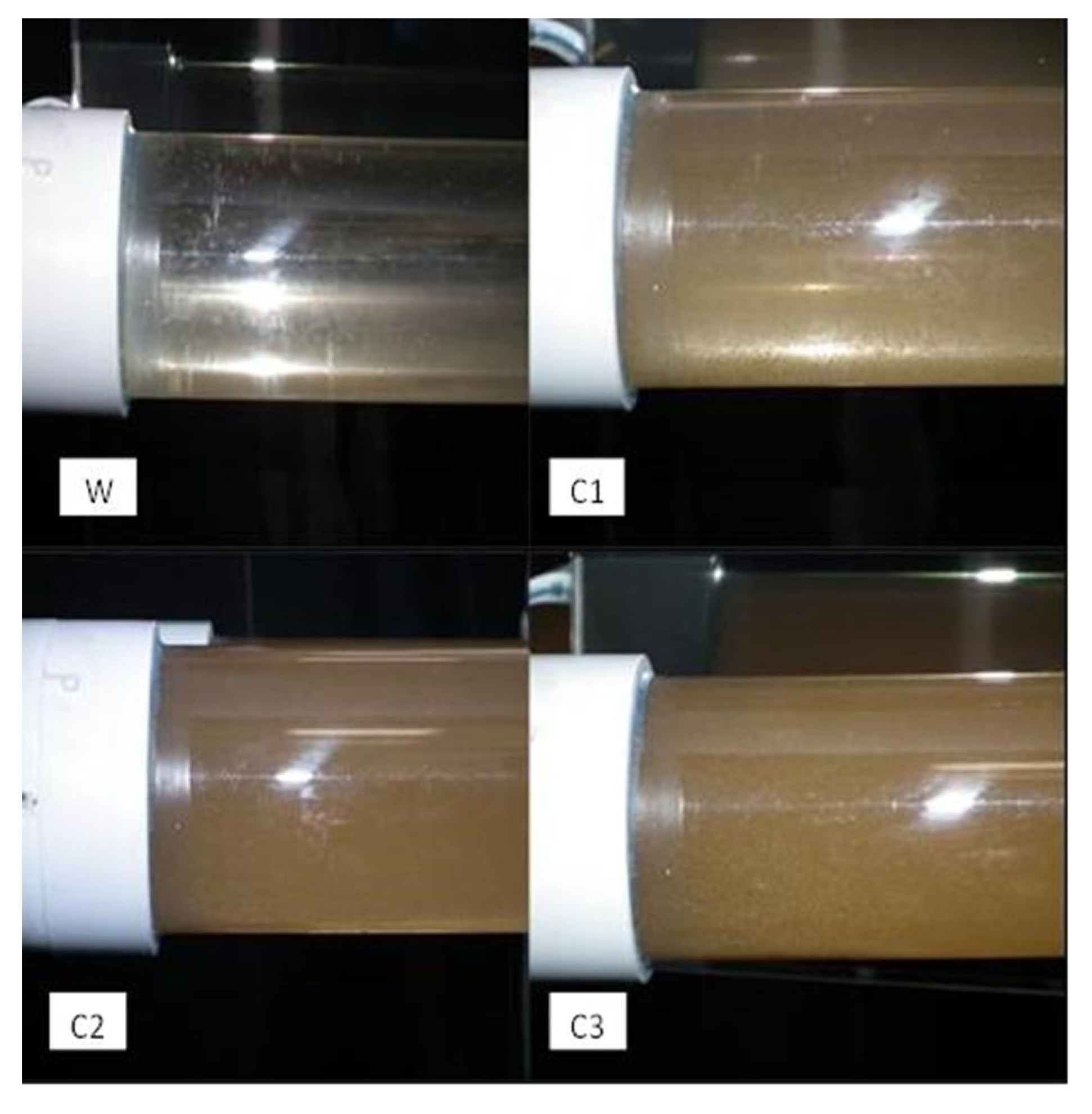
3.1. Hydraulic Conditions of Flow the Mixture Water and Sand

Sand with a maximum particle diameter of 0.5 mm was selected to obtain a liquid with a dispersion value that would prevent sand from being dragged along the bottom of the pipeline. Calculations of sedimentation rate V_s showed that the maximum grain size in the Stokes range (Re < 0.4) was 0.091 mm, and the minimum grain size in the Newton range (Re > 1000) was 3.25 mm. It follows that the particles of sand used in the experiments sedimented at rates described by the Allan model (Equation (8)). This model was used to calculate the settling rate for 0.5 mm-diameter grains, which was 0.062 m·s⁻¹ (Re = 23.8) [36].

$$V_s=0.1528\cdot \frac{{\left({\rho }_s-{\rho }_f\right)}^{0.714}\cdot d^{1.143}\cdot g^{0.714}}{{\rho }_f{}^{0.286}\cdot {\mu }^{0.427}}$$

(8)

where: ρ_s and ρ_f—sand and water densities, d—diameter grains of sand, g—acceleration of the earth and μ—dynamic coefficient of water viscosity.

At the tested sand concentrations, the porosity calculated using the Richardson-Zaki equation was nearly 1, which meant the particles would settle freely through the fluid (free settling). Grains with a maximum diameter of 0.5 mm could sediment at a flow velocity lower than that determined by the simplified Newitt equation Vo = 17V_s = 17 × 0.062 = 1.05 m·s⁻¹ [36,37]. Under the assumed testing conditions, flow velocities for the vast majority of sand particles were higher at 0.78–4.3 m·s⁻¹ for 63 mm elbows, 0.8–3.1 m·s⁻¹ for 75 mm elbows, and 0.8–2.1 m·s⁻¹ for 90 mm elbows. In all series of tests, where the water flow rate was 10 m³·h⁻¹ and the higher limiting grain velocity determined by the Newitt formula was smaller than the actual flow velocities. Therefore, all grains were lifted with water. Only at the intensity of 5 m³·h⁻¹, grains with a diameter of 0.385–0.5 mm could sediment and occupy the lower part of the water layer in PP63 and PVC63 and 0.395–0.5 mm in PP75, PVC75, PP90 and PVC90. It can be said that sand was practically fully dispersed in water, as observed in transparent sections of the installation. Figure 2 shows dispersion of sand in water for the particular sand concentrations C1, C2 and C3 at a flow velocity of about 1 m·s⁻¹. Image W shows clear water.

As shown in the successive images in Figure 2, along with increasing concentrations of sand in water, the mixture becomes distinctly more turbid. None of the pictures show a sand layer deposited at the bottom of the pipe or dragged sand grains. This leads to the conclusion that the particle transport rate is high enough to ensure full dispersion of sand.

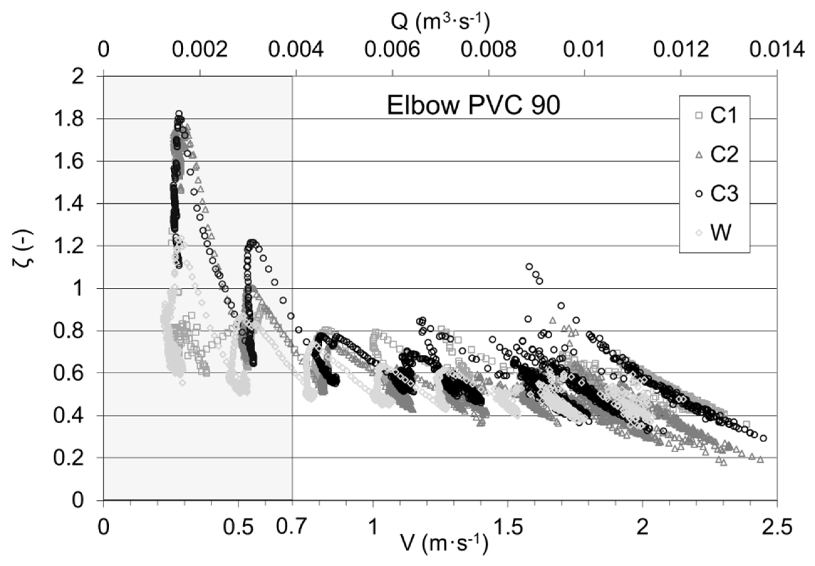
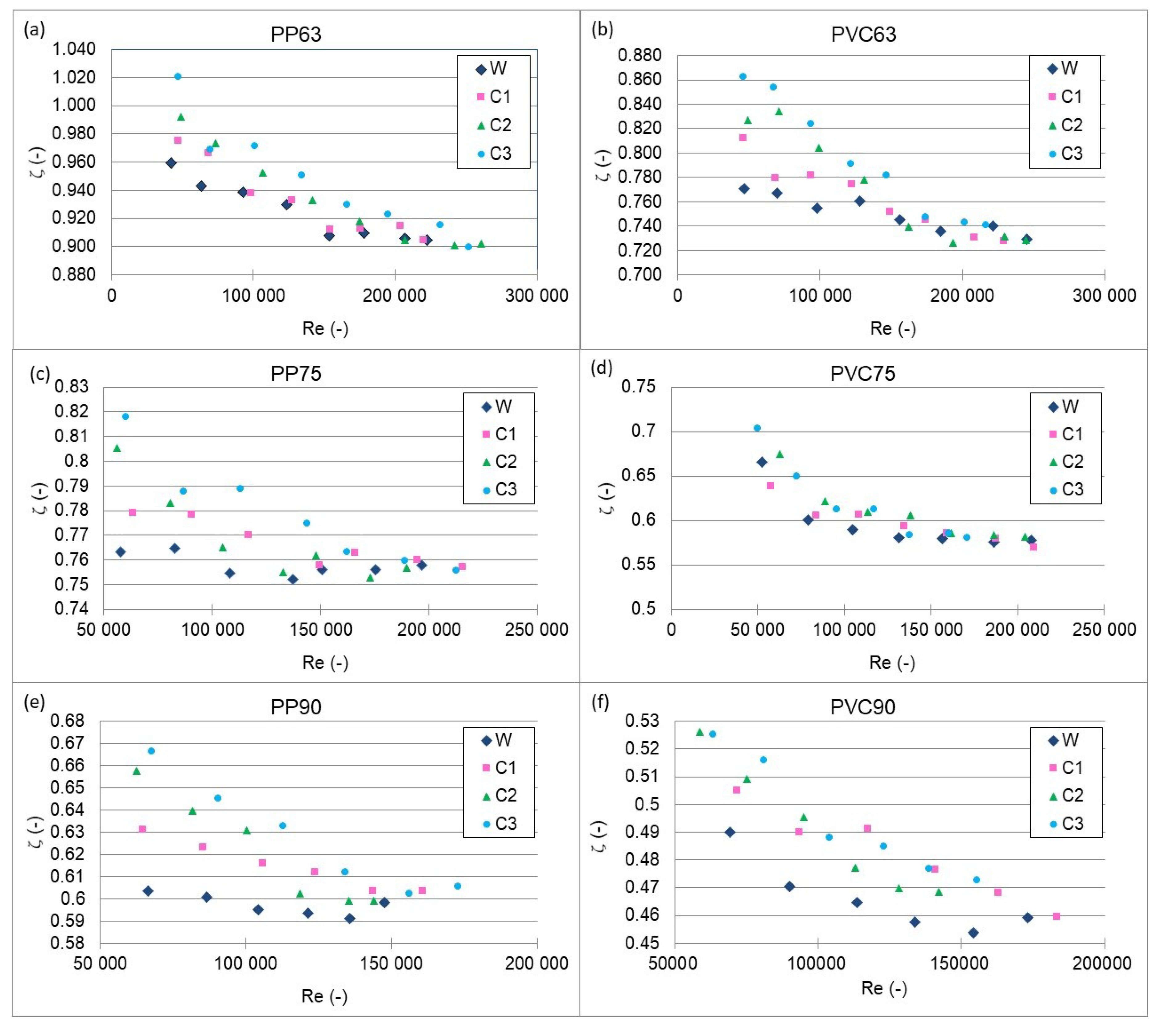
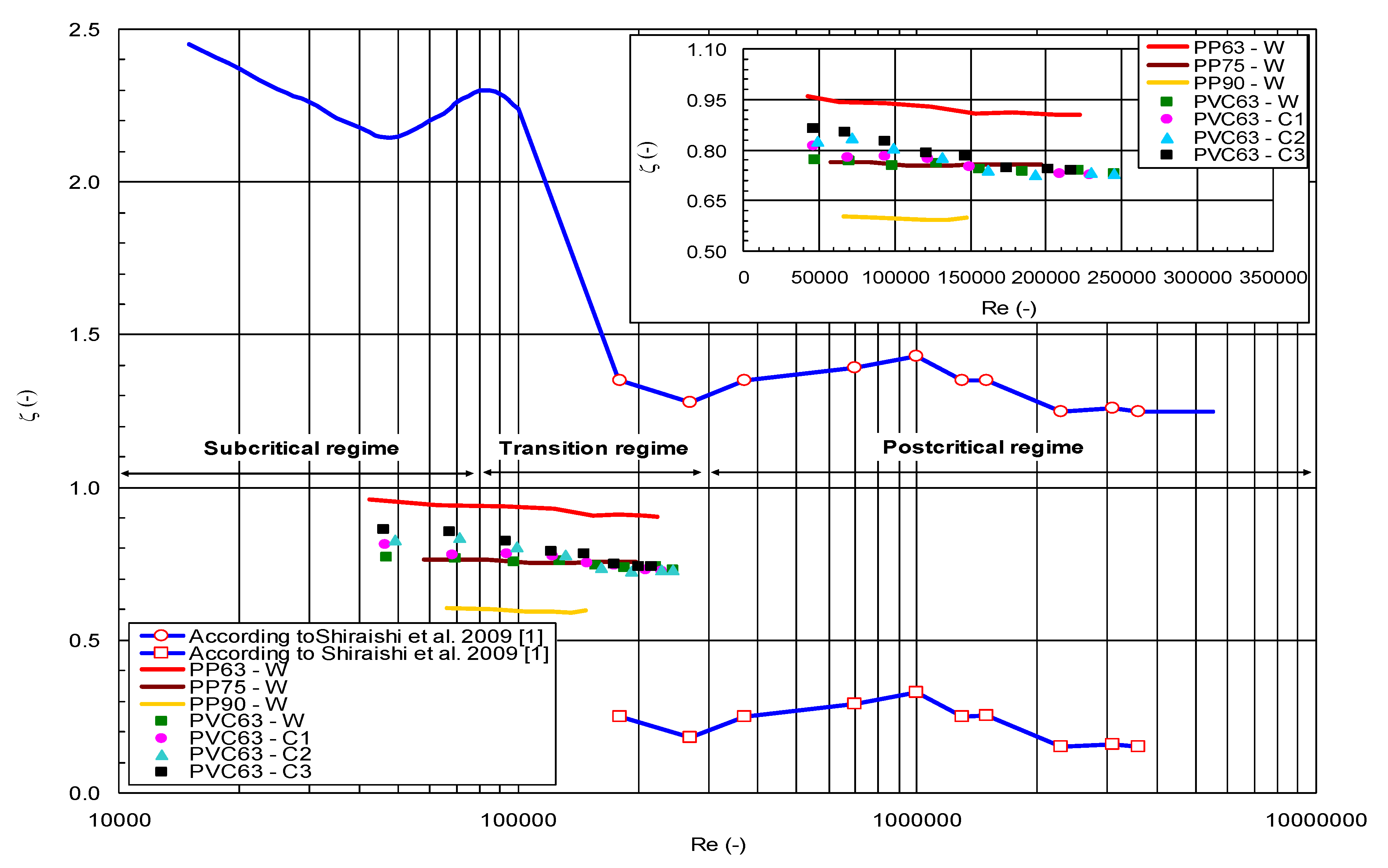
3.2. Results of Measurements

Measurements of variability in flow rate Q and the corresponding pressure loss p₁ – p₂ allowed us to determine the coefficient of minor head loss through elbow ζ. A graph showing minor head losses through elbow PVC90 as a function of flow rate (the right part of Equation (4)) is presented in Figure 3. The points on the graph form a ‘saw-like’ curve with two types of fluctuations. A first type is related to unstable operating conditions that always occur in closed-loop pump systems and are associated with pressure pulsation. A second type is connected with the pump’s adjusting to the new operating conditions altered by changing the degree of opening of the control valve, i.e., changing the flow rate of the liquid. This second type of fluctuations was not analyzed in this study; we calculated the coefficient of minor head losses through the elbows for a constant flow rate, as regulated by the control valve, after a sufficiently long time for the system to have reached a steady state. In the test conditions (Figure 3), lower flow rates required throttling of the pump by means of a control valve. This throttling is always the source of increased flux pulsations, which in this case intensified because the system worked in a loop, i.e., a pulsating stream flowing through the discharge line after a small suppression returned to the suction tube. At higher flow rates, this phenomenon was much smaller. The moment steady-state operating conditions had been reached, the memograph was switched on, which recorded the instantaneous values of the parameters. An analysis of the results recorded by the memograph showed that some of the observation points deviated from the remaining ones located along the function curve and showed an unambiguous tendency that followed from the given parameters: flow rate, sand concentration, pipeline diameter, type of elbow, and liquid temperature. These results were rejected on the basis of criterion ζav ± 2·σ (criterion range = 2 standard deviations from the mean) [38], i.e., a region that, according to the normal distribution, comprises 95.4% of the results.

An analysis of the distribution of coefficient ζ data points clearly shows that the coefficient assumes higher values at lower flow velocities. This increase becomes larger with an increasing concentration of sand in the mixture. As shown in Figure 2, sand did not deposit at the bottom of the pipe at a flow velocity of 1 m·s⁻¹, but at lower velocities, as follows from Newitt’s formula [36], sedimentation and dragging of sand along the bottom could have increased head loss, making the working conditions less stable. In the present study, analyses were performed at flow velocities V > 0.7 m·s⁻¹ to comply with the recommendations regarding design flow velocities in pressure sewerage systems [39,40]. The remaining results were excluded from modeling.

The results of measurements were substituted in Equation (7) to obtain head loss coefficients for the investigated elbows. Changes in these coefficients as a function of Reynolds number and sand concentration in the mixture are shown in Figure 4. For all samples, increases in flow velocity and elbow diameter, expressed here as Re, caused a drop in ζ. The differences were not big. In the case of water transport, the maximum decrease in ζ was about 5% for PP63, PVC63 and PVC90, about 1% for PP75 and PP90, and about 13% for PVC75. In all cases, an increase in the proportion of sand in the mixture increased head loss, which translated into higher values of coefficient ζ. Points on the graphs were calculated, using a descriptive statistic, from measurement points obtained in the stabilized flow range. Both Re and ζ are arithmetic means of a set of flow measurement points converted into Re, and head losses converted into ζ. The results from which the means were calculated came from measurement points obtained at a specific needle valve opening and a stabilized flow rate. Regarding clean water for PP63, PP75 and PP90 elbows with a flow rate of 0.7 m/s the value of ζ increased for C1—2.4%, C2—4.5%, C3—6.3% and for 2.5 m/s, 2.2%, 4.1% and 5.8% respectively. In the case of PVC63, PVC75 and PVC90 elbows the Reynolds number had a small effect on the ζ increments at different velocities. Therefore for the flow rate of 0.7 m/s and 2.5 m/s, the value of the ζ increased for C1—2.2%, C2—4.1%, C3—5.8%.

An analysis of the experimental results and the calculations leads to the conclusion that coefficient ζ for specific fittings should be determined by measurement methods. The values of minor head loss coefficients provided in technical catalogs of manufacturers and distributors of fittings often differ from the actual values, and values of coefficients for fittings of the same diameter can differ significantly across manufacturers, which is also shown in Figure 5.

The measurements reported in the present paper show that the velocity ranges used in pressure sewerage systems fall within two Reynolds regimes, subcritical and transition. The results of this study are not consistent with the results obtained by reference [1]. Their results show that the values of coefficient ζ for an elbow connected to an installation are within the range obtained separately for the installation and the elbow. This points to the important role of the joint between an elbow and a pipeline. Figure 5 shows that in the case of PP and PVC elbows, coefficient ζ is more strongly affected by elbow diameter than the concentration of sand in water. In the range of Reynolds number values of 2 × 10⁴–3 × 10⁴, obtained ζ = 1.1 for copper elbows [2].

When analyzing the problem of minor head losses, one should pay attention to the losses associated with the joint between the fitting and the straight sections of the pipeline. In real-life conditions, such joints also generate losses. The available literature reports do not provide information on whether the minor head loss coefficients ζ determined in those studies are values measured for the fitting alone or whether they also include losses generated at the joint between the fitting and the pipeline.

Studies that use specially prepared elbows [17,41] intended for measurement of specific parameters, cannot capture the phenomena which strongly affect head losses in real-life settings, for example in pressure sewers. Manufactured fittings always show some deviations from the correct dimensions, which results in additional turbulence. An important role is also played by the inner edge of the elbow (1) (Figure 6), which deflects the flow, as demonstrated by reference [13]. Such an edge is found in both PVC and PP elbows, but is prominently larger in the latter. This edge (Figure 7) substantially deflects flow on the inner side of the elbow and leads to the formation of vortices upstream of the elbow, as observed by other researchers [1,3,13]. The edge is formed where two cylindrical inlets meet, and covers half of the oblique cross-section of the elbow. The deflection is very sharp near the notch (3) (flow deflection angle of 90°); at distance D/4 from the notch flow deflection angle increases to 135°, and at distance D/2 the deflection disappears (flow deflection angle of 180°) (Figure 7). Such sharply sloping edges result from the fact that both PP and PVC elbows have a very low radius to diameter ratio, which in the investigated case was r/D = 0.52.

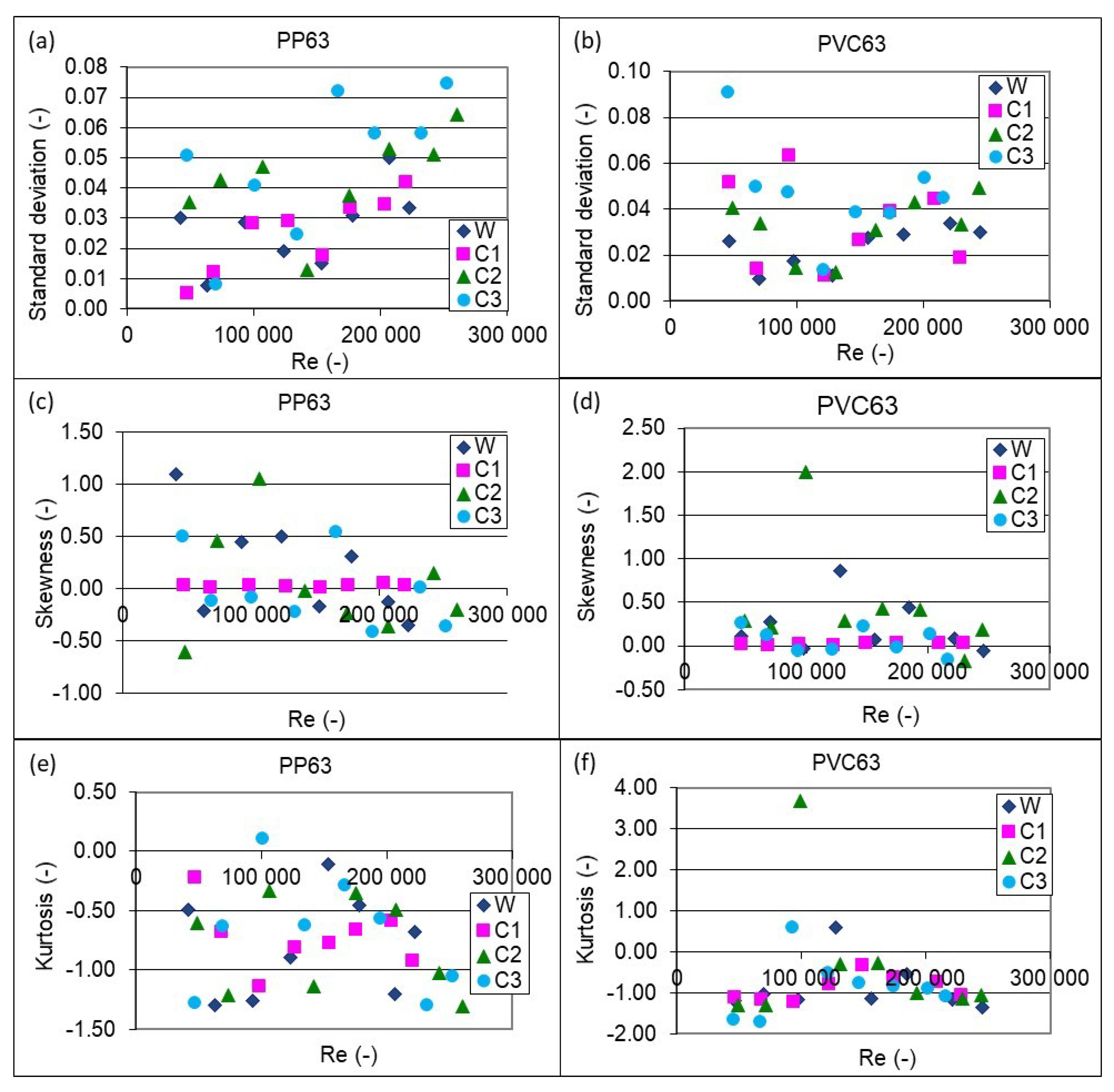
3.3. Statistical Analysis of Results

The fluctuations in pressure in loops of pipelines with a centrifugal pump are nicely characterized in Figure 8, which shows different standard deviations normalized by dynamic pressure [1]. The vast majority of positively skewed data points show a right-sided asymmetry, which means that the incidentally occurring large pressure fluctuations shift the mean to the right, whereby it becomes lower than the median. Negative kurtosis observed for most of the data points indicates a greater spread of points around the mean, i.e., the distributions are flatter than the normal distribution. No effect of sand concentration on the statistical measures analyzed was observed.

Pearson’s skewness coefficients were in the range of −0.5–0.5. In several cases, the distribution was very variable and had a tendency to either positive or negative asymmetry. These tendencies were more frequently observed at low flow velocities. The scatter of results was determined as the percentage ratio of standard deviation to mean. More stable operating conditions were found for PP elbows than for PVC ones. For PP elbows, scatter in Reynolds number defined in this way, for both W and C1–C3 was in the range of 0.15–2%, and scatter in coefficient ζ was 0.8–5.5%, with most scatter values of around 3%. Similarly, for PVC elbows, scatter in Reynolds number varied in the range of 0.8–3.2%, while scatter in coefficient ζ was 1.4–9.3%.

As shown in

Table 1. Means, medians and standard deviations of coefficients ζ for PP63 and PVC63 elbows at different R.

Medium	No.	W			C1			C2			C3
Elbow		ζav	ζmed	ζσ	ζav	ζmed	ζσ	ζav	ζmed	ζσ	ζav	ζmed	ζσ
PP63	1	0.905	0.909	0.034	0.905	0.915	0.042	0.902	0.915	0.064	0.899	0.920	0.075
	2	0.906	0.910	0.050	0.915	0.912	0.035	0.901	0.904	0.051	0.915	0.916	0.058
	3	0.910	0.909	0.031	0.913	0.914	0.033	0.905	0.905	0.053	0.923	0.928	0.058
	4	0.908	0.907	0.015	0.912	0.913	0.018	0.918	0.925	0.037	0.930	0.919	0.072
	5	0.930	0.924	0.019	0.933	0.938	0.029	0.933	0.932	0.013	0.951	0.952	0.025
	6	0.938	0.926	0.029	0.938	0.933	0.028	0.953	0.941	0.047	0.972	0.974	0.041
	7	0.943	0.944	0.008	0.967	0.972	0.012	0.973	0.961	0.043	0.969	0.968	0.008
	8	0.960	0.945	0.030	0.975	0.975	0.005	0.992	1.011	0.035	1.020	0.982	0.051
PVC63	1	0.729	0.729	0.030	0.728	0.725	0.019	0.729	0.738	0.049	0.741	0.747	0.045
	2	0.740	0.738	0.034	0.731	0.738	0.045	0.732	0.731	0.033	0.743	0.749	0.054
	3	0.736	0.728	0.029	0.745	0.742	0.039	0.726	0.710	0.043	0.748	0.754	0.038
	4	0.745	0.739	0.027	0.752	0.754	0.027	0.739	0.740	0.031	0.782	0.777	0.039
	5	0.761	0.759	0.011	0.774	0.773	0.011	0.778	0.777	0.013	0.791	0.794	0.013
	6	0.755	0.760	0.018	0.782	0.771	0.063	0.804	0.801	0.014	0.824	0.826	0.048
	7	0.767	0.765	0.010	0.779	0.783	0.014	0.834	0.830	0.034	0.854	0.836	0.050
	8	0.771	0.770	0.026	0.812	0.831	0.052	0.827	0.816	0.041	0.863	0.820	0.091

, in most cases, the distribution of results is close to symmetrical, as evidenced by the fact that medians ζmed are very similar to means ζav, and standard deviations ζσ are not very high. Table 1 shows selected results for PP63 and PVC63. The results in line 1 relate to the highest Re, and those in line 8 to the lowest Re. Re for the results ranged from about 2.4 × 10⁵ to 4.7 × 10⁴.

The tests showed that elbow diameter significantly influenced the minor head losses coefficient of the tested fittings. Minor head losses may also vary depending on the material from which the fitting is made (roughness), as well as the design of the fitting (e.g., segmented elbows, flex elbows, bend radius r, r/D ratio, etc.). This means that there are no universal values of the minor head loss coefficient applicable to various different hydraulic systems which use fittings made of different materials and transport different types of media. The present study provides some insight into the possibilities of designing pressure sewerage systems—information that cannot be found in product catalogs and standards, which mainly give values for elbows of small diameters. No data are available on minor head loss coefficients for fittings with larger diameters, which are commonly used in pressure sewerage systems.

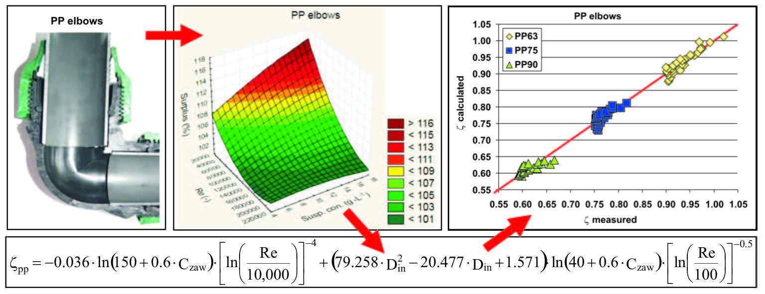
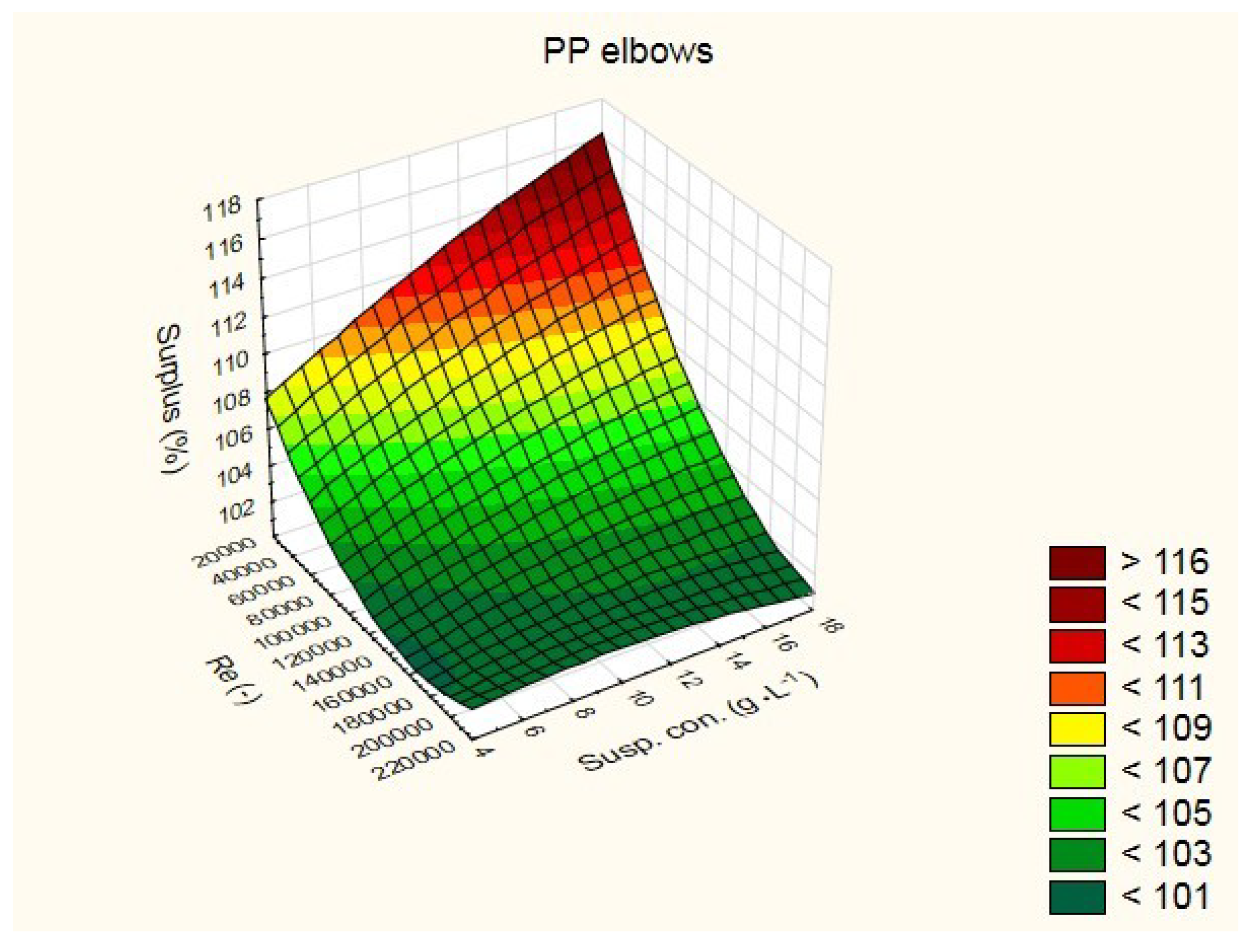
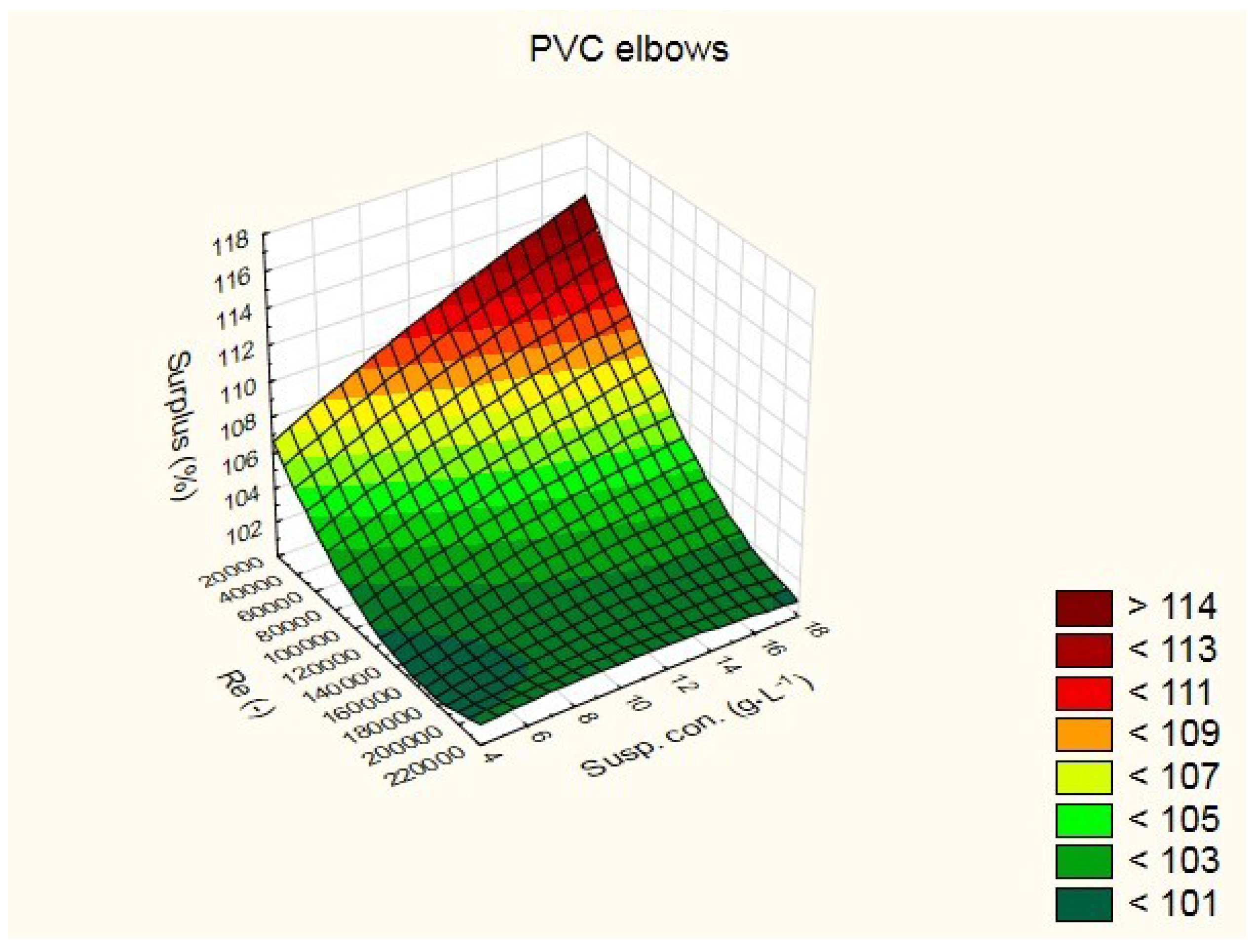
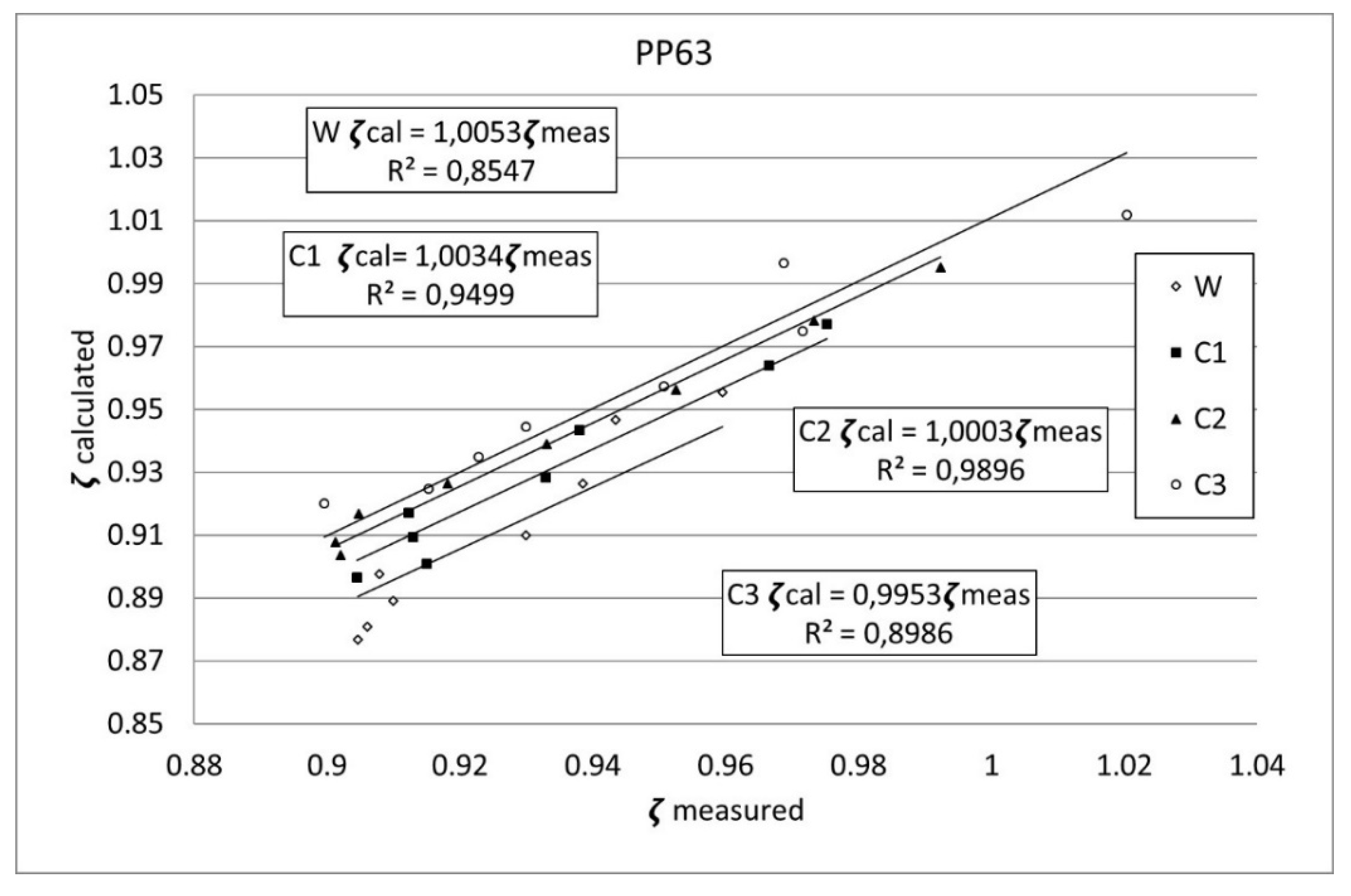
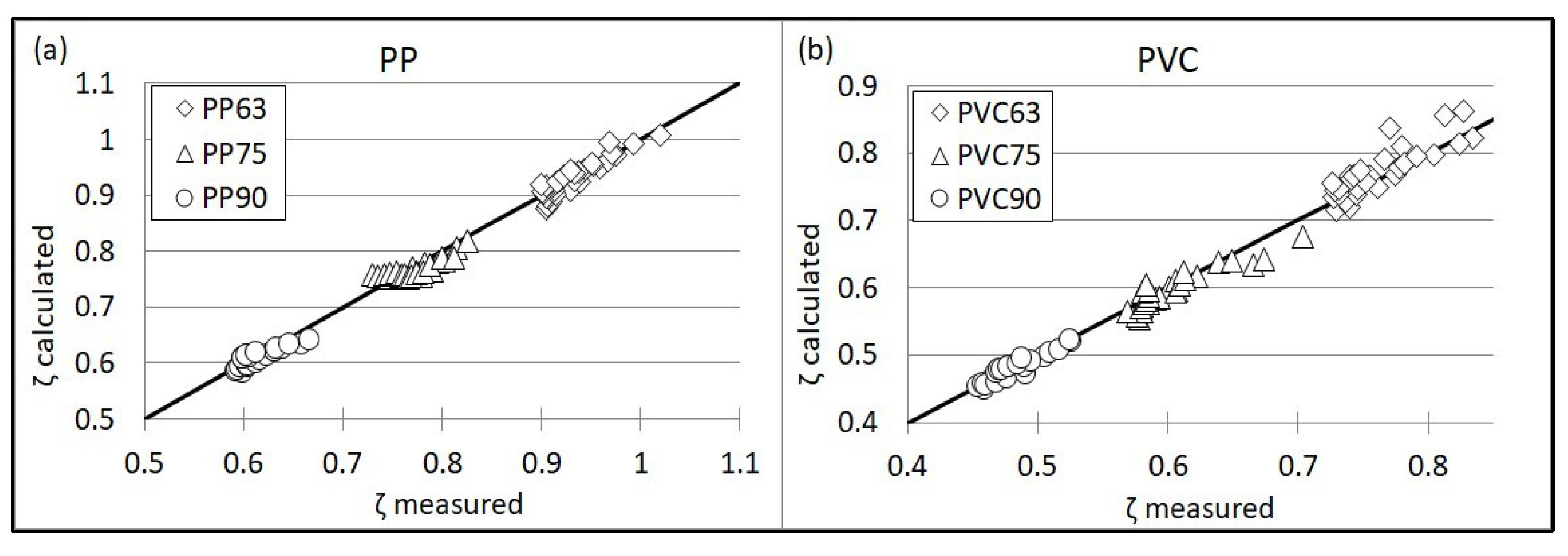
3.4. Appointment of Models for Calculation on the Minor Head Loss Coefficient for Elbows PP and PVC

To understand how sand concentration influences the operating conditions of a pump in a pressure sewage system, one can determine the increase in head loss relative to the transport of water alone. Figure 9 and Figure 10 show percent increases in head loss through PP and PVC elbows as a function of sand concentration and Reynolds number Re. The graphs show that the relative head losses for samples containing sand increase with an increase in sand concentration and a decrease in the Reynolds number.

As can be seen from Figure 9 and Figure 10, head losses increase along with the increase in flow velocity and sand concentration. Maximum head loss for the highest Re and sand concentration values was 116% for PP pipes and 114.5% for PVC pipes. Despite similar smoothness of the pipes, the increases were not the same due to differences in the internal structure of the fittings (different cross-sections, see Figure 9) and notches formed by pipe ends at the joint with the elbow (Figure 10). The surface diagrams shown in Figure 9 and Figure 10 suggest the possibility of modeling the variation of the local resistance coefficient as a function of the Reynolds number and the concentration of sand.

When analyzing the location and the variability of location of the observation points shown in Figure 8, we looked for a function that could describe the variability in coefficient ζ as a function of Reynolds number and concentration of suspended solids. Each set of points was very well approximated by the logarithmic function, both for water and water with sand. Determination coefficients R² were above 0.9. Incidentally, especially for elbow PP75, they reached a value of 0.8. Assuming that the partially generalized relationship would be based on the logarithmic function, Relationship (9) was found, which allows us to determine the minor head loss coefficient for the studied elbows as a function of Reynolds number Re and the concentration of suspended solids C_zaw. Relationship (9), although it has a general form and applies to all tested fittings, differs in the values of m and k factors, which should be considered separately for each elbow. The numerical values of these coefficients obtained in the calculations are given in

Table 2. Values of coefficients m and k for the model (Equation (7)) and ranges of the Reynolds number (applicability of the model).

Fitting	m	Value	k	Value	Remin	Remax
PP63	mPP63zaw	−0.031306	kPP63zaw	0.661078	4.2 × 104	2.6 × 105
PP75	mPP75zaw	−0.066786	kPP75zaw	0.546732	5.6 × 104	2.15 × 105
PP90	mPP90zaw	−0.0085	kPP90zaw	0.428871	6.2 × 104	1.7 × 105
PVC63	mPVC63zaw	−0.004077	kPVC63zaw	0.539926	4.6 × 104	2.5 × 105
PVC75	mPVC75zaw	−0.00892	kPVC75zaw	0.424447	4.9 × 104	2.1 × 105
PVC90	mPVC90zaw	−0.00973	kPVC90zaw	0.337607	5.9 × 104	1.8 × 105

. The last two columns show the range of applicability of the model, i.e., the range of Re for which the tests were performed. With regard to the concentration of suspended solids, the model is valid in the range of 0–15.73 g·L⁻¹, and sand concentrations should be substituted into the formula in these units (g·L⁻¹).

$${\zeta }^{zaw}=m\times \ln (150+0.6\times C_{zaw})\times {\left(\ln \frac{\mathrm{Re}}{\mathrm{10,000}}\right)}^{-4}+k\times \ln \left(40+0.6\times C_{zaw}\right)\times {\left(\ln \frac{\mathrm{Re}}{100}\right)}^{-0.5}$$

(9)

Goodness of fit of the model was assessed using graphs with the values obtained from the calculations plotted on the vertical axis and measured values plotted on the horizontal axis. An example of such a graph (for PP63) is presented in Figure 11. The obtained points were approximated by a linear function passing through the origin, which is why the correctness of the model was validated by the slope (direction coefficient) of the linear function. A linear function with a slope of 1.0 provides a good description of the experimental data. As can be seen from Figure 11, the direction coefficients are close to 1.0:1.0053 for water, 1.0034 for the C1, 1.0003 for the C2, and 0.9953 for the C3. The high values R² of the determination coefficient R² show that the fit is acceptable.

The next step was to look for a general equation that would take into account the diameter of the elbow. This was done by finding the functional relationship m = f(d) and k = f(d). The models were constructed using the cross validation method. The first model was constructed using the results for sand concentrations of 5.6 g·L⁻¹, 10.84 g∙L⁻¹, and 15.73 g∙L⁻¹; it was verified by calculating values ζ for C_zaw = 0, i.e., that of clear water. Then, the sums of squared errors were calculated using formula Σ(ζmodel − ζmeasurement)². These calculations were performed for each of the three concentrations of sand and for water. The total sum of squared errors across all observations, i.e., for sand concentrations of 0 g∙L⁻¹, 5.6 g·L⁻¹, 10.84 g·L⁻¹, and 15.73 g·L⁻¹, was used as the criterion of model fit. Next, a model was constructed for sand concentrations of 0 g∙L⁻¹, 10.84 g·L⁻¹, and 15.73 g·L⁻¹, and the model for the concentration of 5.6 g·L⁻¹ was verified. Further models were obtained using the 10.84 g·L⁻¹ and 15.73 g·L⁻¹ sand concentrations for verification, and the remaining series of results were used to construct models. In this way, four models were obtained for each pipeline diameter, and the one that had the smallest total sum of squared errors was selected as the final model. The maximum differences between the sums of squared errors between the individual models were 14.6% for PP fittings and 13.5% for PVC fittings. The remaining ones had lower values ranging from 2.6% to 9.5%. The models with the best fit for each type of material are summarized in Equations (10) and (11):

$${\zeta }_{PP}=-0.036\cdot \ln (150+0.6\cdot C_{zaw})\cdot {\left[\ln \left(\frac{\mathrm{Re}}{10,000}\right)\right]}^{-4}+\left(79.258·D_{in}^2-20.477·D_{in}+1.571\right)·\ln \left(40+0.6·C_{zaw}\right)·{\left[\ln \left(\frac{\mathrm{Re}}{100}\right)\right]}^{-0.5}$$

(10)

$${\zeta }_{PVC}=0.038\cdot \ln (150+0.6\cdot C_{zaw})\cdot {\left[\ln \left(\frac{\mathrm{Re}}{10,000}\right)\right]}^{-4}+\left(229.66·D_{in}^2-40.388·D_{in}+12.096\right)·\ln \left(40+0.6·C_{zaw}\right)·{\left[\ln \left(\frac{\mathrm{Re}}{100}\right)\right]}^{-0.5}$$

(11)

In both equations, inner pipe diameter D_in is expressed in ‘meters’ and sand concentration C_zaw in g·L⁻¹.

Figure 12, which shows agreement between measured and calculated coefficients ζ, confirms the good choice of the model equation.

Figure 12 shows the significant influence of pipeline diameter on the value of minor head loss coefficient ζ. The values of ζ are ca. 0.95 for PP63, ca. 0.78 for PP75, and ca. 0.62 for PP90. The respective values for PVC are 0.8, 0.6, and 0.48. The differences between PVC and PP elbows are a consequence of the presence of structural notches in PP fittings and the distinct ways in which the two types of fittings are connected to pipe sections. The coefficients of determination for the particular groups of observation points shown in Figure 11 were: PP63 0.863; PP75 0.704; PP90 0.768; PVC63 0.791; PVC75 0.859; and PVC90 0.897, which testifies to the very good fit of the models to experimental data.

The effect of sand concentration on the value of minor head loss coefficient ζ was determined using the null hypothesis that there is no significant difference in the values of the coefficient between the flow of water and the flow of water with a given concentration of sand. The results were considered significant at α = 0.05. P values were calculated using the two-tailed Student’s t-test. It was shown that the null hypothesis should be rejected, which may indicate that the effect of sand concentrations in the range of 0–15.73 g·L⁻¹ was statistically significant.

4. Conclusions

The following conclusions were formulated on the basis of the results obtained in the present study:

1. An increase in elbow diameter is accompanied by a decrease in minor head loss coefficient ζ. It is an incorrect practice, often found in product catalogs, to provide values of minor head loss coefficients in a general form. Separate values should always be provided for fittings of different diameters.

2. Minor head loss coefficient ζ is not a constant value. It depends quite strongly on the Reynolds number, especially at low flow velocities. An increase in velocity (Reynolds number) results in a decrease in the value of coefficient ζ. The actual relationship is more complex, and as shown in this study, ζ depends on Re, the concentration of suspended solids, and the diameter of the fitting. It was found that the influence of sand, in the investigated range of concentrations, on minor head losses was statistically significant.

3. The values of minor head loss coefficients given in the literature often diverge from real values and can only be used for making estimates. When precise calculations are needed, in particular in the case of complex hydraulic systems, minor head loss coefficients should be determined experimentally.

4. At flow velocities below 0.7 m/s, a marked increase in head loss is observed especially for the samples containing sand. This is associated with sedimentation of sand at the bottom of the pipes. The results are not very stable, which is why they were not used in the development of the calculation model.

5. Relative pressure losses in the samples with sand compared to the water decrease along with increasing Reynolds number. On average, for all samples containing suspended solids, they are 2.1% for every 5 g of sand·dm⁻³ higher in relation to water for PP elbows and 2.0% for PVC elbows. These differences, however, are so small that coefficients determined for water can be used to make approximate calculations.

6. As shown, use of data from large-scope tests allows to develop a mathematical model that makes it possible to automate calculations and predict head losses in more complex hydraulic systems. The obtained models show a very good fit, which, depending on the diameter of the fittings, ranges between 0.704–0.860 for PP, and 0.791–0.897 for PVC.

References

1. Shiraishi, T.; Watakabe, H.; Sago, H.; Yamanao, H. Pressure fluctuation characteristics of the short-radius elbow pipe for FBR in the postcritical Reynolds regime. J. Fluid Sci. Technol. 2009, 4, 430–441. [Google Scholar] [CrossRef]
2. Ma, Z.W.; Zhang, P. Pressure drops and loss coefficients of a phase change material slurry in pipe fittings. Int. J. Refrig. 2012, 35, 991–1002. [Google Scholar] [CrossRef]
3. Ono, A.; Kimura, N.; Kamide, H.; Tobita, A. Influence of elbow curvature on flow structure at elbow outlet under high Reynolds number condition. Nucl. Eng. Des. 2011, 241, 4409–4419. [Google Scholar] [CrossRef]
4. Shi, X.J.; Zhang, P. Two-phase flow and heat transfer characteristics of tetra-n-butyl aminium bromide clathrate hydrate slurry in horizontal 90° pipe and U-pipe. Int. J. Heat Mass Transf. 2016, 97, 364–378. [Google Scholar] [CrossRef]
5. Ikarashi, Y.; Taguchi, S.; Yamagata, T.; Fujisawa, N. Mass and momentum transfer characteristics in and downstream of 90° elbow. Int. J. Heat Mass Transf. 2017, 107, 1085–1093. [Google Scholar] [CrossRef]
6. Dutta, P.; Saha, S.K.; Nandi, N.; Pal, N. Numerical study on flow separation in 90° pipe bend under high Reynolds number by k-ε modelling. Eng. Sci. Technol. Int. J. 2016, 19, 904–910. [Google Scholar] [CrossRef]
7. Duarte, C.A.R.; Souza, F.J.; de Vasconcelos Salvo, R.; dos Santos, V.F. The role of inter-particle collisions in elbow erosion. Int. J. Multiph. Flow 2017, 89, 1–22. [Google Scholar] [CrossRef]
8. Vieira, R.E.; Parsi, M.; Zahedi, P.; McLaury, B.S.; Shirazi, S.A. Ultrasonic measurements of sand particle erosion under upward multiphase annular flow conditions in a vertical-horizontal bend. Int. J. Multiph. Flow 2017, 93, 48–62. [Google Scholar] [CrossRef]
9. Kalenik, M. Empirical formulas for calculation of negative pressure difference in vacuum pipelines. Water 2015, 7, 5284–5304. [Google Scholar] [CrossRef]
10. Qiao, S.; Kim, S. Interfacial area transport across a 90° vertical-upward elbow in air–water bubbly two-phase flow. Int. J. Multiph. Flow 2016, 85, 110–122. [Google Scholar] [CrossRef]
11. Yadaw, M.S.; Kim, S.; Tien, K.; Bajorek, S.M. Experiments on geometric effects of 90-degree vertical-upward elbow in air water two-phase flow. Int. J. Multiph. Flow 2014, 65, 98–107. [Google Scholar] [CrossRef]
12. Yadaw, M.S.; Worosz, T.; Kim, S.; Tien, K.; Bajorek, S.M. Characterization of the dissipation of elbow effects in bubbly two-phase flows. Int. J. Multiph. Flow 2014, 66, 101–109. [Google Scholar] [CrossRef]
13. Rohring, R.; Jakirlić, S.; Tropea, C. Comparative computational study of turbulent flow in a 90° pipe elbow. Int. J. Heat Fluid Flow 2015, 55, 120–131. [Google Scholar] [CrossRef]
14. Yoo, D.H.; Singh, V.P. Explicit design of commercial pipes with secondary losses. J. Hydro-Environ. Res. 2010, 4, 37–45. [Google Scholar] [CrossRef]
15. Li, A.; Chen, X.; Chen, L.; Gao, R. Study on local drag reduction effects of wedge-shaped components in elbow and T-junction close-coupled pipes. Build. Simul. 2014, 7, 175–184. [Google Scholar] [CrossRef]
16. Yuki, K.; Hasegawa, S.; Sato, T.; Hoshizume, H.; Aizawa, K.; Yamano, H. Matched refractive-index PIV visualization of complex flow structure in a three-dimentionally connected dual elbow. Nucl. Eng. Des. 2011, 241, 4544–4550. [Google Scholar] [CrossRef]
17. Ebara, S.; Takamura, H.; Hoshizume, H.; Yamano, H. Characteristics of flow field and pressure fluctuation in complex turbulent flow in the third elbow of a triple elbow piping with small curvature radius in three-dimensional layout. Int. J. Hydrogen Energy 2016, 41, 7139–7145. [Google Scholar] [CrossRef]
18. Basset, M.; Winterbone, D.; Pearson, R. Calculation of steady flow pressure loss coefficients for pipe junctions. Proc. Inst. Mech. Eng. Part C J. Mech. Eng. Sci. 2001, 861–881. [Google Scholar] [CrossRef]
19. Cisowska, I.; Kotowski, A. Studies of hydraulic resistance in polypropylene pipes and pipe fittings. Found. Civ. Environ. Eng. 2006, 8, 37–57. [Google Scholar]
20. Gietka, N.N. Experimental analysis of local resistance coefficients on elbows in multilayer duct systems. Acta Sci. Pol. Formatio Circumiectus 2015, 14, 47–56. [Google Scholar] [CrossRef]
21. Siwiec, T.; Morawski, D.; Karaban, G. Experimental tests of head losses in welded plastic fittings. Gaz Woda Technika Sanitarna 2002, 2, 49–68. (In Polish) [Google Scholar]
22. Nawrot, T.; Matz, R.; Błażejewski, R.; Spychała, M. A case study of a small diameter gravity sewerage system in Zolkiewka Commune, Poland. Water 2018, 10, 1358. [Google Scholar] [CrossRef]
23. Gopaliya, M.K.; Kaushal, D.R. Modeling of sand-water slurry flow through horizontal pipe using CFD. J. Hydrol. Hydromech. 2016, 64, 261–272. [Google Scholar] [CrossRef]
24. Vlasak, P.; Chara, Z.; Krupička, J.; Konfršt, J. Experimental investigation of coarse particles-water mixture flow in horizontal and inclined pipes. J. Hydrol. Hydromech. 2014, 62, 241–247. [Google Scholar] [CrossRef]
25. Assefa, K.M.; Kausha, D.R. A comparative study of friction factor correlations for high concentrate slurry flow in smooth pipes. J. Hydrol. Hydromech. 2015, 63, 13–20. [Google Scholar] [CrossRef]
26. Csizmadia, P.; Hos, C. CFD-based estimation and experiments on the loss coefficient for Bingham and power-law fluids through diffusers and elbows. Comput. Fluids 2014, 99, 116–123. [Google Scholar] [CrossRef]
27. Kalenik, M.; Witowska, B. Research of local hydraulic resistance in PVC fittings. ACTA Scientiarum Polonorium. Architectura 2007, 6, 15–24. (In Polish) [Google Scholar]
28. Weinerowska-Bords, K. Experimental analysis of local energy loss coefficients for selected fittings and connectors in polymeric multilayer pipe systems. Instal 2014, 6, 42–49. (In Polish) [Google Scholar]
29. Liu, M.; Duan, Y.F. Resistance properties of coal–water slurry flowing through local piping fittings. Exp. Therm. Fluid Sci. 2009, 33, 828–837. [Google Scholar] [CrossRef]
30. Pliżga, O.; Kowalska, B.; Musz-Pomorska, A. Laboratory and numerical studies of water flow through selected fittings installed at copper pipelines. Annu. Set Environ. Prot. 2016, 18, 873–884. [Google Scholar]
31. Li, Y.; Wang, C.; Ha, M. Experimental determination of local resistance coefficient of sudden expansion tube. Energy Power Eng. 2015, 7, 154–159. [Google Scholar] [CrossRef]
32. PN-EN 1267:2012. Industrial Valves—Test of Flow Resistance Using Water as Test Fluid. Polish Standard. Available online: http://sklep.pkn.pl/pn-en-1267-2012e.html (accessed on 18 March 2016).
33. PN-EN 12880:2004. Characterization of Sludges. Determination of Dry Residue and Water Content. Polish Standard. Available online: http://sklep.pkn.pl/pn-en-12880-2002e.html (accessed on 18 March 2016).
34. Siwiec, T.; Wichowski, P.; Kalenik, M.; Morawski, D. Comparative analyse formulas for calculation head coefficient in plastic pipes with water and wastewater flow. Instal 2012, 7–8, 52–57. (In Polish) [Google Scholar]
35. Jeż, P.; Książyński, K.; Gręplowska, Z. Tables for Hydraulic Calculations; Cracow University of Technology: Cracow, Poland, 1998. (In Polish) [Google Scholar]
36. Dziubiński, M.; Prywer, J. Mechanics of Two-Phase Fluids; WNT: Warsaw, Poland, 2009. (In Polish) [Google Scholar]
37. Wilson, K.C.; Addie, G.R.; Sellgren, A.; Clift, R. Slurry Transport Using Centrifugal Pumps, 3rd ed.; Springer: Berlin, Germany, 2006. [Google Scholar]
38. Zięba, A. Data Analysis in Science and Technology; PWN: Warsaw, Poland, 2013. (In Polish) [Google Scholar]
39. PN EN 16932-2:2018. Drain and Sewer Systems Outside Buildings.Pumping Systems. Positive Pressure Systems. Available online: http://sklep.pkn.pl/pn-en-16932-2-2018-05e.html (accessed on 18 March 2016).
40. Wichowski, P.; Zalewska, K. Experimental studies on removal of mineral suspension from siphons in rain water pipelines. Annu. Set Environ. Prot. 2015, 17, 1642–1659. (In Polish) [Google Scholar]
41. Mizutani, J.; Ebara, S.; Hashizume, H. Evaluation of influence of the inlet swirling flow on the flow field in the triple elbow system. Int. J. Hydrogen Energy 2016, 41, 7233–7238. [Google Scholar] [CrossRef]
Figure 1. Schematic of the test stand for measuring minor head losses through elbows: 1—elbow, 2—thermometer, 3—pipe supplying sewage to the tank, 4—sewage tank, 5—pipe channeling sewage from the tank, 6—sewage pump, 7—needle valve, 8—sewage flow meter, 9, 10 and 12—control cable, 11—data recorder, 13—differential pressure meter, 1–1; 2–2—test cross-sections, L1, L2—distance of measuring cross-sections to the elbow.
Water 11 00828 g001
Figure 2. View of mixtures of water with different concentrations of sand C1, C2, and C3; W—water.
Water 11 00828 g002
Figure 3. Minor head loss coefficient ζ for a PVC90 elbow as a function of water flow velocity and three concentrations of water-and-sand mixture.
Water 11 00828 g003
Figure 4. Values of coefficient ζ as a function of Reynolds number Re and concentration of sand for the test elbows. Elbows: (a,b)—diameter 63 mm, (c,d)—diameter 75 mm, (e,f)—diameter 90 mm.
Water 11 00828 g004
Figure 5. Comparison of experimental data for ζ with the correlation found by Shiraishi et al. (2009) [1].
Water 11 00828 g005
Figure 6. Longitudinal section of the test elbows: 1—inner edge of the elbow, 2—edge of the joint, 3—inner notch.
Water 11 00828 g006
Figure 7. Flow deflection angle on the inner edge of an elbow.
Water 11 00828 g007
Figure 8. Standard deviation, skewness, and kurtosis as a function of Re for selected PP and PVC elbows. Elbows: (a,b)—diameter 63 mm, (c,d)—diameter 75 mm, (e,f)—diameter 90 mm.
Water 11 00828 g008
Figure 9. Increase in head loss through PP elbows for water-sand mixtures compared to clear water, as a function of sand concentration and Reynolds number.
Water 11 00828 g009
Figure 10. Increase in head loss through PVC elbows for water-sand mixtures compared to clear water, as a function of sand concentration and Reynolds number.
Water 11 00828 g010
Figure 11. Verification of the correctness of the adopted model for the PP63 elbow.
Water 11 00828 g011
Figure 12. Verification of the correctness of the adopted model for PP (a) and PVC (b) elbows as a function of diameter d, concentration of suspended solids C, and Reynolds number Re.
Water 11 00828 g012