1. Introduction
Debris flows in southwestern China are sometimes initiated when soil is mobilized by a high enough water flow. Methods used to study debris flow initiation include field observation [
1,
2,
3], laboratory flume experiments [
4,
5,
6], statistical methods, and theoretical derivation [
7,
8,
9]. Debris flow occurs frequently in catchments which have well-developed main channels and tributary gullies. The evolution of debris flows after an earthquake often occurs with increased coarse material and higher frictional resistance, which decreases their frequency and increases difficulty in debris flow identification or prediction. According to the characteristics of debris flows, Tang et al. (2008) [
10] pointed out that the critical precipitation and initial discharge can be used as indicators for the initiation of debris flows. The discharge per unit width (m
3/s·m) was taken as the available indicator of debris flow initiation [
2,
7,
9], due to the fact that the discharge, in combination with parameters such as debris grain size, slope angle, and sediment concentration, can be obtained and applied to scientific research, prediction, and practice.
Some flume experiment simulations of runoff discharge have been performed [
6] to understand impact of gully bed gradient and average particle size. Coe et al. (2008) [
2] verified the accuracy of the critical discharge of overland runoff based on field observation data. However, their results were obviously different from the source of the Wenchuan earthquake area; deposit heterogeneity should be considered when critical debris flow discharge data are computed. The same average grain size or percentage of particles less than 10 mm in diameter in the flume test had an influence on Wenchuan earthquake area. Severe erosion and transport led to high solid concentrations, generating debris flows. [
11]. The critical discharge can be simulated in serial tests and calculated in terms of its relationships, avoiding analyzing hydrodynamic force by using the size and slope. The parameter of critical discharge could be an effective criterion to assess channel sediment instability.
According to the distributed hydrological models such as the Hydrologic Engineering Center’s Hydrologic Modeling System (HEC-HMS) [
12] and the Integrated Hydrologic Model (inHM) [
13], the surface or subsurface hydrologic responses can be simulated. With the surface runoff discharge, two methods, (1) Manning’s formula [
14,
15,
16] or (2) Shen’s method [
17], can be used to calculate the discharge of debris flow. The volumetric concentration of solid particles of debris flow can also be determined by internal friction angle and inclination [
18,
19]. Hydrological response analysis on critical precipitation and discharge has thus become more available; meanwhile, predictions on debris flow discharge can feasibly be made. Rainfall, as an important factor formulized as rainfall intensity-duration (I-D) curve for debris flow initiation, has been frequently used [
2,
20,
21,
22]. Rainfall patterns in the Wenchuan earthquake area [
21] have shown that the runoff coefficient and peak discharge of an instantaneous heavy rainfall can be 5 to 6 times higher compared than that of a rainfall with uniform intensity [
23]. As a potential factor of initiation, the same magnitude of cumulative rainfall may lead to different water discharges when the rainfall pattern is different.
For rainfall pattern estimation, Huff (1967, 1990) [
24,
25] first divided the precipitation process into four phases, and the National Oceanic and Atmospheric Administration (NOAA ) published the Huff curve in America [
26], while Azli et al. (2010) [
27] and Domen et al. (2016) [
28] studied the temporal characteristics of rainfall around China, Peninsular Malaysia, and Slovenia based on the Huff curve. To reveal how confluence in the catchment changed with different rainfall patterns, the rainfall data used in this paper were gathered from three rainfall stations located on Longmen Mountain (
Table 1), and the meteorology of these stations was similar to that of a station in Yuzi River in Yingxiu.
This study obtained the rainfall patterns statistically. The corresponding runoff discharge and debris flow discharge were calculated based on distributed hydrological modeling, field surveys, and empirical relationships. Further prediction of rainfall threshold combined with rainfall patterns is presented. A direct survey of the debris flow on 26 July 2016 in Xiongmao Ravine and 165 effective rainfall events were collected.
2. Study Area
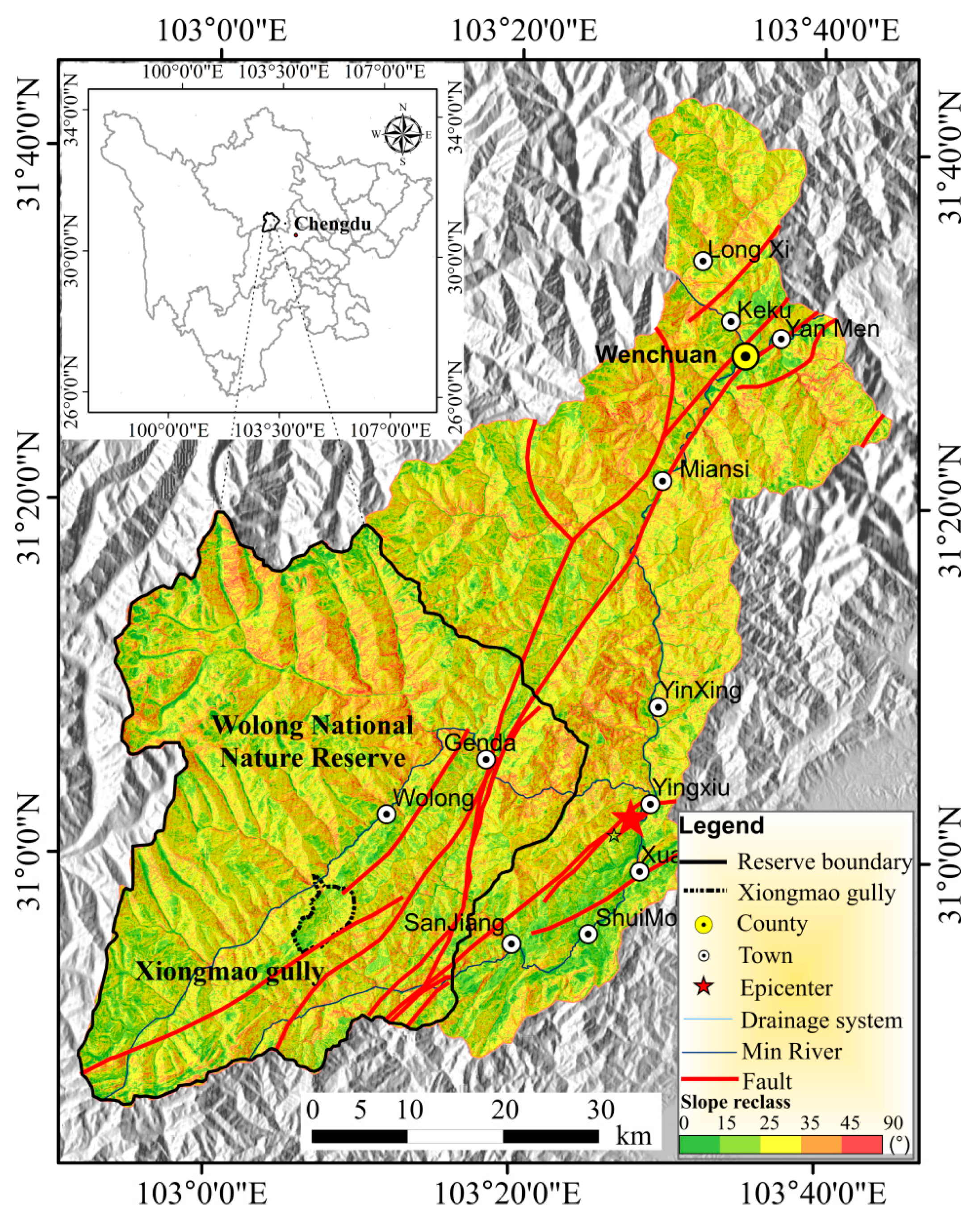
On 12 May 2008, Yinxiu, a town in Wenchuan County, located on the fault zone of Longmen Mountain, was hit by a Richter 8.0 earthquake. The straight-line distance of the study area to the epicenter was 32.3 km (
Figure 1). The earthquake heavily damaged the buildings and infrastructure of Wolong town in Wenchuan County, and loosened the mountain surface, resulting in collapse and landslide and providing abundant loose sources for the debris flow.
Xiongmao Gully, located in the Wolong nature reserves, southwest of Wolong, Wenchuan County, Sichuan Province, is the primary tributary on the right bank of Yuzi river. The average longitudinal length of the gully is 8.8km, average width is 3.4 km, average longitudinal grade is 169.9‰, and the catchment area is 23.6 km
2. Additionally, the highest elevation located at the southwest outlet of the gully is 3600 m; the lowest one at the junction between the outlet and Yuzi River is 2105 m. The upstream catchment contains six branches with lengths from 0.9 to 2.4 km and longitudinal gradients from 15% to 35% (
Figure 1 and
Figure 2).
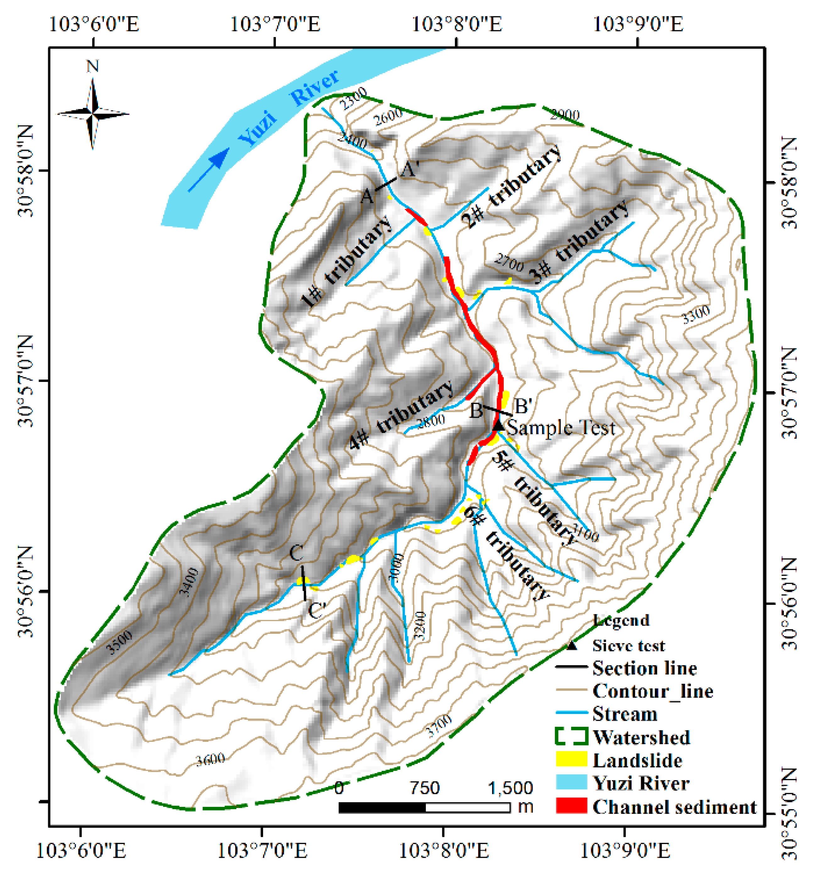
The catchment consists of carbonaceous phyllites, sandy phyllites, slates, and crystalline limestones. The upstream topography of the gully is U-shaped and the vegetation consists mainly of shrubs; the downstream valley is roughly V-shaped, with steep slopes on both sides and well-developed cliffs with gradients of 50°–70°. The channel sediment (red areas in
Figure 2) in the midstream and collapse accumulation (yellow areas in
Figure 2) in the upstream represented the majority of solid material; midstream erosion was located on the red areas, and the main initiation thus occurred along Tributary 6 and Tributary 5.
Debris flows broke out in Xiongmao Gully in 1995, 1998, and May 2004, destroying large areas of agricultural land, but with no casualties reported. The Wenchuan earthquake triggered landslides, producing a large volume of debris deposits in the upstream catchment, providing an abundant source of material for debris flows.
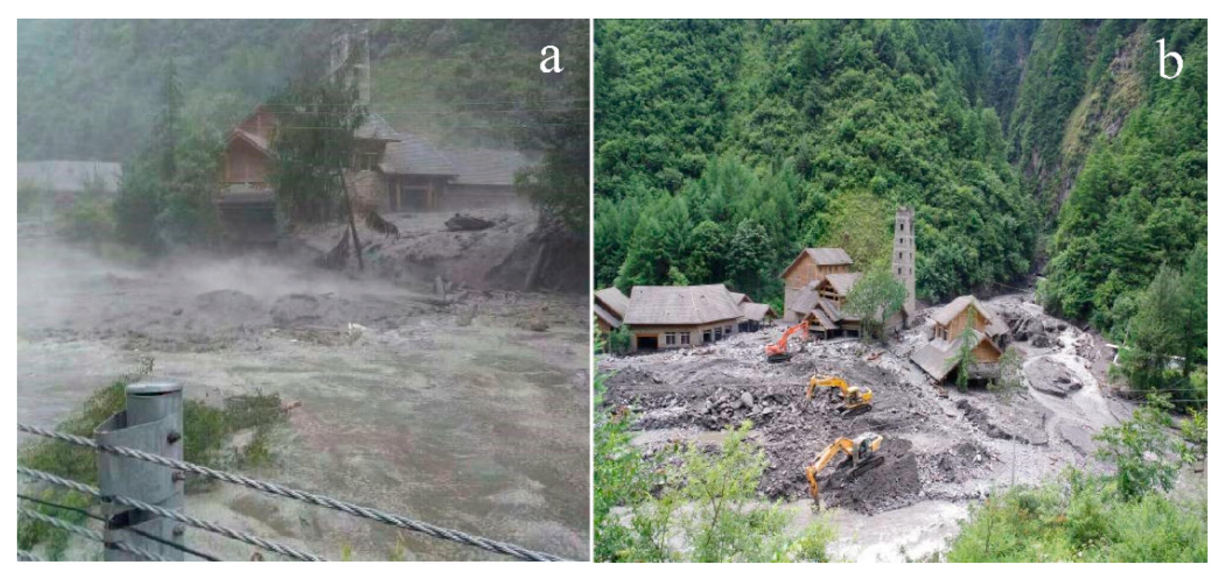
On 26 July 2016, a sudden rainstorm in Wolong with a cumulative rainfall of about 70 mm between 14:00 and 16:00 increased the water discharge of Yuzi River significantly and, until 16:00, debris flows occurred in Xiongmao Gully, and the debris rushed out and flooded roads, blocking the tributaries in the catchment and Yuzi river, generating tremendous economic damage to the local people and infrastructure (
Figure 3). According to the Manual of Floods in Small Watersheds of Sichuan Province, the rainfall within 24h at frequencies of 1%, 2%, 5%, and 10% in Xiongmao Gully was 211.5 mm, 190.8 mm, 162.0 mm, and 139.5 mm, and the rainfall within 6 h was 127.4 mm, 113.7 mm, 94.6 mm, and 79.4 mm respectively.
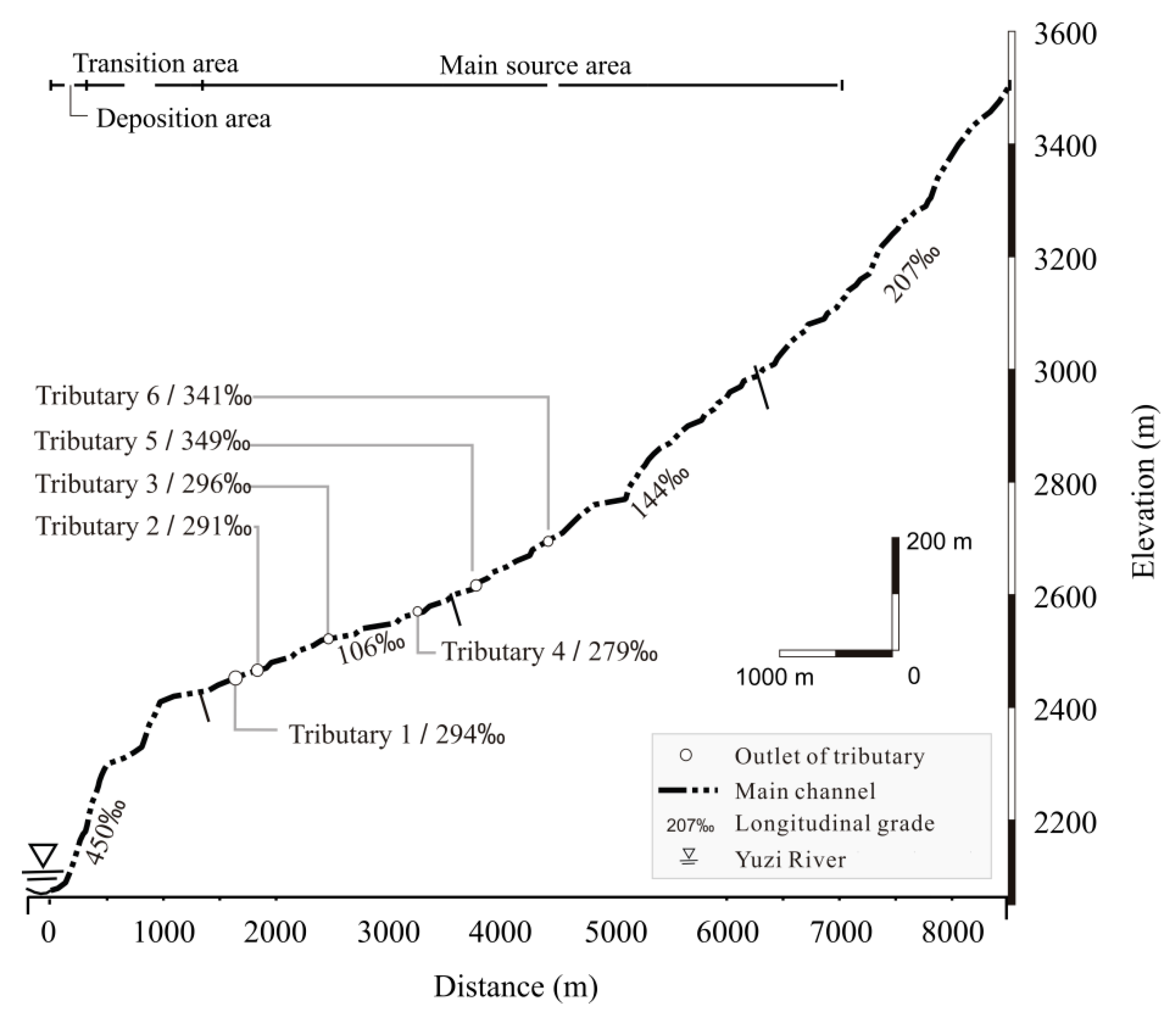
The longitudinal profile of Xiongmao Gully revealed that the whole gully gradually slowed due to the reduced upstream longitudinal gradient from the original 207‰ to 106–144‰. In particular, the reduced longitudinal gradient of the original area led to the debris being readily deposited and decreased the debris flow velocity. At the downstream transition area, the longitudinal gradient became abrupt, reaching a maximum of 450‰, which drove an outrush of debris into Yuzi River (
Figure 4).
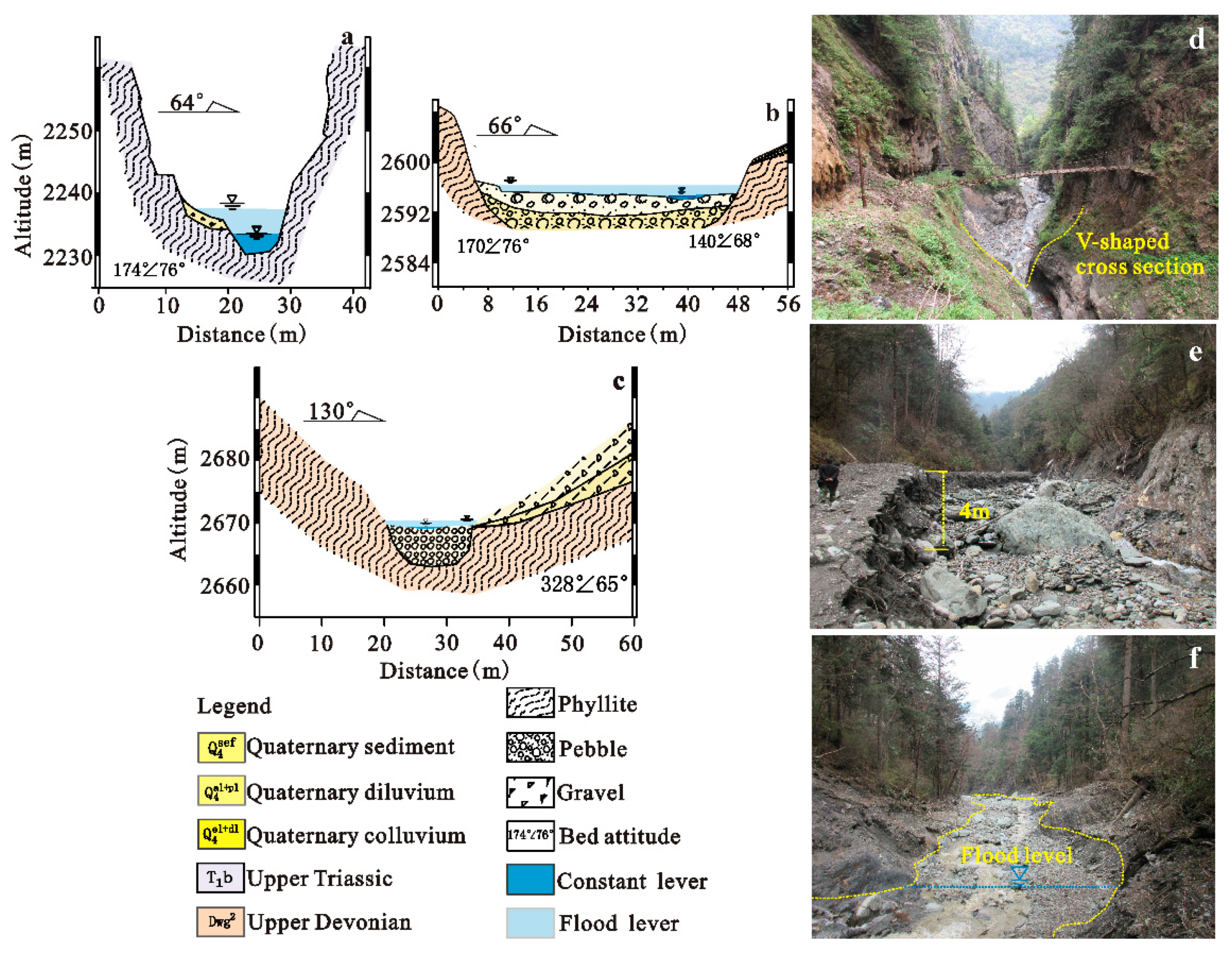
Xiongmao Gully can be divided into source area and transition and accumulation zones.
Figure 5a,b shows cross-sections of the upper and lower parts of the transition zone, while
Figure 5c shows it through the source area. Photos of the transition zone with a deep gully, the sediment initiation area, and flood flow area are shown in
Figure 5d–f, respectively.
The gully length of the transition zone is about 0.83 km, with an average longitudinal grade of about 38% and 45% at the maximum. In this section, the gully had a V-shape with a width of 3 to 8 m. The channel bed was heavily eroded, and both sides were steep rock slopes without landslides (
Figure 5a,d).
The topography of source area was U-shaped, with bank slopes on both sides and abundant unconsolidated material. Most of the slopes were eroded as slightly bank cutting (
Figure 5c,f). The upstream valley was covered by a thin layer of weathered deposits and dense vegetation. This region consisted of bare rock slopes and, therefore, could generate a large volume of run-off water for debris flow initiation.
It was known from the source distribution of debris flow in
Figure 2 and investigation in
Figure 5 that hyper-concentration flow is generated from the upstream of Xiongmao Gully after sufficient confluence flow, and that the channel deposits were eroded by the runoff between Junctions 2 and 3. Therefore, it was necessary to calculate the critical discharge at this location.
3. Methods
Through the laboratory flume experiment relationship, the critical discharge of debris flow initiation in a natural channel was investigated based on source distribution, morphology, topography, and grain composition tests. The rainfall characteristics of the Longmen mountain area were explored using the dynamic K-value clustering analysis method. According to HEC-HMS, the hydrological characteristics of the catchment were analyzed at different frequencies and rainfall patterns to predict the critical discharges, providing significant reference for research on rainfall and critical discharge of debris flow in earthquake area.
3.1. Rainfall Patterns Statistic
Wolong County belongs to the climate zone of the Qinghai–Tibet plateau, the weather of which is controlled by the south branch of the westerly jet stream and the southeast monsoon. The area’s weather is dry and sunny with less rainfall in winter, while in the summer half-year, under the influence of the humid southeast monsoon, the rainfall is abundant.
Table 1 shows the years in which rainfall data were collected from three stations during the period from June to September. These data were used for statistical analyses.
The basic data unit was the hourly rainfall intensity, which was calculated from the cumulative rainfall over time. A series of sequential data obtained from the stations were divided into independent rainfall events using two definitions: inter-event time definition and effective rainfall definition [
20,
29]. An effective rainfall standard for a rainfall event was amended for the Wenchuan earthquake area [
30].
Based on the dimensionless rainfall–duration curve, standardized rainfall profiles (SRP), and Huff curves, a binary shape code (BSC) was established and applied to Calabria (south Italy) to investigate the seasonality of erosivity [
31,
32]. A total of 165 valid rainfall events were chosen from the rainfall data in this paper, and the rainfall events were divided into four categories of precipitation process to ensure that the properties of each category were similar, according to the dynamic
K-value clustering method proposed by Yin et al. (2014) [
33]. The specific process included rainfall data nondimensionalization, cluster number setting, Euclidean distance calculation, and so on. Each curve corresponded to each rainfall type; the relationship between cumulative rainfall intensity and duration of each rainfall type was then determined.
The rainfall pattern was one of the factors influencing the critical discharge of the catchment, while precipitation evidently affected the critical discharge as well.
3.2. Hydrological Analysis
The sub-basin results of Xiongmao Gully were obtained using the Hydrology Model with ARCGIS10.1. It was found that the sub-basins were accurate when the cumulative grid number was 660; furthermore, the above results were applied using HEC-HMS (
Figure 6), and the watershed model was built by arranging sub-basins, junctions, reach and sink, etc.
The input settings in HEC-HMS hydrological model included the infiltration property, initial soil water content, and maximum saturate rainfall intensity, which were valued as 6% and 14 mm by field tests, respectively.
A soil conservation service curve (SCS) was adopted considering the impact of soil property, land use, and soil moisture content at an earlier stage on runoff generation and flow concentration. Regional values depending on geographical and climatic factors were selected in the range of 0.1–0.3 [
34]; this value was normally 0.2 in the semi-distributed hydrological model for precisely predicting the runoff [
35,
36]. The curve number (CN) value [
37,
38] was 85, based on the general soil type and vegetation cover in the studied area.
SCS unit hydrograph transform was taken as the transform method and used to calculate the peak discharge of unit hydrograph according to precipitation, catchment area, peak, and confluence time [
39]. The lag time, combined with the longitudinal grade, runoff length, etc., and the drainage boundary was obtained from ARCGIS. Additionally, a lag time parameter was calculated by lag routing method and kinematic wave routing [
40].
Based on the water flow (
Qp, m
3/s) at Junction 3 obtained from HEC-HMS, we used the modified flood method [
17], considering the volumetric concentration of the solids (
Cv, dimensionless) and blocking coefficient (
Dc, dimensionless) to calculate the debris flow discharge (
Qc, m
3/s):
where
Cv represents the solid volume in a unit volume of debris flow, which was calculated by Equation (2).
The progress of woody transportation is an important factor of blockage [
41] (Rickenmann and Koschni, 2008). The blockage coefficient (
Dc) was determined by checking published tables, and the coefficient was normally between 1.0 and 3.0 [
42]. Wu et al. (1993) [
43] provided a detailed illustration on the blockage coefficient of debris flow, given below.
- (1)
Slight blockage (Dc < 1.5), characterized as a smooth and straight channel, without blockage or steps.
- (2)
Moderate blockage (1.5 ≤ Dc < 2.5), characterized as a moderately smooth and straight channel, even width of reach with less blockage and steps.
- (3)
Severe blockage (Dc ≥ 2.5), characterized as a curved channel, uneven width of reach, spreading with blockage and steps.
There were colluvium and decayed trees at the upper catchment of B-B’ after the field survey, and the coefficient in this paper was set as 1.5. In Equation (2), Cv was the volume concentration of debris flow, γ was the specific weight of debris flow, γw was the specific weight of water (0.98 × 10³ kg/m3), and γs was the specific weight of solid (2.65 × 10³ kg/m3).
In order to calculate the specific weight, the equation developed by Yu (2011) [
44] was adopted: Coarse particles with sizes were more than 20 mm were removed from depositions of gullies to calculate debris flow concentration by grain grading analysis, as shown in Equation (3).
where
γ is debris flow concentration (kg/m
3);
P0.5 the ratio of fine particles with sizes were less than 0.05 mm;
P2 the ratio of coarse particles with sizes were more than 2 mm;
γv the minimum concentration of viscous debris flow, equal to 20 KN/m
3; and
γ0, the minimum concentration of debris flow, was 1.5 × 10
3 kg/m
3.
3.3. Critical Debris Flow Discharge on Flume Test
Through a series of laboratory flume experiments, Wang et al. (2017) [
9] revealed the relationship between grain size distribution and the hydrodynamic conditions of debris flow. Based on the deposit characteristic of wide grading in the Wenchuan earthquake area, a grain size of 0–60 mm was selected, and the result was as follows:
For Cu = d60/d10, and Cc = d302/(d60 × d10), di was the diameter corresponding to an i% cumulative distribution of particles smaller than the size; d84 was the typical grain size of coarse particles; and d16 was that of fine particles.
4. Results
Considering that the abundant solid materials on the channel bed were primarily initiated, by contrast, the soil erosion of talus material along channel bank increased the concentration slightly. Thus the position of Junction 3 was set as a typical monitoring cross-section.
4.1. Rainfall Patterns
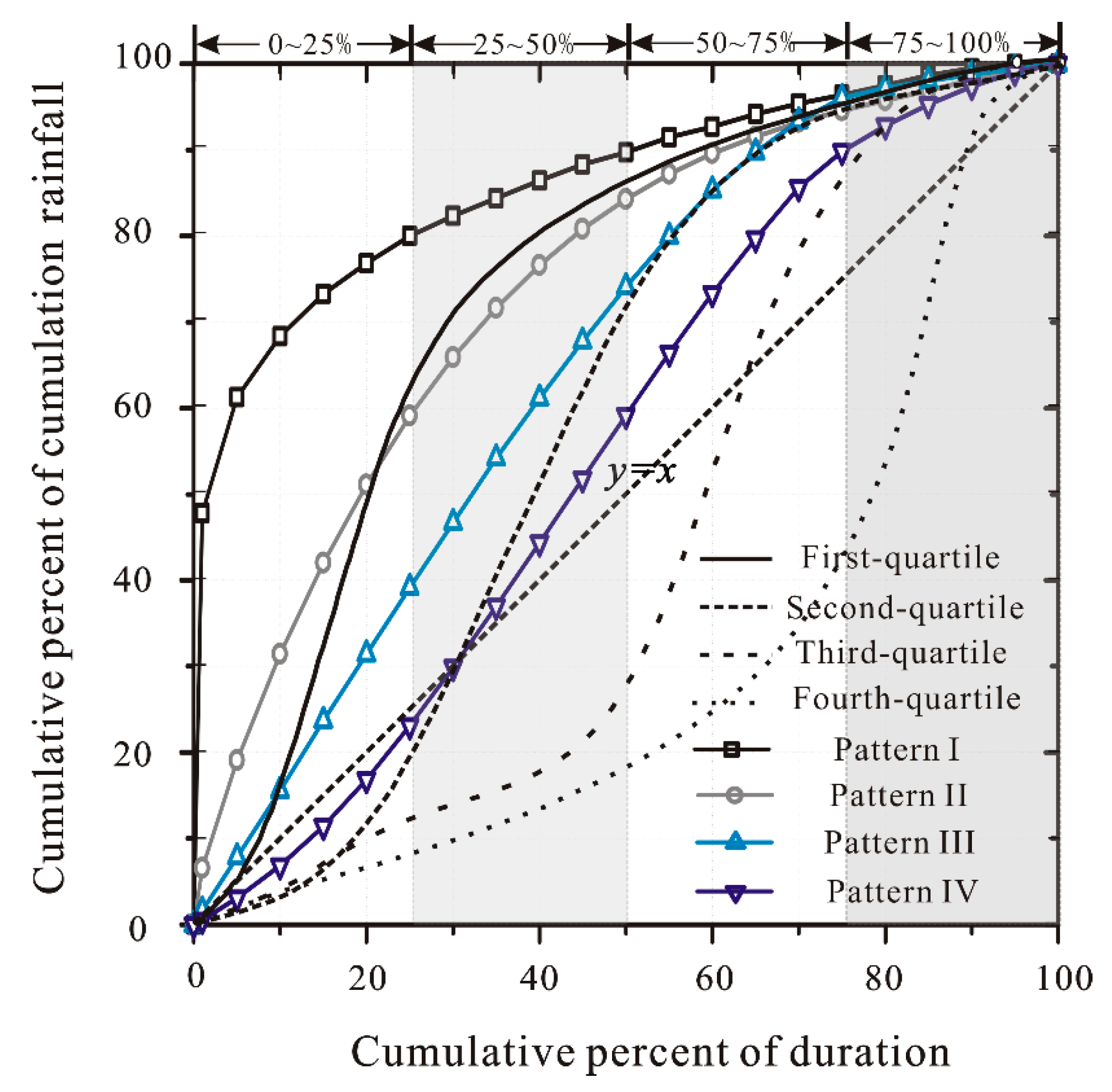
Figure 7 indicates that the period during which the cumulative rainfall increased fastest was in the first period from 0% to 25% of the rainfall duration for Pattern I and Pattern II. These periods were defined as first-quartile rainfall according to the Huff curve. Considering the fact that in most cases, debris flows broke out in the middle and later periods of heavy rain events, Pattern III, with durations from 0–50% of the total duration, was regarded as the second-quartile rainfall; Pattern IV was classified into the same category as Pattern III because the rainfall was concentrated in the duration period of 25–50%.
Through statistical analyses on the rainfall data in the study over the years, the first-quartile and second-quartile rainfalls of Patterns I, II, III, and IV were applied to Xiongmao Gully in order to reveal the hydrological response characteristics under typical rainfall conditions.
As mentioned above, the rainfall intensities within 24 h at frequencies of 1%, 2%, 5%, and 10% in Xiongmao Gully were 211.5 mm, 190.8 mm, 162.0 mm, and 139.5 mm, respectively. The cumulative rainfall curves of Pattern I, Pattern II, Pattern III, and Pattern IV tended towards y = x graph gradually in
Figure 7, and the rainfall intensity concentration degree decreased successively. The typical equations of four cluster centers for the accumulated rainfall (R
a) vs. duration (t) for four types of rainfall pattern were acquired by K-value clustering analysis:
Pattern I, Ra = 0.1219ln(t) + 0.9879, R2 = 0.9815
Pattern II, Ra = 1.7402t3 − 3.984t2 + 3.2591t, R2 = 0.9978
Pattern III, Ra = −0.7667t3 + 0.1624t2 + 1.5868t, R2 = 0.9996
Pattern IV, Ra = −1.8049t3 + 2.3173t2 + 0.4719t, R2 = 0.9997
4.2. Runoff Discharge for Various Rainfall Patterns and Frequencies
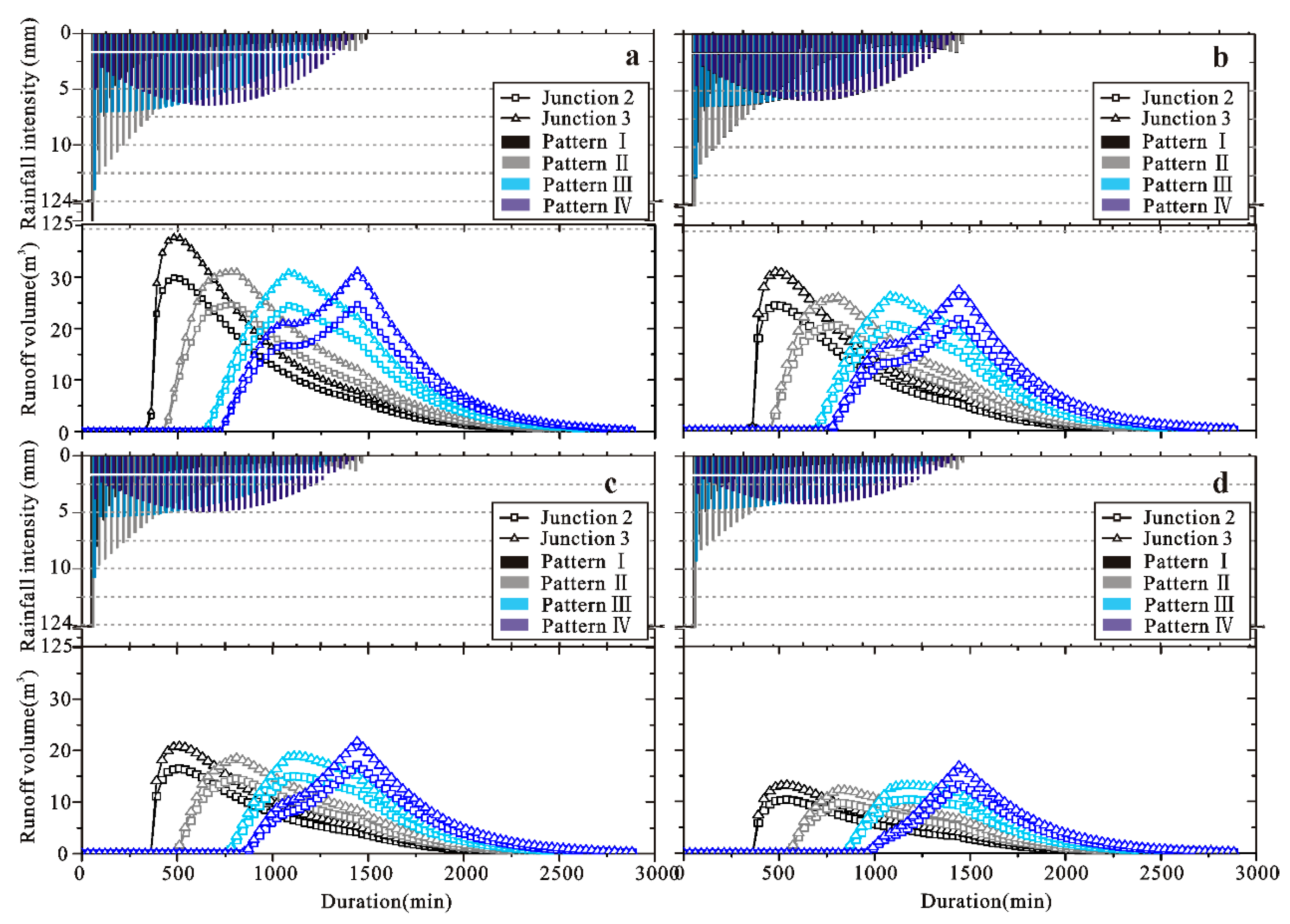
The rainfall intensity at any period could be calculated according to the above equations. The precipitation for a certain period and the distribution diagram of hourly rainfall intensity are presented in the upper part of
Figure 8 for varying recurrent periods. Additionally, the hourly rainfall intensity distributions for different rainfall patterns are distinguished by different colors, corresponding to the discharge hydrograph of the confluence of Junction 2 and 3 in
Figure 6. To present the whole discharge process of a valid rainfall event, the time period was set at 48 h.
Compared to the water volume curve in Xiongmao Gully, the lower part of
Figure 8 shows hydrographs at different junctions for different rainfall return periods and rainfall patterns. The rainfall frequencies influenced the flow volumes, and it was found that the peak discharge was influenced by the rainfall patterns. The time at which the peak flows of Pattern I, II, III, and IV emerged were after 480~510 min, 780~810 min, 1080~1110 min, and 1410~1470 min, respectively. However, as shown in
Figure 8d, the peak flow for a frequency of 10% appeared a little later and lasted for a longer time, indicating that the storage capacity of the vegetation and soil in the catchment retarded and decreased the peak flow.
Pattern I showed larger peak flows at rainfall frequencies of 1% and 2%, because the high intensity rains for this pattern caused high runoff. The peak flows of Pattern I at the rainfall frequencies of 5% and 10% were more or less equal to the peaks of other patterns at the same frequencies, or even less than the runoff peaks of Pattern IV, meaning that larger peaks were more likely to appear in uniform rainfall patterns.
4.3. Discharge of Debris Flow and Threshold on 26 July
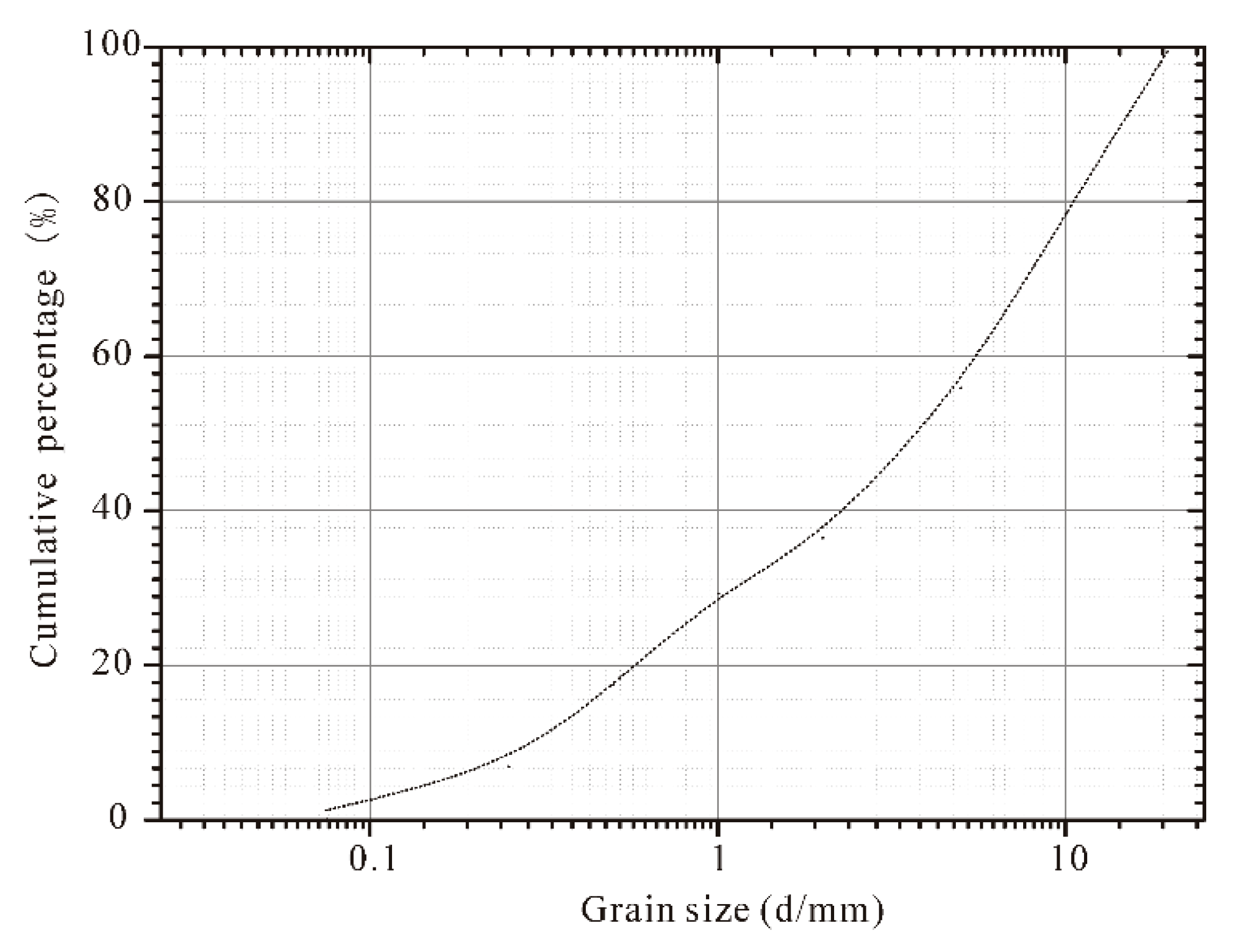
Samples were taken from debris flow deposits and colluvial material at a depth of 0–50 cm for the particle grading test; a grading curve was then acquired from laboratory analyses and grading was done for particle samples smaller than 2 mm (
Figure 9).
The investigated section of the debris flow in Xiongmao Gully, B-B’, was d10 = 0.45 mm, d16 = 0.8 mm, d30 = 1.24 mm, d60 = 18 mm, d84 = 36 mm, tanθ = 0.063; the critical unit discharge of B-B’ was qc = 1.206 m3/s·m, and the critical discharge was Qc = 43.8 m3/s.
Referring to
Figure 9, the granular size Test 4, P
0.05 and P
2 listed in
Table 2, were calculated by Equations (2) and (3); the debris flow density was γ = 1.67 × 10
3 kg/m
3, the volumetric concentration of the solids C
V = 0.42. The field survey indicated that the maximum flow of debris flow on 26 July 2016 was
Qc = 66.7 m
3/s.
Table 2 shows the results calculated from
Figure 9 and Equation (3).
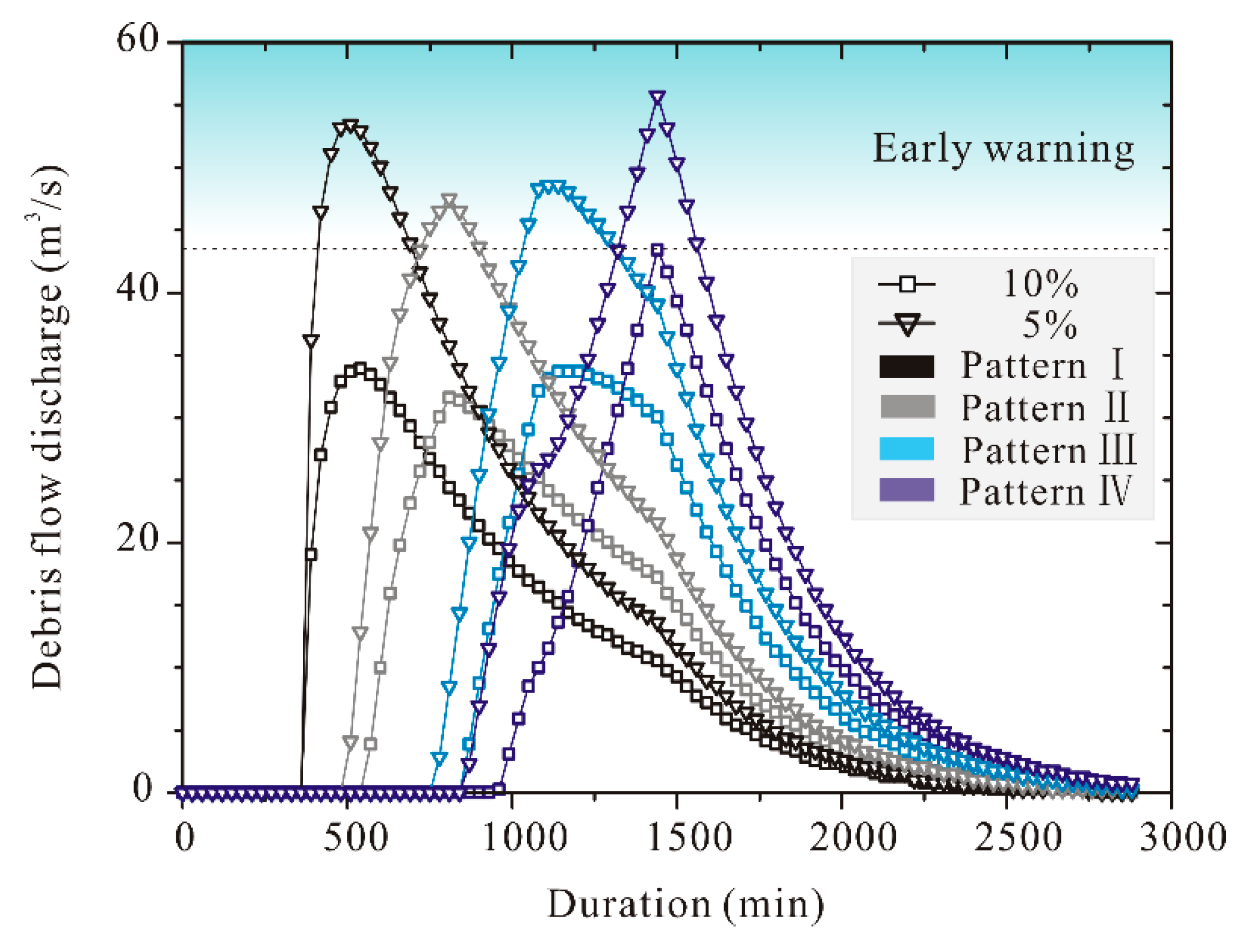
As indicated in the critical discharge analysis, the rainfall conditions led to the outbreak of a debris flow on 26 July 2016; except for the catchment topography and source distribution, the prediction of the rainfall conditions under which debris flow could happen was the aim of this study. The debris flow discharges at cross-section B-B’ under rainfall conditions at frequencies of 10% and 5%, calculated using Equations (1) and (2), are shown in
Figure 10, and it can be seen that debris flow was almost impossible in Xiongmao Gully at the frequency of 10%, while debris flow was more likely under the four rainfall patterns at the frequency of 5%.
The horizontal dotted line in
Figure 10 was the critical discharge at B-B’ corresponding to Junctions 2 and 3, showing four possible rainfall patterns leading to debris flow at the B-B’ cross-section and that critical precipitation and duration varied for different rainfall patterns. The rainfall threshold was maximum in 1h and 6h for Pattern I, and it was the lowest for Pattern IV.
5. Discussion
As shown in
Figure 10, the peak discharge and time were affected by various rainfall patterns and frequencies. In addition, the input parameters in HEC-HMS had great influence on the simulated response, so the sensitivity analysis should be taken into consideration. Some confusion emerged on the debris flow discharge based on Equation (1), due to the uncertainty of D
c value in particular. The main topics discussed herein in terms of debris flow discharge include rainfall patterns, parameters, and uncertain values.
5.1. Statistical Rainfall Patterns
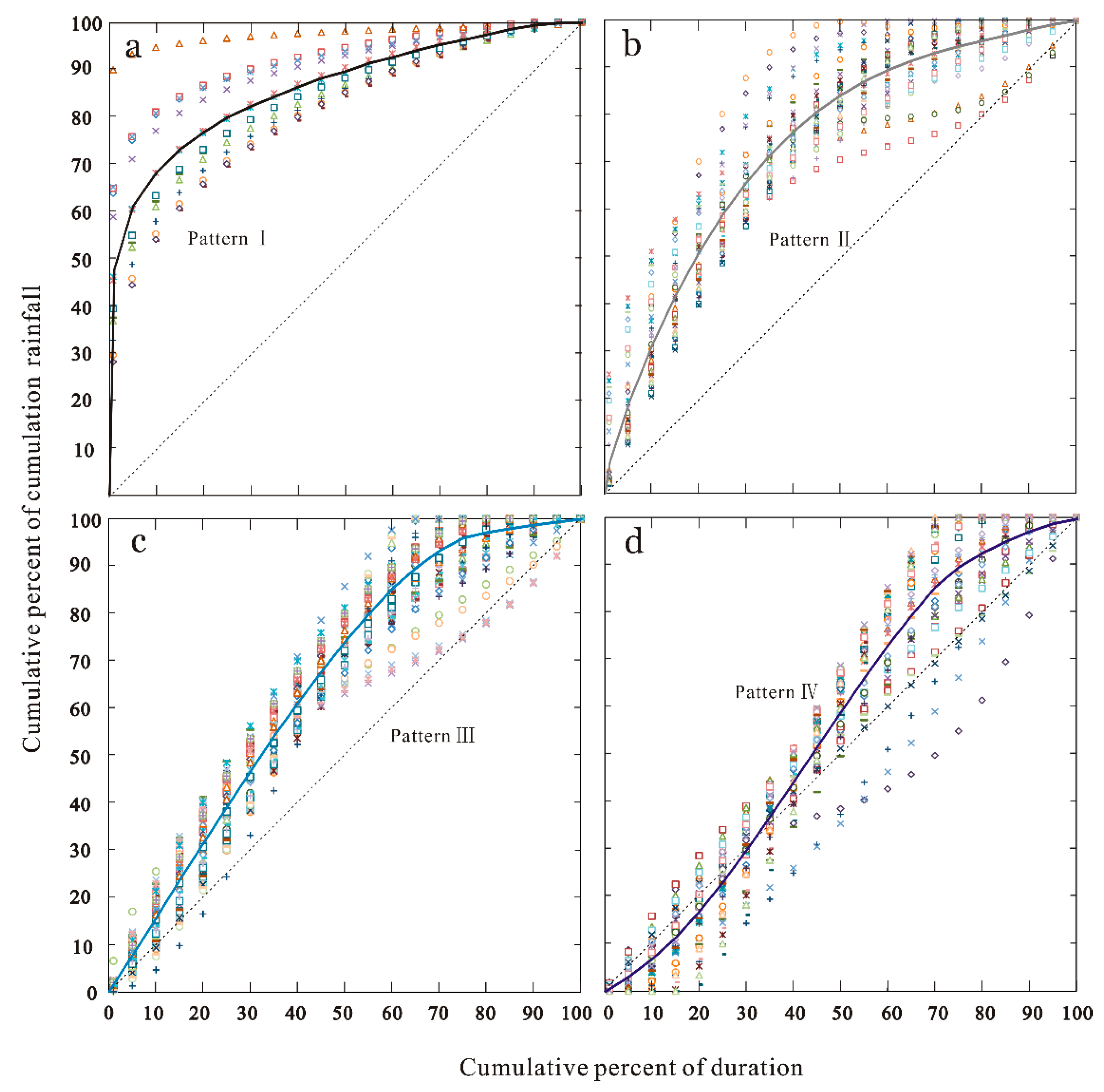
Huff (1967) [
24] divided the curve into first-quartile, second-quartile, third-quartile, and fourth-quartile, and, further, a dimensionless curve was depicted by dividing it into nine probability levels from 10%, 20%, through to 90%. According to the above listed rainfall data and K-value clustering analysis, four patterns, cumulative percentage–duration percentage, were categorized as shown in
Figure 11. Most studies used the median curve as the typical curve, and 50% probability level was the most suitable level for the simulation of runoff discharge in practice.
Figure 11 depicts the Huff curve at a 50% probability level, stressed by the varying dot/dash lines.
For all of the 165 rainfall events, 14 events belonged to Pattern I (8.48%), 40 events to Pattern II (24.24%), 71 events were Pattern III (43.03%), and the rest were Pattern IV (24.24%). The antecedent precipitation dominated in Pattern I. The research results revealed that Pattern I tended towards a temporal rainfall duration of less than 12 h in general. Pattern II represented rainstorms of temporal rainfall as well.
Zhou et al. (2014) [
21] pointed out that the rainfall thresholds varied in the range of 7.8~38.4 mm/h for debris flows which occurred in the Wenchuan earthquake area. For many rainfall events, different rainfall patterns resulted in various discharges and initial water content. Compared with
Table 3, the rainfall threshold of the critical discharge of debris flow varied with rainfall patterns, and the maximum hourly rainfall intensities of Pattern II, Pattern III, and Pattern IV at earlier stage were consistent with the results of the pre-study, while the maximum hourly rainfall intensity was 97.3 mm/h for Pattern I, the abrupt heavy rain mode. It was shown from the maximum rainfall threshold at earlier stage of 1 h and 6 h that antecedent precipitation made the threshold value decrease compared to heavy rainfall of a short duration (Pattern I).
5.2. Parameter Sensitivity Analysis of HEC-HMS
For the hydrograph discharge, sampling tests ensured the accuracy of values such as initial storage, maximum surface storage, and CN values, geographical and climatic factors, potential maximum retention, and maximum vegetation interception proposed in the literature [
34,
36,
38,
45]. Based on the method of sensitivity analysis [
13], the sensitivity of HEC-HMS simulated flow discharge with four parameters, as presented in
Table 4.
With the increasing/decreasing parameters from the simulations, the results were simulated as different percentages of discharge relative to the base case, revealing that CN values plus 10% or minus 10% led to a 28% increase and 16% decrease of peak discharge, respectively. The valuing of CN had a significant influence on flow discharge, while other parameters had a weak influence in Xiongmao Gully.
5.3. Debris Flow Discharge
For the debris flow discharge, Q
p and C
v were based on particle size and specific weight of debris flow or water, and Equation (1) was selected to avoid more parameters beyond D
c. D
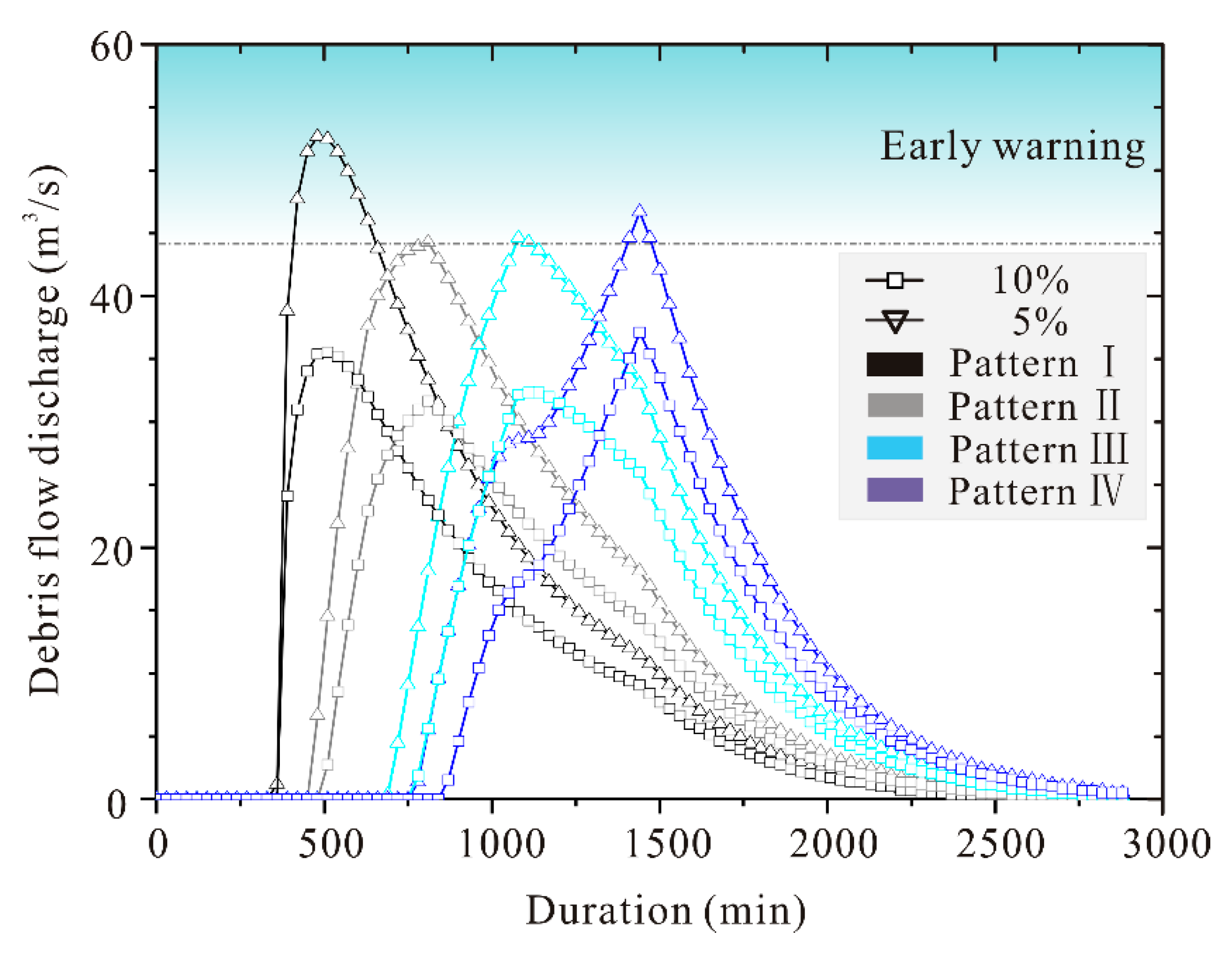
c, valued with the blocking degree of channel, affected discharge significantly. The lowest early warning area when channel blocking (while D
c = 1.0) was neglected is shown in
Figure 12. Compared with
Figure 10 (D
c = 1.5), considering the slight blocking, C-C’ was selected as the analytic crossing section for observable initiation, which could reduce influence on the prediction results for various D
c values. All the patterns at 2% rainfall frequency led to sediment initiation, while discharge may increase along the channel in reality. At the frequency of 5%, shorter durations at 2% frequency generated larger runoff in the Xiongmao catchment.
6. Conclusions
It was indicated by field survey that the 2016 outbreak of debris flow in Xiongmao Gully was due to rainfall runoff flooding and erosion of earlier alluvial deposits along the channel banks and bed. Laboratory test relations were used to calculate the debris flow discharge on 26 July 2016, which was lower than the discharge recorded in the field survey. Based on the analyses presented above, the following conclusions were drawn.
Increasing concentrations of runoff and abundant channel sediment incurred debris flow. The gentle gradient and straight channel upstream and midstream ensured that debris flow on Xiongmao Gully developed slightly with increasing concentration and discharge. With a return period of 2%, deposition was initiated primarily in the wide middle of the stream.
The critical discharge at the B-B’ cross-section was 43.8 m3/s, lower than that recorded in the morphological survey on the critical discharge of debris flow Qc = 66.7 m3/s (at the frequency of 2%).
K-value clustering analysis of the precipitation revealed that there were four rainfall patterns. Pattern I and Pattern II represented cumulative rainfall growing fastest in the duration from 0% to 25%, characterized by heavy rainfall with short duration, which accounted for 32.7% of events; the duration period in which rainfall was concentrated most was in the range of 25~50% for Pattern III and Pattern IV, in proportion of 67.3%.
Debris flow was more likely to occur under four rainfall patterns at the frequency of 5% in Xiongmao Gully; however, with the debris material decreasing upstream, a rainfall frequency of 2% would be required.


