Abstract
Numerical modeling is widely acknowledged as a highly precise method for understanding the dynamics of contaminant transport in groundwater. However, due to the intricate characteristics of environmental systems and the lack of accurate information, the results are susceptible to a significant degree of uncertainty. Numerical models must explicitly consider related uncertainties in parameters to facilitate robust decision-making. In a Chromium Residue Site located in southern China (the study area), this study employed Monte Carlo simulation to assess the impact of variability in key parameters uncertainty on the simulation outcomes. Variogram analysis of response surface (VARS), global sensitivity analysis, and an XGBoost (version 2.0.0)-based surrogate model was employed to overcome the substantial computational cost of Monte Carlo simulation. The results of numerical simulation indicate that the contaminant is spreading downstream towards the northern boundary of contaminated site near Lianshui River, threatening water quality. Furthermore, migration patterns are complex due to both downstream convection and upstream diffusion. Sensitivity analysis identified hydraulic conductivity, recharge rate, and porosity as the most influential model parameters, selected as key parameters. Moreover, uncertainty analysis indicated that the variability in key parameters has a minimal impact on the simulation outcomes at monitoring wells near the contaminant source. In contrast, at wells positioned a considerable distance from the contaminant source, the variability in key parameters significantly influences the simulation outcomes. The surrogate model markedly mitigated computational workload and calculation time, while demonstrating superior precision and effectively capture the non-linear correlations between input and output of the simulation model.
1. Introduction
Transport of contaminants through groundwater presents substantial environmental concerns, resulting in the degradation of freshwater reservoirs and a decline in drinking water standards. The quantity and quality of freshwater play pivotal roles in shaping the surrounding ecosystem, notably affecting aquifer integrity [1]. Contaminants commonly consist of heightened concentrations of substances like heavy metals and toxins, posing threats to water reservoirs [2]. The rapid industrialization in China has served as a catalyst for socioeconomic advancement; however, at same time, it has led to the contamination of groundwater environments with heavy metals [3]. The transport of heavy metals contaminants in groundwater is an imperceptible, prolonged, challenging-to-detect, and reversible phenomenon [4]. Among them, Chromium (Cr) groundwater contamination often stems from the unregulated disposal of chromium slag and the seepage of leachate from slag piles. Chromium (Cr) is typically present in trivalent (Cr(III)) and hexavalent (Cr(VI)) states [5], in which Cr(VI) poses a significant environmental concern, adversely affecting the ecosystems and water quality [6,7]. Due to its high toxicity [8], mobility, and dissolvability [9], it poses substantial threats to the prospects of sustainable development [10,11]. Having recognized the hazardous nature of Cr, the United States Environmental Protection Agency (US EPA) added it to the priority pollutant list. Therefore, a comprehensive understanding of the dynamic features governing Cr(VI) contaminant transport is crucial for accurate contamination assessment, and effective remediation, contributing to the overall goal of sustainable development.
With advances in computational techniques, numerical simulation of contaminants in ground waters has become a predominant approach for studying contaminants behavior in groundwater systems [12,13]. In recent years, several numerical simulations of groundwater investigations have been conducted to simulate the transport of Cr(VI) contaminant [10,14,15,16,17].
The hydrodynamic processes governing the flow of groundwater and the transportation of contaminants in an aquifer are a very complex, introducing numerous uncertainties in the numerical modeling outcomes. These uncertainties encompass aspects related to model parameters [18], the conceptual model [19,20], and observational data and measurements [21,22]. Accurate data for groundwater simulation model parameters are hindered by high testing costs, measurement errors from non-calibrated devices, and the complex behavior of water movement in aquifers. Consequently, providing precise values for simulation parameters is impractical, necessitating the incorporation of a reasonable level of uncertainty [23]. Input parameter inaccuracies can further impact model outputs, stemming from measurement error [24]. To enhance model reliability, it is crucial to perform uncertainty analyses on simulation model parameters to reduce the possible risk in the failure of model [25].
In parameter uncertainty analysis, the preeminent methodologies employed with highest frequency encompass sensitivity analysis and the Monte Carlo method [26]. Sensitivity analysis serves as an essential evaluation technique, providing valuable understanding into how variations in input factors, such as model parameters, affect model responses [27]. Sensitivity analysis comprises two main approaches: Local and Global sensitivity analysis [28]. Local sensitivity analysis focuses on model sensitivity within a specific parameter range, while global sensitivity analysis examines sensitivity across the entire parameter spectrum [29]. Methods for local sensitivity analysis include the one-factor-at-a-time technique [30] and regional sensitivity analysis [31]. Global sensitivity analysis employs various approaches, including the derivative-based [32], variance-based [33], and the recently developed Variogram Analysis of Response Surfaces (VARS) architecture [34,35]. While the ultimate aim of uncertainty analysis is to explore the full range of potential outcomes and their associated probabilities, sensitivity analysis only assesses the impact of input variations on output values [36].
The Monte Carlo method is a commonly employed technique for evaluating model uncertainty [37]. Monte Carlo simulation proves to be a versatile and straightforward technique capable of translating the uncertainty associated with model parameters into corresponding uncertainties in simulation outcomes, making it well-suited for assessing uncertainties in multivariable models [38]. In the context of uncertainty analysis, Monte Carlo method necessitates running the numerical model multiple times, leading to significant time consumption, especially when dealing with a complex model directly invoked. The surrogate model serves as an approximation of the simulation model, mitigating computational burdens and reducing processing time without compromising accuracy [39]. The surrogate model emulates the functionality of the simulation model and attempts to approximate the inherent association between groundwater parameters and contaminants distribution, all accomplished with a minimal computational load [40].
In recent years, several surrogate model approaches have been suggested to approximate simulation models for uncertainty analysis, such as Polynomial Chaos Expansion (PCE); Gaussian Process Emulation (GPE) [41]; Gaussian processes [42]; Kriging [26,43,44]; Radial Basis Function (RBF) [45]; Support Vector Regression (SVR) [46]; Artificial Neural Network (ANN) [47]; Multi-gene Genetic programming (MGGP) [48]; Kernel Extreme Learning Machine (KELM) [49]; a hybrid approach using the Multilevel Monte Carlo method (MLMC); a graph convolutional neural network and a feed-forward neural network [50]; and a Deep Belief Neural Network (DBNN) [51]. While earlier studies have demonstrated certain achievements, the application of surrogate models encounters challenges related to scalability and accuracy, particularly in scenarios where contaminant-related associations exhibits pronounced non-linearity or high dimensionality [52]. Ensemble learning surrogate models integrate various surrogate models to generate a comprehensive prediction, allowing for the compensation of errors from individual surrogates by utilizing the collective knowledge of the ensemble [53]. Extreme Gradient Boosting (XGBoost) is an illustrative ensemble learning model that integrates the predictive results of individual decision trees to address regression tasks, demonstrating significant potential in the domain of surrogate modeling [54]. However, the significantly increasing computational costs due to the introduction of multiple surrogate models is the major concerns in applying ensemble learning surrogate models to groundwater contaminant transport modeling. Additionally, there has been limited attention in existing research on global sensitivity analysis, primarily focusing on local sensitivity analysis methods. This limits valuable understanding into how variations in input model parameters affect model responses.
Our study presents a novel and robust Variogram-based Global Sensitivity Analysis (VARS) to identify the most influencing parameters on the model output, as key parameters. Additionally, we proposed an XGBoost surrogate model to reduce the computational cost of Monte Carlo simulation. The Monte Carlo simulation was employed to assess the impact of variability in key parameters uncertainty on the results of groundwater contaminant transport model. The Chromium Residue Site located in southern China was chosen as the study area. This research addresses the following challenges: (1) Application of numerical modeling to simulate and analyze the behavior of contaminated site in the context of groundwater contaminant transport; (2) VARS sensitivity analysis to comprehensively assess the impact of input parameter variations on model outputs; and (3) Uncertainty analysis utilizing the proposed XGBoost surrogate model to approximate the outcomes of the groundwater contaminant transport model, facilitating a more computationally efficient analysis of parameter uncertainties.
2. Materials and Methods
2.1. Overview of Study Area
This paper examines a chromium-contaminated urban site that was previously operational ferroalloy refinery, situated in a South China as illustrated in Figure 1. The plant was constructed in 1958, officially started production in 1962, shutdown all factory operation in 2006, and it was completely dismantled in 2010. The Ferroalloy plant, occupying an area of around 590,141 m2, primarily produced metal chromium, carbon-manganese and pig iron. The production process involved utilization of raw materials such as silicon, manganese, chromium, and iron. The ferroalloy plant, situated in close proximity to Lianshui river, consistently produced chromium metals for over five decades, resulting in a substantial accumulation of chromium-bearing slags and tailings during this historical timeframe. Improper storage in open yard near the plant has led to leachate from rainfall induced slag infiltration, causing soil and groundwater pollution.
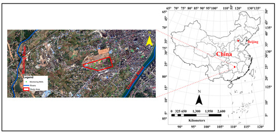
Figure 1.
Location of study area.
Based on geological drilling data obtained from the geological investigation, the region is characterized by a heterogeneous composition, including miscellaneous fill, silty clay, medium sandsilt-round gravel, weathered mudstone, and moderately weathered mudstone. The miscellaneous fill exhibits high porosity, contrasting with the aquiclude nature of the silty clay layer, which has limited water permeability. The primary confined aquifer is represented by the medium sandsilt-round gravel layer, featuring moderate porosity, while the less permeable mudstone layer forms the base.
A technical roadmap of the proposed methodology is illustrated in Figure 2. A conceptual model was developed from the conversion of the 3D geological model pre-processes to match the input format for the Groundwater Modeling System (GMS). Numerical model of Cr(VI) contaminant transport constructed in groundwater for analyzing the spatial and temporal changes of Cr(VI) contaminant, based on calibrated groundwater flow model. However, in numerical models, the presence of uncertainty associated with hydrogeological parameters is frequently inherent, challenging to ascertain, and contributes to uncertainty in the outcomes. Therefore, the VARS sensitivity analysis method was employed to determine the highly sensitive parameters within the system, subsequently utilized as the key input parameters. Latin hypercube sampling was applied within the probability distribution and range of values of key parameters to generate the input datasets. Then, a groundwater Cr(VI) contaminant transport numerical model was used to generate input–output dataset. An XGBoost surrogate model of groundwater Cr(VI) contaminant transport numerical model was established according to the input–output dataset. The surrogate model was built to reduce the computational burden caused by frequent invoking of the simulation model, thereby enhancing overall computational efficiency. Based on the surrogate model, the Monte Carlo simulation was used to evaluate the uncertainty caused by variability in key parameters and their impact on the output of numerical model.
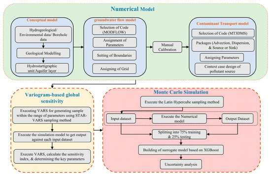
Figure 2.
Technical roadmap of proposed methodology.
2.2. Numerical Modeling
Numerical modeling is a robust tool for assessing, simulating, and predicting the movement of contaminants in groundwater flow systems. This process involves the following steps [10]: (1) development of conceptual model, (2) development and calibration of groundwater flow simulation model, and (3) Cr(VI) contaminant transport simulation model.
In this paper, the simulation of groundwater flow and contaminant transport was conducted using the MODFLOW-2005 and MT3DMS modules integrated within the Groundwater Modeling System (GMS) software (version 10.6) [55]. A calibrated MODFLOW model was utilized for the MT3DMS model. Furthermore, to acquire a comprehensive insight of Cr(VI) transportation during the simulation and for further studies, eight monitoring wells were used to observe the Cr(VI) transportation (Figure 3).
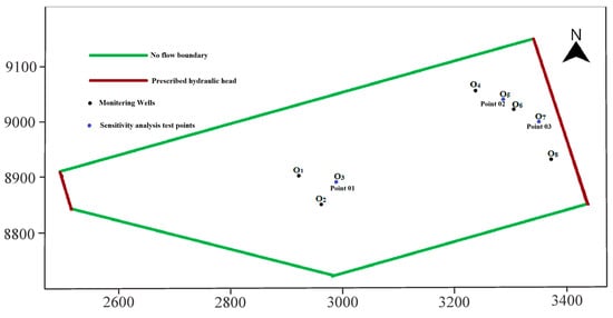
Figure 3.
The boundary of study area, distribution of monitoring wells, and locations of sensitivity analysis test points.
2.2.1. Conceptual Model
Previous studies [56,57] confirm the practicality of extracting hydrogeological model surfaces from GOCAD software (version 2017) geological model in either TIN or ASCII format for integration into Visual MODFLOW or GMS. A three-dimensional model of the study area (Figure 4) developed through a systematic process: (1) construction of a geological model using GOCAD’s structural and stratigraphic workflow, incorporating data from 30 boreholes, (2) preservation of corrected strata in ‘ASCII’ point files, and (3) application of the Inverse Distance Weighting (IDW) method in GMS for the interpolation of ‘ASCII’ point files. For conceptual model development, a finite-difference grid has been employed as a solving framework. The study area is discretized and modeled into finite difference cell-centered grid of 100 rows and 90 columns, ensuring that each cell maintains a size of 5 m (Figure 4). The modeled domain consisted of 45,000 cells, of which 22,325 were active cells and 22,675 were inactive cells.
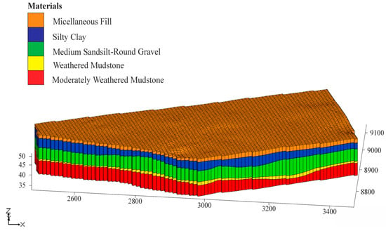
Figure 4.
3D finite difference cell centered grid of study area.
In the numeric simulation, we exclusively focused on sandsilt-round gravel layer. This layer contains the confined pore water and is treated as the confined aquifer. Other layers, at the top and bottom of the sandsilt-round gravel layer, are characterized by low permeability and are regarded as unconfined aquicludes. Taking into account that there is no natural boundary at the study area, the study area was defined by the Wuming and Lianshui Rivers in the northwest and southeast, respectively, serving as the constant head boundaries in their respective regions (Figure 3). As the aquifer possessed a specific depth of embedment, the impact of evaporation was disregarded [14]. Groundwater in the area mainly receives recharge from rainfall and surface water, and the flow direction is from northwest to southeast to the Lianshui River. According to the hydrological survey for the site, the head is 51 m at northwest and 47 m at southeast boundaries.
2.2.2. Numerical Simulation Model
Groundwater flow models determine hydraulic heads and thereby velocities within an aquifer. This information is then incorporated into a transport model to simulate the migration of contaminants carried by the groundwater [58]. Governing partial differential equation for three-dimensional groundwater flow in saturated porous media is based on Darcy’s Law can be written as Ref. [59]:
where, , , denote the hydraulic conductivities in , , and dimensions, respectively; denotes the hydraulic head; represents the sink/source; is coefficient of specific storage, and represents the time.
A contaminant transport model serves as a simplified representation of geochemical conceptual model, focusing on the predicting the concentration of a dissolved chemical, such as Cr(VI), in an aquifer at a given location and time. This simplification is achieved through dynamics equation describing convection-dispersion of contaminant transport in three dimensions, including internal sources or sinks, can be written as [60]:
where is the dispersion coefficient, is the Darcy speed, is concentration, denotes effective porosity, represents source or sink concentration, and represents the source or sink flow rate per unit volume.
We use the dynamic models formulated in Equations (1) and (2) to simulate the groundwater contaminant transport process. The dynamic model was solved using GMS software (version 10.6). During the simulation, boundary conditions outlined in Figure 3 were applied, and the initial concentration for contaminant transportation was determined based on the concentrations measured in 2017, as described in Figure 5 [61]. Additionally, a constant concentration of 120 mg/L was hypothetically applied to the contaminant sources based on the observations from wells in close proximity to these sources. No adsorption processes were assumed in the model for Cr(VI) contaminant transport, and thus, the Cr(VI) can be considered as a conservative specie. The contaminant transport model was simulated over the period from 2017 to 2020. All parameters, including the calibrated hydraulic conductivity, as well as other parameter values of the confined aquifer (i.e., medium sandsilt-round gravel layer) input to the numeric simulation, along with their respective reasonable ranges [49], have been summarized in Table 1.
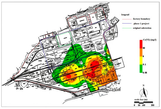
Figure 5.
Initial contaminant concentration in groundwater [61].

Table 1.
Values and ranges of parameters of medium sandsilt-round gravel confined aquifer.
2.3. Variogram-Based Global Sensitivity Analysis (VARS)
In 2016, Razavi and Gupta [34,35] proposed a novel approach for a global sensitivity analysis called Variogram Analysis of Response Surfaces (VARS), which builds upon the Variogram concept. Variograms prove to be robust tools for describing the spatial or spatiotemporal framework and variance of a target variable, such as a model response across various perturbation scales in multi-parametric space [62]. Through the modeling of spatial variation in the variogram, VARS establishes the two types of global sensitivity approaches (GSA), variance-based [33] and derivative-based [32], making it significantly efficient than these two most widely-used GSA methods, while still producing nearly consistent results [34,35]. In addition, compared to other popular techniques like Morris [32] or Sobol [33], VARS offers much more efficient GSA with a considerably lower number of model evaluations [63].
VARS analysis characterizes the spatial variance and interrelation of the model output within a domain delineated by a set of various parameters. Let’s consider a scenario where the model output, , this is a function dependent on parameters . Let denote the position within the -dimensional parameter space. be the distance vector between any two points in the parameter space. The multidimensional variogram can be computed under intrinsic stationary assumptions as:
When the variogram is computed along dimension (parameter), such that for all , the resulting variogram is one dimensional, known as a directional. Directional variograms focus on the distance between pairs of points along specific parameter directions rather than their locations in the parameter space.
Directional variograms serve as the foundational elements of VARS and describe the sensitivity of model output to each parameter across a comprehensive range of perturbation scales, denoted by . Integrated Variogram Across a Range of Scales (IVARS), a unique sensitivity index can be calculated by integration of variograms for the parameter up to a designated perturbation scale of concern (e.g., 10%, 30% or 50% of the parameter range):
The value indicates how the sensitive of model output is to parameter at any specific ranges . IVARS50 ( of the parameter range) is known as total variogram effect and can be regarded as the most inclusive index within the VARS structure to evaluating global sensitivity of a response surface to each respective parameter.
A novel and robust “star-based” sampling approach, denoted as STAR-VARS has been developed for the VARS numerically implementation, enhancing computational efficiency [35]. First, a sampling technique such as the Latin Hypercube or Progressive Latin Hypercube [64] is used to choose N star centers from the parameter space. Next, equidistant points, or ‘stars,’ are created along each parameter dimension for each star center. These stars are employed in computing sensitivity metrices like IVARS, based on a defined resolution (). The total number of sample (computational cost) associated with implementation of STAR-VARS is calculated using Equation (5).
where and represent the number of star centers, respectively, the number of input parameters, and perturbation resolution (that is minimum space between pairs of point within the parameter space).
In our study, we utilized a comprehensive version of the recently developed VARS-tool package in Python to implement the STAR-VARS. Our experimental setup of VARS involves following steps:
- (1)
- The parameters listed in Table 1 were selected for sensitivity analysis. A ±20% variation range was set for each sensitive parameter.
- (2)
- A total 300 random sample points are created by employing a star-based sampling method within defined parameter ranges. The sampling attributes utilized in STAR-VARS are detailed in Table 2.
- (3)
- Generated random sample points were input into the numeric simulation model. The numeric simulation model outputs concentrations of the Cr(VI) contaminant at three test points. The locations of three test points are illustrated in Figure 3.
- (4)
- The output concentrations of the Cr(VI) contaminant were then processed further in the VARS model. Specifically, the IVARS-50 index was executed to calculate a set of sensitivity indices for each test point.

Table 2.
Sampling attributes for STAR-VARS.
Table 2.
Sampling attributes for STAR-VARS.
| Number of Stars | ) | Perturbation Resolution | Sampler | Bootstrap Size | Confidence Interval (%) |
|---|---|---|---|---|---|
| 5 | 0.1 | 0.1, 0.3, 0.5 | Latin Hypercube | 1000 | 90 |
2.4. Surrogate Model Based on Extreme Gradient Boosting
Chen and Guestrin [65] introduced Extreme Gradient Boosting (XGBoost) in 2016 as an advanced ensemble learning algorithm within the boosting framework. Its foundation in decision tree methodology enhances predictive modeling capabilities. Boosting algorithms construct base estimators to correct errors, fostering strong interdependence. In contrast, bagging creates independent base estimators for diversity. The strong correlation in boosting reflects cooperative model improvement [65]. Unlike the gradient boosting structure, XGBoost regularizes the loss function within the objective function. This regularization contributes to smoother learning weights and reduces the risk of overfitting [66]. XGBoost algorithm iteratively refines the model’s structure and parameters using an objective function, contributing to enhanced predictive accuracy [67].
This approach uses an ensemble of trees to predict the results, relying on total number of trees in the ensemble denoted as , where denotes the feature values associated with sample , and signifies the actual value of the sample for prediction; is the space of trees in the ensemble. The final prediction for a given sample is determined by the cumulative sum of predictions generated by each individual tree, expressed mathematically:
Within provided dataset, corresponds to an independent tree. The leaf weights represent the values associated with each leaf node in the regression trees, where and is the entire number of leaves on the tree. The objective function can be specifically described as:
where denotes the loss function which measure the difference between predicted and actual values; is total number of samples in dataset used to train or evaluate the model. Gamma and lambda in the objective function contribute to the regularization of model, with controlling the tree structure and penalizing the magnitude of the weights. The regularization terms () prevent models from becoming overly complex and fitting the training data too precisely, thereby enhancing the model’s ability to generalize well to new, unseen data and avoiding overfitting.
In the training phase of XGBoost, the construction of tree structures occurs in a sequentially. The creation of a new tree is influenced by the predictive outcome of the preceding tree, leading to adjustments in the residuals within the predicted values. The Equation (8) defines optimum weight for a specific leaf in a fixed tree structure.
where terms are the first and second-order derivatives of the loss function during the iteration. With determined optimum leaf weight , the optimal objective function can be formulated as:
The Surrogate model is a black box which effectively captures the non-linear correlations between input and output of the simulation model. The surrogate model reduces computational workload and calculation time. Thus, XGBoost surrogate model is implemented to alleviate the computational burden caused by frequent invoking of the simulation model, thereby enhancing overall computational efficiency. We further developed Random Forest (RF) [68] surrogate model in order to compare the performance of XGBoost surrogate model. Random forest is an ensemble learning method wherein numerous decision trees are constructed with limited interdependencies, which has been used to establish surrogate model for uncertainty analysis in groundwater numerical simulation and has achieved good results [69]. The surrogate model building involves following steps:
- (1)
- Key parameters were selected through VARS sensitivity analysis, treated as stochastic variables to assess the influence of uncertainty related to these parameters on simulation outcomes.
- (2)
- Key parameters were sampled based on their probability distributions and range of values using Latin hypercube sampling (LHS) method [70] to generate 140 input datasets (various combinations of the three key parameters). The values of the remaining model parameters were kept constant with previous adjustments.
- (3)
- These datasets were input into the simulation model. The simulation model was resolved using GMS software to produce corresponding output datasets (Cr(VI) contaminant concentrations observed in 8 monitoring wells), forming Input-output dataset.
- (4)
- Two methods (XGBoost and RF) were employed to build the surrogate model. The input and output datasets were partitioned, allocating 75% for training the model and reserving 25% for validating the accuracy of the surrogate model. This study employed python programming language (version 3.11.5) and the XGBoost library (version 2.0.0), as well as scikit-learn library for Random Forests (version 1.3.0).
- (5)
- To craft optimal surrogate model architectures, hyperparameters were carefully selected to address overfitting during training, thereby enhancing the accuracy of the model (Table 3). The lower and upper values used for these hyperparameter are shown in Table 3. In this study, Optuna Hyperparameter Optimization (OHPO) [71] was employed to automatically fine-tune the hyperparameters of the surrogate model.
 Table 3. Optimized hyperparameters generated by Optuna hyperparameter optimization.
Evaluating the prediction accuracy and efficiency of the surrogate model is essential, as inaccurate models can squander resources and impair optimization, predictions, and feasibility analysis [72]. In this study, the evaluation of surrogate model accuracy in approximating the simulation model involves the use of key metrics, namely the coefficient of determination (R2), mean relative error (MRE), mean-squared error (MSE), and root mean-squared error (RMSE). These metrics, essential for assessing performance, are computed in the following manner:
where represents number of samples, , and denote outcomes of the simulation model and predictions of the surrogate model for the th sample, respectively. is the mean of simulation model results. R² values range from 0 to 1, with 0 indicating that the surrogate model does not explain any variability in the actual values, and 1 indicating the surrogate model explains all the variability in the actual values. A lower MRE, MSE, and RMSE indicate better accuracy, while a higher MRE, MSE, and RMSE suggest larger discrepancies between predicted and actual values. Especially, an MRE of 1 suggests that, on average, the predictions are off by the same magnitude as the actual values. Overall, R² value and MRE can provide a reference of standard metric values for the evaluation of surrogate model. The surrogate model achieves higher accuracy with R² values approaching 1 and smaller MRE, MSE, and RMSE values.
2.5. Monte Carlo Simulation
Based on statistical probability theory, the Monte Carlo simulation is the most widely employed technique for analyzing the uncertainty resulting from complicated mathematical models [73]. The Monte Carlo simulation is characterized by its conceptual simplicity, versatility across various applications, and its unique capability to thoroughly quantify the uncertainties associated with model outputs [74]. Monte Carlo simulation is divided into the following steps [60]:
- (1)
- Determine the random/key parameters by means of sensitivity analysis.
- (2)
- Generation of randomly samples using Latin hypercube sampling method within the feasible region of key parameters.
- (3)
- Run a simulation model for each sample dataset to extract the corresponding model output.
- (4)
- After the completion of all simulations, the construction of a histogram of all simulation results for the uncertain quantity of interest. From the frequency plot, the probability at any level can be estimated. The mean, variance, confidence limit, and other statistical parameters can also be determined.
3. Results and Discussion
We carried out experiments to validate the efficiency of the proposed method. The experiments were conducted on an ordinary PC equipped with an Intel Core i7-6700 processor (3.4 GHz, 8 GB RAM) on a 64-bit Windows 10 system.
3.1. Numerical Simulation of Flow Field and Cr(VI) Contaminant Transport
Figure 6 illustrates the east-to-west flow of groundwater within the study area. Hydraulic head is higher in the northwest and lower in the southeast, by the topography of the area. Groundwater primarily flows laterally towards the Lianshui River, exhibiting a gradual decline in vertical hydraulic gradient. The depth of the groundwater flow is 15 m according to the depth of impermeable based layer (i.e., moderately weathered mudstone) of aquifer. The water head values presented in Figure 6 are indicative of the water table within the aquifer system. The aquifer, in this case, is deemed as having a simple and singular structure [11].
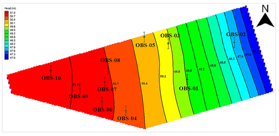
Figure 6.
Groundwater flow patterns in steady state.
Observation data acquired from ten groundwater level monitoring wells in 2019 (Figure 6) was used to calibrate the numeric groundwater model. The results in Figure 7 of the calibration process indicate a high alignment between the simulated and observed hydraulic heads (Figure 7a), with a significant correlation coefficient of 0.973 within the study. Residual analysis indicates a low residual between simulated and observed hydraulic heads, with a mean residual of 0.0023, a mean absolute residual of 0.14, and a root mean squared residual of 0.17. These values fall within allowable range. Figure 7b shows the comparison between simulated and observed hydraulic heads across ten monitoring wells. Both lines exhibit similar trend, indicating that simulation closely matches the observed hydraulic heads. This calibration results shows a good fit between the simulated and observed hydraulic heads.
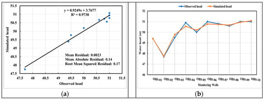
Figure 7.
Results of calibration of hydraulic heads: (a) scatter versus observed and simulated hydraulic heads; (b) comparison of observed and simulated hydraulic head at ten monitoring wells.
The spatial and temporal changes in Cr(VI) over 6, 12, 18, 24, 30, and 36 months are illustrated in Figure 8. As illustrated in Figure 8a–f, the contamination area for Cr(VI) progressively expanded with increasing simulation time under natural conditions. Additionally, the movement of the Cr(VI) contaminant plume consistently followed the direction of groundwater flow. Over the 36-month simulation period, the Cr(VI) pollution plume at the contaminated site continuously spread towards the northern boundary of contaminated site near Lianshui River. Consequently, a lot of attention has been drawn to the water quality. The concentration variation of Cr(VI) in the monitoring wells, presented in Figure 9, illustrates a progressive increase in Cr(VI) contaminant concentration within the groundwater across all monitoring wells (O1 to O8). The concentration curves of each well indicate a consistent rise in Cr(VI) levels over the 36-month period. While the concentration in each well shows a distinct upward pattern, contamination of groundwater near the affected site and downstream areas of the Lianshui River, as highlighted by monitoring wells O3, O5, O6, and O7, posed a significant threat due to elevated levels of Cr(VI).
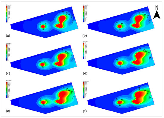
Figure 8.
Transport of Cr(VI) in the study area: (a) 6 months; (b) 12 months; (c) 18 months; (d) 24 months; (e) 30 months; (f) 36 months.
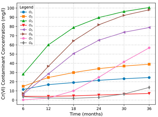
Figure 9.
Concentration changes curve of Cr(VI) in the monitoring wells.
The above results indicate that hexavalent chromium (Cr(VI)) primarily moves downstream due to convection (fluid flow). However, there is also diffusion of Cr(VI) occurring in the upstream direction, creating a more complex migration pattern in the system. In fact, the movement and behavior of hexavalent chromium (Cr(VI)) in groundwater highlight the influence of two factors: hydraulic gradients and concentration gradients [11]. Areas with high gradients of hydraulic heads facilitate rapid downstream movement, while high concentration gradients drive convection from areas of high concentration to areas of low concentration.
As the contaminant plume continuously expands and the area of high concentration regions gradually increases due to the migration of Cr(VI), it is necessary to set remediation facilities, such as pumping wells and permeable reactive barriers (PRBS), in the downstream location of the site to effectively reduce the risk of chromium pollution in the downstream area.
3.2. Sensitivity Analysis
3.2.1. Directional Variograms
Figure 10 presents in the directional variograms of hydraulic conductivity, recharge, and porosity. The results distinctly illustrated that hydraulic conductivity, recharge, and porosity have the most substantial influence on the numeric simulation model output (Cr(VI) contaminant concentrations observed at three testing points at the end of simulation period). Conversely, the remaining parameters exhibit lower sensitivity. Moreover, it is essential to recognize that the sensitivity is influenced by the perturbation scale. Parameters display intricate sensitivity when subjected to a greater magnitude of variations across the perturbation scale, and conversely, sensitivity decreases with smaller magnitude. Parameters characterized by less sensitivity exhibited constrained variability in variograms over the perturbation scale, indicating their comparatively minor influence on the model outputs.
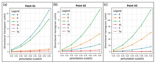
Figure 10.
Directional variogram results of point 01–point 03 (a–c).
3.2.2. Sensitivity Index IVARS-50
The VARS-based most comprehensive sensitivity index IVARS-50, called ‘Total-Variogram Effect’ is selected. The results of analysis are shown in Figure 11. The parameters are ordered by parameter sensitivity. Overall, hydraulic conductivity, recharge, and porosity are the most influential parameters, followed by longitudinal dispersivity. The remaining parameters have minimal effect on the model outputs.
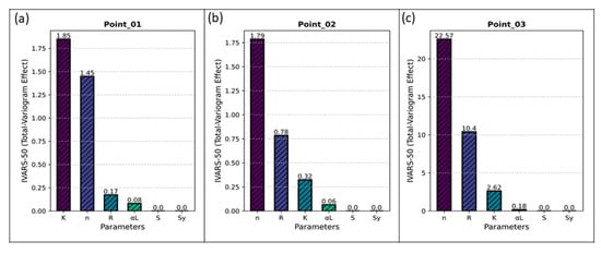
Figure 11.
IVARS-50 sensitivity index results of point 01–point 03 (a–c).
Given the IVARS-50 in Figure 11, hydraulic conductivity (), recharge (), and porosity () were identified as key parameters to assess the impact of uncertainty on the model’s predictions.
The Variogram-based global sensitivity results e.g., directional variogram and sensitivity index IVARS-50 at three different locations of test points show that the substantial influence of hydraulic conductivity, recharge, and porosity on numerical simulation model output (i.e., Cr(VI) concentration), as well as minimal effect of longitudinal dispersivity, specific storage, and specific yield on the Cr(VI) concentration migration.
Hydraulic conductivity plays a direct role in shaping the convective movement of contaminants by affecting pore-fluid velocity. Higher hydraulic conductivity facilitates faster contaminant movement, thereby significantly impacting groundwater transport and resulting in higher contaminant concentrations. Recharge rates significantly influence contaminant concentration by cyclically introducing contaminants into groundwater during water table fluctuations and surface infiltration. Thus, variations in recharge rate directly impact contaminant influx and concentration. Porosity directly impacts the groundwater transport in two key ways: by influencing seepage velocity, which governs convective transport, and by determining the volume of void space available to store groundwater and contaminants. Variations in porosity can lead to changes in the distribution and retention of contaminants, affecting their transport behavior and ultimately impacting contaminant concentration levels in groundwater.
Conversely, longitudinal dispersity, specific storage, and specific yield have a relatively lower sensitivity in influencing contaminant transport. Longitudinal dispersity, although relevant for characterizing the dispersion of contaminants, has minimal influence on contaminant migration. This is attributed to the fact that contaminant dispersion in groundwater, when contrasted with the dominant influence of contaminant convection, is evidently inconsequential. Specific storage and specific yield play a crucial role in regulating groundwater flow dynamics by managing the storage and release of water within the aquifer. However, their impact on contaminant transport, particularly in terms of concentration, may be overshadowed by other parameters such as hydraulic conductivity, recharge, and porosity.
Combining the results in Figure 10 and Figure 11, it is seen that, in proximity to the contaminant source’s location, the magnitude of variations across the perturbation scale and sensitivity index of IVARS-50 is comparatively lower. Conversely, at test points situated farther from the contaminant sources, the magnitude of variations across the perturbation scale and sensitivity index of IVARS-50 exhibits a gradual increase. This phenomenon reflects to the inherent uncertainty associated with the model parameters.
3.3. Evaluation and Comparative Analysis of Surrogate Model Performances
We construct surrogate models for uncertainty estimation of simulation models. To construct robust surrogate models, a total of 300 trials were conducted for hyperparameter optimization using OHPO to systematically explore and search for the optimal combination of hyperparameters [75]. The number of trials are determined by the convergence of searched hyperparameters. As we will see in the results in Section 3.4, this number of trails are enough to build reliable surrogate model within the scope of our study. The MSE, and R2 were chosen as metrics to assess the accuracy of the model during the hyperparameter optimization process. The regularization parameters such as reg_lambda and reg_alpha, are chosen through OHPO, to minimize MSE and maximize the R2 for XGBoost surrogate model. Figure 12 shows the variation of MSE, and R2 during the hyperparameter tuning with the OHPO. The optimal hyperparameters for the model, characterized by the minimum MSE value and a high R2 were identified at the 201st and 265th trial of XGBoost and RF, respectively. The enhancement in performance for XGBoost surrogate model with (OHPO) approach is notably more substantial compared to the improvement observed in the RF surrogate model.
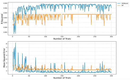
Figure 12.
MSE and R2 across 300 trials of XGBoost and RF during hyperparameter optimization.
Table 4 provides a summary of the optimal hyperparameter values identified through OHPO.

Table 4.
Optimal hyperparameter values captured by Optuna hyperparameter optimization.
The results of accuracy evaluation metrics for the surrogate models have been presented in Table 5. Figure 13 illustrates the fitting curves results, comparing the output of the XGBoost and Random Forest surrogate models with the output of the simulation model. In addition, we conducted a comparison of the accuracy metrics (R2, MSE, RMSE, and MRE) for surrogate models based on individual monitoring wells. The findings are illustrated in Figure 14, indicating a superior performance of the XGBoost surrogate model over the RF surrogate model. Specifically, the R2, MSE, RMSE, and MRE (%) values of surrogate models developed for seventh and eighth Cr(VI) contaminant concentration monitoring wells exceeded those of other monitoring wells. This variation can be attributed to the uncertainty in contaminant concentration output.

Table 5.
Comparison of accuracy of surrogate models.
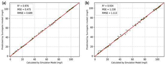
Figure 13.
Fitting curves results of surrogate models: (a) XGBoost; (b) RF.
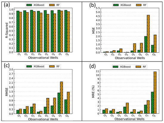
Figure 14.
Accuracy of surrogate models for each monitoring well: (a) R2; (b) MSE; (c) RMSE; (d) MRE (%).
The above results indicate that the XGBoost surrogate model achieved the highest level of accuracy. Hence, due to its superior accuracy, the XGBoost surrogate model has the potential to serve as a replacement for the simulation model in uncertainty analysis.
3.4. Uncertainty Analysis of Groundwater Contaminant Transport
We used the XGBoost as the surrogate model to carry out uncertainty analysis to our simulation model. In GMS 10.6 software, solving the simulation model took about 50 s. The 1000 runs of simulation model for uncertainty analysis took 13.8 h. The surrogate model was established through 140 runs of the simulation model, taking 1.94 h. Employing the surrogate model in the Monte Carlo simulation reduced the calculation time by 85.94%, taking only 4 s.
Utilizing the simulation and surrogate models introduced earlier, we generated 1000 datasets through the application of the Latin Hypercube sampling method. This sampling was conducted within the parameter values’ range identified by global sensitivity analysis in the model. The outcomes of the sampling were input into the trained surrogate model to conduct a Monte Carlo simulation. Subsequently, the statistical analysis of the Cr(VI) concentration in the output from individual monitoring wells was performed using SPSS software (version 22). Frequency histograms of Cr(VI) concentration in each monitoring well are shown in Figure 15.
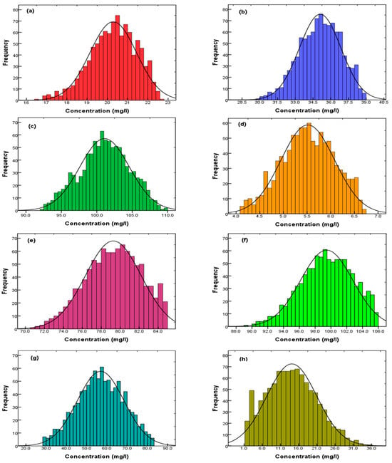
Figure 15.
Frequency histograms of Cr(VI) concentration in each monitoring well O1–O8 (a–h).
Figure 15a,b,d demonstrate that the uncertainty resulting from variability in key parameters had a lesser impact on wells O1, O2, and O4, which were in close proximity to the contaminant source. In contrast, Figure 15g,h indicate a significant impact on wells O8, and O7, positioned at a considerable distance from the contaminant source.
In uncertainty analysis, standard deviation plays a crucial role in quantifying the uncertainty or variability associated with a set of measurements, observations, or model predictions. Results of standard deviation are presented in Table 6. A higher standard deviation implies greater dispersion in the outputs, signifying increased uncertainty. Owing to the stochastic nature of key parameters, the Cr(VI) concentration in each well exhibited significant variations.

Table 6.
Statistical summary of concentration output values for contaminant in monitoring wells.
Among the monitoring wells, O4, O1, and O2 exhibited the least discreteness in their outputs, while O7 and O8 displayed the highest discreteness. This suggests that the later wells were more significantly influenced by the variability of the key parameters.
In the SPSS software, we also calculated the confidence intervals for Cr(VI) ion concentrations in each well at confidence levels of 60% and 90%. In the context of uncertainty analysis, confidence intervals are useful for conveying the precision or uncertainty associated with estimates, predictions, or model outcomes. The width of the confidence interval reflects the level of uncertainty: a wider interval suggests greater uncertainty, while a narrower interval implies more precision in the estimate.
As shown in Table 7, well O7 exhibited the widest confidence interval among all considered wells for the identical confidence level. At a confidence level of 90%, the confidence interval for well O7 ranged from 56.31 to 57.51 mg/L, highlighting its heightened susceptibility to uncertainty in the three key parameters. Conversely, the confidence interval for O4 was the smallest, indicating that it is less susceptible to uncertainty in these key parameters. Thus, the confidence interval results indicate that as the confidence level increases, the interval range also increases; conversely, as the confidence level decreases, the interval range diminishes, resulting in a more concentrated distribution around the mean.

Table 7.
Interval estimation for each contaminant monitoring well.
In summary, the uncertainty analysis shows how the variability of key parameters affect the simulation results. This helps us to figure out the best ways to improve simulation accuracy for ensuring the reliability of our model’s predictions.
This study’s findings suggest the critical need to strategically place repair measures, like implementing a Permeable Reactive Barrier (PRB) and Pumping Wells, to reduce the Cr(VI) contamination downstream. Wells closer to the contamination source show less variability, indicating that they are less influenced by key parameters. Hence, prioritizing remediation efforts near the source, specifically at monitoring wells O1, O2, and O4, is crucial. Installing PRBs at these locations holds significant promise in intercepting and treating the contaminant plume. Continuous monitoring of these wells is vital to assess the effectiveness of the remediation interventions.
Given the wider confidence intervals observed in monitoring wells positioned farther from the contamination source, such as O7, addressing simulation uncertainties becomes crucial, particularly focusing on PRB placement. Uncertainty in PRB placement could greatly impact its effectiveness in intercepting and treating the contaminant plume. Therefore, reducing simulation uncertainties, particularly regarding PRB deployment, is essential to ensure the precision and reliability of remediation strategies targeting Cr(VI) contamination reduction. This, in turn, effectively protects groundwater quality and public health.
4. Conclusions
In this study, we propose a Variogram-based Global Sensitivity Analysis (VARS) to identify the most influential parameters affecting the numeric simulation model output, serving as key parameters. Based on these key parameters, an XGBoost surrogate model was established for approximating the inherent association between groundwater parameters and contaminants distribution. This approach aimed to reduce the computational burden of Monte Carlo simulation for uncertainty analysis while maintaining the accuracy of the model predictions.
The following conclusions can be made:
- (1)
- Through global sensitivity analysis, hydraulic conductivity (), recharge (), and porosity () were identified as the key parameters to conduct the comprehensive evaluation of uncertainty’s impact on numeric simulation model results. Sensitivity analysis serves a dual purpose by diminishing the input dimensions of the surrogate model, thereby enhancing its precision, and providing guidance for the investigation of contaminated site.
- (2)
- During the uncertainty analysis, an XGBoost-based surrogate model not only effectively captured the non-linear correlations between input and output of the numeric simulation model, but also markedly mitigated computational workload and calculation time. Using an XGBoost-based surrogate model, instead of directly calling the numeric simulation model leads to an 85.94% reduction in computation time, making the Monte Carlo simulation with this surrogate model viable and efficient.
- (3)
- Utilizing the Monte Carlo simulation to consider the impact of random variations of key parameters on the numeric simulation model, results showed how later wells were influenced by the variability in the key parameters, which provided insights for improving the accuracy of groundwater simulation.
- (4)
- The Numeric Simulation model illustrated that the movement of the Cr(VI) contaminant plume is toward downstream. In order to effectively reduce the risk of chromium pollution in the downstream area, some pollution remediation measures such as PRB and pumping wells are suggested be set in the downstream location of the site.
In future studies, we’ll develop Auto Machine Learning (ML) method to automate model selection and hyperparameter optimization in machine learning engineering, reducing human intervention and saving time in the process of simulation. However, the current simulation lacks validation against independently measured values of concentrations, emphasizing the need for a rigorous validation step. Such validation is indispensable for ensuring the reliability and accuracy of our model’s predictions by benchmarking them against real-world data.
Author Contributions
Conceptualization, Y.Z., H.D. and M.S.Y.; methodology, Y.Z, M.S.Y. and F.Y.; software, F.Y. and M.S.Y.; validation, Y.Z., H.D. and F.Y.; data curation, M.S.Y., F.Y. and Y.H.; writing—original draft preparation, Y.Z. and M.S.Y.; writing—review and editing, H.D. and Y.H.; funding acquisition, Y.Z. and H.D. All authors have read and agreed to the published version of the manuscript.
Funding
This study was supported by grants from the National Key Research and Development Program of China (Grant No. 2019YFC1805905), the National Natural Science Foundation of China (Grant Nos. 42372346, 41872249 and 42272344).
Data Availability Statement
The datasets presented in this article are not readily available because the data are part of an ongoing study. Requests to access the datasets should be directed to corresponding author.
Conflicts of Interest
The authors declare no conflicts of interest.
References
- Banaei, S.M.A.; Javid, A.H.; Hassani, A.H. Numerical Simulation of Groundwater Contaminant Transport in Porous Media. Int. J. Environ. Sci. Technol. 2021, 18, 151–162. [Google Scholar] [CrossRef]
- Rahman, S.H.; Khanam, D.; Adyel, T.M.; Islam, M.S.; Ahsan, M.A.; Akbor, M.A. Assessment of Heavy Metal Contamination of Agricultural Soil around Dhaka Export Processing Zone (DEPZ), Bangladesh: Implication of Seasonal Variation and Indices. Appl. Sci. 2012, 2, 584. [Google Scholar] [CrossRef]
- Chen, R.; Teng, Y.; Chen, H.; Yue, W.; Su, X.; Liu, Y.; Zhang, Q. A Coupled Optimization of Groundwater Remediation Alternatives Screening under Health Risk Assessment: An Application to a Petroleum-Contaminated Site in a Typical Cold Industrial Region in Northeastern China. J. Hazard. Mater. 2021, 407, 124796. [Google Scholar] [CrossRef]
- He, Q.; He, Y.; Hu, H.; Lou, W.; Zhang, Z.; Zhang, K.; Chen, Y.; Ye, W.; Sun, J. Laboratory Investigation on the Retention Performance of a Soil–Bentonite Mixture Used as an Engineered Barrier: Insight into the Effects of Ionic Strength and Associated Heavy Metal Ions. Environ. Sci. Pollut. Res. 2023, 30, 50162–50173. [Google Scholar] [CrossRef]
- Zhu, F.; Liu, T.; Zhang, Z.; Liang, W. Remediation of Hexavalent Chromium in Column by Green Synthesized Nanoscale Zero-Valent Iron/Nickel: Factors, Migration Model and Numerical Simulation. Ecotoxicol. Environ. Saf. 2021, 207, 111572. [Google Scholar] [CrossRef]
- Xu, X.; Huang, H.; Zhang, Y.; Xu, Z.; Cao, X. Biochar as Both Electron Donor and Electron Shuttle for the Reduction Transformation of Cr(VI) during Its Sorption. Environ. Pollut. 2019, 244, 423–430. [Google Scholar] [CrossRef]
- Xu, Z.; Xu, X.; Tao, X.; Yao, C.; Tsang, D.C.W.; Cao, X. Interaction with Low Molecular Weight Organic Acids Affects the Electron Shuttling of Biochar for Cr(VI) Reduction. J. Hazard. Mater. 2019, 378, 120705. [Google Scholar] [CrossRef] [PubMed]
- DesMarias, T.L.; Costa, M. Mechanisms of Chromium-Induced Toxicity. Curr. Opin. Toxicol. 2019, 14, 1–7. [Google Scholar] [CrossRef] [PubMed]
- Zhang, N.; Fang, Z.; Zhang, R. Comparison of Several Amendments for In-Site Remediating Chromium-Contaminated Farmland Soil. Water Air Soil Pollut. 2017, 228, 400. [Google Scholar] [CrossRef]
- He, Q.; He, Y.; Zhang, Z.; Ou, G.; Zhu, K.; Lou, W.; Zhang, K.; Chen, Y.; Ye, W. Spatiotemporal Distribution and Pollution Control of Pollutants in a Cr(VI)-Contaminated Site Located in Southern China. Chemosphere 2023, 340, 139897. [Google Scholar] [CrossRef]
- He, Y.; Hu, G.; Wu, D.; Zhu, K.; Zhang, K. Contaminant Migration and the Retention Behavior of a Laterite–Bentonite Mixture Engineered Barrier in a Landfill. J. Environ. Manag. 2022, 304, 114338. [Google Scholar] [CrossRef]
- Deng, H.; Zhou, S.; He, Y.; Lan, Z.; Zou, Y.; Mao, X. Efficient Calibration of Groundwater Contaminant Transport Models Using Bayesian Optimization. Toxics 2023, 11, 438. [Google Scholar] [CrossRef]
- Liu, L.; Liang, S.; Liu, H.; Tan, W.; Zhu, G. Migration of and Butanone in Soil and Groundwater System After the Tianjin Port 8·12 Explosion. Trans. Tianjin Univ. 2018, 24, 522–531. [Google Scholar] [CrossRef]
- He, Y.; Hu, G.; Zhang, Z.; Lou, W.; Zou, Y.; Li, X.; Zhang, K. Experimental Study and Numerical Simulation on the Migration and Transformation Mechanism of Hexavalent Chromium in Contaminated Site. Rock Soil Mech. 2022, 43, 528–538. [Google Scholar] [CrossRef]
- Wu, X.; Ye, T.; Xie, C.; Li, K.; Liu, C.; Yang, Z.; Han, R.; Wu, H.; Wang, Z. Experimental and Modeling Study on Cr(VI) Migration from Slag into Soil and Groundwater. Processes 2022, 10, 2235. [Google Scholar] [CrossRef]
- Guo, S.; Xu, Y.; Yang, J. Simulating the Migration and Species Distribution of Cr and Inorganic Ions from Tanneries in the Vadose Zone. J. Environ. Manag. 2021, 288, 112441. [Google Scholar] [CrossRef] [PubMed]
- Liu, L.; Xiao, L.; Li, X. Simulation of Migration of Hexavalent Chromium in Groundwater. Xitong Fangzhen Xuebao/J. Syst. Simul. 2018, 30, 560–568. [Google Scholar] [CrossRef]
- Xue, L.; Zhang, D.; Guadagnini, A.; Neuman, S.P. Multimodel B Ayesian Analysis of Groundwater Data Worth. Water Resour. Res. 2014, 50, 8481–8496. [Google Scholar] [CrossRef]
- Chitsazan, N.; Nadiri, A.A.; Tsai, F.T.-C. Prediction and Structural Uncertainty Analyses of Artificial Neural Networks Using Hierarchical Bayesian Model Averaging. J. Hydrol. 2015, 528, 52–62. [Google Scholar] [CrossRef]
- Moazamnia, M.; Hassanzadeh, Y.; Nadiri, A.A.; Khatibi, R.; Sadeghfam, S. Formulating a Strategy to Combine Artificial Intelligence Models Using Bayesian Model Averaging to Study a Distressed Aquifer with Sparse Data Availability. J. Hydrol. 2019, 571, 765–781. [Google Scholar] [CrossRef]
- Troldborg, M.; Nowak, W.; Tuxen, N.; Bjerg, P.L.; Helmig, R.; Binning, P.J. Uncertainty Evaluation of Mass Discharge Estimates from a Contaminated Site Using a Fully Bayesian Framework. Water Resour. Res. 2010, 46, 2010WR009227. [Google Scholar] [CrossRef]
- Delottier, H.; Pryet, A.; Dupuy, A. Why Should Practitioners Be Concerned about Predictive Uncertainty of Groundwater Management Models? Water Resour. Manag. 2017, 31, 61–73. [Google Scholar] [CrossRef]
- Nemati, M.; Tabari, M.M.R.; Hosseini, S.A.; Javadi, S. A Novel Approach Using Hybrid Fuzzy Vertex Method-MATLAB Framework Based on GMS Model for Quantifying Predictive Uncertainty Associated with Groundwater Flow and Transport Models. Water Resour. Manag. 2021, 35, 4189–4215. [Google Scholar] [CrossRef]
- Troldborg, L.; Ondracek, M.; Koch, J.; Kidmose, J.; Refsgaard, J.C. Quantifying Stratigraphic Uncertainty in Groundwater Modelling for Infrastructure Design. Hydrogeol. J. 2021, 29, 1075–1089. [Google Scholar] [CrossRef]
- Bordbar, M.; Neshat, A.; Javadi, S. A New Hybrid Framework for Optimization and Modification of Groundwater Vulnerability in Coastal Aquifer. Environ. Sci. Pollut. Res. 2019, 26, 21808–21827. [Google Scholar] [CrossRef] [PubMed]
- Yan, X.; Lu, W.; An, Y.; Chang, Z. Uncertainty Analysis of Parameters in Non-Point Source Pollution Simulation: Case Study of the Application of the Soil and Water Assessment Tool Model to Yitong River Watershed in Northeast China. Water Environ. J. 2019, 33, 390–400. [Google Scholar] [CrossRef]
- Xing, Y.; Shao, D.; Yang, Y.; Ma, X.; Zhang, S. Influence and Interactions of Input Factors in Urban Flood Inundation Modeling: An Examination with Variance-Based Global Sensitivity Analysis. J. Hydrol. 2021, 600, 126524. [Google Scholar] [CrossRef]
- van Griensven, A.; Meixner, T.; Grunwald, S.; Bishop, T.; Diluzio, M.; Srinivasan, R. A Global Sensitivity Analysis Tool for the Parameters of Multi-Variable Catchment Models. J. Hydrol. 2006, 324, 10–23. [Google Scholar] [CrossRef]
- Tansar, H.; Duan, H.-F.; Mark, O. Global Sensitivity Analysis of Bioretention Cell Design for Stormwater System: A Comparison of VARS Framework and Sobol Method. J. Hydrol. 2023, 617, 128895. [Google Scholar] [CrossRef]
- Nolan, B.T.; Healy, R.W.; Taber, P.E.; Perkins, K.; Hitt, K.J.; Wolock, D.M. Factors Influencing Ground-Water Recharge in the Eastern United States. J. Hydrol. 2007, 332, 187–205. [Google Scholar] [CrossRef]
- Hornberger, G.M.; Spear, R.C. Approach to the Preliminary Analysis of Environmental Systems. J. Environ. Manag. 1981, 12, 7–18. [Google Scholar]
- Morris, M.D. Factorial Sampling Plans for Preliminary Computational Experiments. Technometrics 1991, 33, 161–174. [Google Scholar] [CrossRef]
- Sobolprime, I.M. Sensitivity Analysis for Non-Linear Mathematical Models. Math. Model. Comput. Exp. 1993, 1, 407–414. [Google Scholar]
- Razavi, S.; Gupta, H.V. A New Framework for Comprehensive, Robust, and Efficient Global Sensitivity Analysis: 1. Theory. Water Resour. Res. 2016, 52, 423–439. [Google Scholar] [CrossRef]
- Razavi, S.; Gupta, H.V. A New Framework for Comprehensive, Robust, and Efficient Global Sensitivity Analysis: 2. Application. Water Resour. Res. 2016, 52, 440–455. [Google Scholar] [CrossRef]
- Loucks, D.P.; van Beek, E. System Sensitivity and Uncertainty Analysis. In Water Resource Systems Planning and Management; Springer: Cham, Switzerland, 2017; pp. 331–374. ISBN 978-3-319-44234-1. [Google Scholar]
- Jiang, X.; Na, J.; Lu, W.; Zhang, Y. Coupled Monte Carlo Simulation and Copula Theory for Uncertainty Analysis of Multiphase Flow Simulation Models. Environ. Sci. Pollut. Res. 2017, 24, 24284–24296. [Google Scholar] [CrossRef] [PubMed]
- Zhang, Z.; Wang, X.; Li, M. Uncertainty analysis of WASP based on global sensitivity analysis method. China Environ. Sci. 2014, 34, 1336–1346. [Google Scholar]
- Luo, J.; Liu, Y.; Li, X.; Xin, X.; Lu, W. Inversion of Groundwater Contamination Source Based on a Two-Stage Adaptive Surrogate Model-Assisted Trust Region Genetic Algorithm Framework. Appl. Math. Model. 2022, 112, 262–281. [Google Scholar] [CrossRef]
- Li, S.; Farrar, C.; Yang, Y. Efficient Regional Seismic Risk Assessment via Deep Generative Learning of Surrogate Models. Earthq. Eng. Struct. Dyn. 2023, 52, 3435–3454. [Google Scholar] [CrossRef]
- Rajabi, M.M. Review and Comparison of Two Meta-Model-Based Uncertainty Propagation Analysis Methods in Groundwater Applications: Polynomial Chaos Expansion and Gaussian Process Emulation. Stoch Environ. Res. Risk Assess. 2019, 33, 607–631. [Google Scholar] [CrossRef]
- Stone, N. Gaussian Process Emulators for Uncertainty Analysis in Groundwater Flow. Ph.D. Thesis, University of Nottingham, Nottingham, UK, 2011. [Google Scholar]
- Miao, T.; Lu, W.; Lin, J.; Guo, J.; Liu, T. Modeling and Uncertainty Analysis of Seawater Intrusion in Coastal Aquifers Using a Surrogate Model: A Case Study in Longkou, China. Arab. J. Geosci. 2018, 12, 1. [Google Scholar] [CrossRef]
- Miao, T.; Lu, W.; Luo, J.; Guo, J. Application of Set Pair Analysis and Uncertainty Analysis in Groundwater Pollution Assessment and Prediction: A Case Study of a Typical Molybdenum Mining Area in Central Jilin Province, China. Environ. Earth Sci. 2019, 78, 323. [Google Scholar] [CrossRef]
- Miao, T.; Lu, W.; Guo, J.; Lin, J.; Fan, Y. Modeling and Uncertainty Analysis of Seawater Intrusion Based on Surrogate Models. Environ. Sci. Pollut. Res. 2019, 26, 26015–26025. [Google Scholar] [CrossRef] [PubMed]
- Fan, Y.; Wu, Q.; Cui, H.; Lu, W.; Ren, W. Stochastic Simulation of Seawater Intrusion in the Longkou Area of China Based on the Monte Carlo Method. Environ. Sci. Pollut. Res. 2023, 30, 22063–22077. [Google Scholar] [CrossRef] [PubMed]
- Thiros, N.E.; Gardner, W.P.; Maneta, M.P.; Brinkerhoff, D.J. Quantifying Subsurface Parameter and Transport Uncertainty Using Surrogate Modelling and Environmental Tracers. Hydrol. Process. 2022, 36, e14743. [Google Scholar] [CrossRef]
- Han, Z.; Lu, W.; Lin, J. Uncertainty Analysis for Precipitation and Sea-Level Rise of a Variable-Density Groundwater Simulation Model Based on Surrogate Models. Environ. Sci. Pollut. Res. 2020, 27, 28077–28090. [Google Scholar] [CrossRef] [PubMed]
- Fan, Y.; Lu, W.; Miao, T.; Li, J.; Lin, J. Optimum Design of a Seawater Intrusion Monitoring Scheme Based on the Image Quality Assessment Method. Water Resour. Manag. 2020, 34, 2485–2502. [Google Scholar] [CrossRef]
- Špetlík, M.; Březina, J. Groundwater Contaminant Transport Solved by Monte Carlo Methods Accelerated by Deep Learning Meta-Model. Appl. Sci. 2022, 12, 7382. [Google Scholar] [CrossRef]
- Miao, T.; Huang, H.; Guo, J.; Li, G.; Zhang, Y.; Chen, N. Uncertainty Analysis of Numerical Simulation of Seawater Intrusion Using Deep Learning-Based Surrogate Model. Water 2022, 14, 2933. [Google Scholar] [CrossRef]
- Yu, X.; Cui, T.; Sreekanth, J.; Mangeon, S.; Doble, R.; Xin, P.; Rassam, D.; Gilfedder, M. Deep Learning Emulators for Groundwater Contaminant Transport Modelling. J. Hydrol. 2020, 590, 125351. [Google Scholar] [CrossRef]
- Wang, R.-Z.; Gu, H.-H.; Liu, Y.; Miura, H.; Zhang, X.-C.; Tu, S.-T. Surrogate-Modeling-Assisted Creep-Fatigue Reliability Assessment in a Low-Pressure Turbine Disc Considering Multi-Source Uncertainty. Reliab. Eng. Syst. Saf. 2023, 240, 109550. [Google Scholar] [CrossRef]
- Zhang, L.; Lin, P. Multi-Objective Optimization for Limiting Tunnel-Induced Damages Considering Uncertainties. Reliab. Eng. Syst. Saf. 2021, 216, 107945. [Google Scholar] [CrossRef]
- Aquaveo, LLC. Groundwater Modeling System (GMS, v.10.6). Available online: https://www.aquaveo.com/downloads-gms (accessed on 10 November 2023).
- He, H.; Shan, H.; Mo, D.; Liu, Y.; Peng, S.; Cheng, Y.; Chen, M.; Yan, Z. Simulation Study on the Environmental Impact of Rare Earth Ore Development on Groundwater in Hilly Areas: A Case Study in Nuodong, China. Water 2023, 15, 263. [Google Scholar] [CrossRef]
- Rabemaharitra, T.P.; Zou, Y.; Yi, Z.; He, Y.; Khan, U. Optimized Pilot Point Emplacement Based Groundwater Flow Calibration Method for Heterogeneous Small-Scale Area. Appl. Sci. 2022, 12, 4648. [Google Scholar] [CrossRef]
- Konikow, L.F. The Secret to Successful Solute-Transport Modeling. Ground Water 2011, 49, 144–159. [Google Scholar] [CrossRef] [PubMed]
- Kresic, N. Hydrogeology and Groundwater Modeling, 2nd ed.; CRC Press: Boca Raton, FL, USA, 2006; ISBN 978-0-429-12210-1. [Google Scholar]
- Zheng, C.; Bennett, G. Applied Contaminant Transport Modeling; Wiley-Interscience: New York, NY, USA, 2002; Volume 34, ISBN 978-0-471-38477-9. [Google Scholar]
- Liu, L.; Chen, J.; Niu, H.; Li, L.; Yin, L.; Wei, Y. Numerical simulation of three-dimensional soil-groundwater coupled chromium contamination based on FEFLOW. Hydrogeol. Eng. Geol. 2022, 49, 164–174. [Google Scholar] [CrossRef]
- Razavi, S.; Gupta, H.V. A Multi-Method Generalized Global Sensitivity Matrix Approach to Accounting for the Dynamical Nature of Earth and Environmental Systems Models. Environ. Model. Softw. 2019, 114, 1–11. [Google Scholar] [CrossRef]
- Haghnegahdar, A.; Razavi, S. Insights into Sensitivity Analysis of Earth and Environmental Systems Models: On the Impact of Parameter Perturbation Scale. Environ. Model. Softw. 2017, 95, 115–131. [Google Scholar] [CrossRef]
- Sheikholeslami, R.; Razavi, S. Progressive Latin Hypercube Sampling: An Efficient Approach for Robust Sampling-Based Analysis of Environmental Models. Environ. Model. Softw. 2017, 93, 109–126. [Google Scholar] [CrossRef]
- Chen, T.; Guestrin, C. XGBoost: A Scalable Tree Boosting System. In Proceedings of the 22nd ACM SIGKDD International Conference on Knowledge Discovery and Data Mining, San Francisco, CA, USA, 13–17 August 2016; pp. 785–794. [Google Scholar]
- Yan, Y.; Li, X.; Sun, W.; Fang, X.; He, F.; Tu, J. Semi-Surrogate Modelling of Droplets Evaporation Process via XGBoost Integrated CFD Simulations. Sci. Total Environ. 2023, 895, 164968. [Google Scholar] [CrossRef]
- Chen, Y.; Li, F.; Zhou, S.; Zhang, X.; Zhang, S.; Zhang, Q.; Su, Y. Bayesian Optimization Based Random Forest and Extreme Gradient Boosting for the Pavement Density Prediction in GPR Detection. Constr. Build. Mater. 2023, 387, 131564. [Google Scholar] [CrossRef]
- Breiman, L. Random Forests. Mach. Learn. 2001, 45, 5–32. [Google Scholar] [CrossRef]
- Tian, L.; Hu, L.; Wang, D.; Cao, X. Site-Scale Groundwater Pollution Risk Assessment Using Surrogate Models and Statistical Analysis. J. Contam. Hydrol. 2024, 261, 104288. [Google Scholar] [CrossRef] [PubMed]
- Iman, R.L. Latin Hypercube Sampling. In Encyclopedia of Quantitative Risk Analysis and Assessment; Melnick, E.L., Everitt, B.S., Eds.; Wiley: Hoboken, NJ, USA, 2008; ISBN 978-0-470-03549-8. [Google Scholar]
- Akiba, T.; Sano, S.; Yanase, T.; Ohta, T.; Koyama, M. Optuna: A Next-Generation Hyperparameter Optimization Framework. In Proceedings of the 25th ACM SIGKDD International Conference on Knowledge Discovery & Data Mining, San Francisco, CA, USA, 4–8 August 2019; Association for Computing Machinery: New York, NY, USA, 2019; pp. 2623–2631. [Google Scholar]
- Luo, J.; Ma, X.; Ji, Y.; Li, X.; Song, Z.; Lu, W. Review of Machine Learning-Based Surrogate Models of Groundwater Contaminant Modeling. Environ. Res. 2023, 238, 117268. [Google Scholar] [CrossRef]
- Xie, W.; Nelson, B.L.; Barton, R.R. Statistical Uncertainty Analysis for Stochastic Simulation. arXiv 2020, arXiv:2011.04207. [Google Scholar] [CrossRef]
- Zhang, J. Modern Monte Carlo Methods for Efficient Uncertainty Quantification and Propagation: A Survey. WIREs Comput. Stats 2021, 13, e1539. [Google Scholar] [CrossRef]
- Pan, Z.; Lu, W.; Wang, H.; Bai, Y. Groundwater Contaminant Source Identification Based on an Ensemble Learning Search Framework Associated with an Auto Xgboost Surrogate. Environ. Model. Softw. 2023, 159, 105588. [Google Scholar] [CrossRef]
Disclaimer/Publisher’s Note: The statements, opinions and data contained in all publications are solely those of the individual author(s) and contributor(s) and not of MDPI and/or the editor(s). MDPI and/or the editor(s) disclaim responsibility for any injury to people or property resulting from any ideas, methods, instructions or products referred to in the content. |
© 2024 by the authors. Licensee MDPI, Basel, Switzerland. This article is an open access article distributed under the terms and conditions of the Creative Commons Attribution (CC BY) license (https://creativecommons.org/licenses/by/4.0/).