
An Investigation of Contaminant Transport and Retention from Storage Zone in Meandering Channels

1
Department of Civil and Environmental Engineering, Yonsei University, 50, Yonsei-ro, Seodaemun-gu, Seoul 03722, Republic of Korea
2
Department of Civil Engineering, Seoul National University of Science and Technology (SeoulTech), 232, Gongneung-ro, Nowon-gu, Seoul 01811, Republic of Korea
3
Department of Civil and Environmental Engineering, Gachon University, 1342, SeongnamDaero, Sujeong-gu, Seongnam-si 13120, Republic of Korea
*
Author to whom correspondence should be addressed.
Water 2024, 16(8), 1170; https://doi.org/10.3390/w16081170
Submission received: 21 March 2024
/
Revised: 16 April 2024
/
Accepted: 18 April 2024
/
Published: 20 April 2024
(This article belongs to the Special Issue Contaminant Transport Modeling in Aquatic Environments)
Abstract
:Contaminant trapping by recirculation zones occurring at the apex of natural meandering channels induces a long tail in the contaminant cloud, thereby complicating the prediction of mixing behaviors. Thus, the understanding of the interaction between solute trapping and recirculating flow is important for responding to and mitigating water pollution accidents. In this research, the EFDC model was employed to reproduce three-dimensional flow structures of recirculating flow at the channel apex and investigate the influence on contaminant mixing. To investigate the contaminant transport characteristics from the storage zone in meandering channels, simulations were conducted using various discharge values to assess the impact of storage zone development on the concentration–time curves. The analysis of the relationship between the storage zone size and mixing behaviors indicates that an increase in discharge could result in a shorter tail and larger longitudinal dispersion even with the larger storage zone size. On the other hand, the enlarged recirculation zone size contributes to reducing transverse dispersion, evidenced by flatter dosage curves under lower flow rate conditions. These findings suggest that the increase in longitudinal dispersion with a larger flow rate is primarily caused by the reduction in transverse dispersion resulting from the formation of the recirculation zone.
1. Introduction
Rivers are dynamic systems of nature that have meandering curves and sinuous channel patterns. These meandering shapes of rivers significantly influence the topography and flow dynamics of water flow. Meandering rivers are characterized by continuous lateral shifts in their channels, giving rise to patterns that influence the velocity and behavior of water flow within them [1]. This induces complex flow characteristics including secondary flows and recirculation zones, which have significant effects on the transport of contaminants within rivers. In meandering rivers, the flow velocity creates recirculation, which forms complex patterns of water movement and secondary flows [2]. One notable feature associated with meandering river channels is the development of helical secondary flows [3,4,5]. These helical flows, which resemble corkscrew patterns, contribute to mixing within the river. Understanding the role of these flow characteristics is essential for comprehending the complex transport processes occurring in meandering rivers [6].
Furthermore, riverine dynamics are further complicated by the existence of flow recirculation zones in meandering rivers. Tracers and other materials carried by the flowing water are captured in these recirculation zones [7]. As a result, the movement of these tracers in the river becomes complex, and there is a chance that tracer concentration will be abnormally high at both the early and late stages of breakthrough curves due to captured tracers. Investigating these breakthrough curves can provide insights into the temporal evolution of tracer concentrations [8,9], which may offer valuable information about the transport mechanisms influenced by meander-driven flows.
Figure 1 depicts the mixing processes in a meandering river and their effects on solute transport, as indicated by the distribution of concentrations over time at different sections of the river. Section A is located at the inner bend of the meander where the water flow is faster due to the narrower path, which leads to the erosion of the riverbank and the formation of a steep cut bank. Between Section A and Section B is the outer bend where the water flow is slower and is characterized by deep water and recirculating flow. The contaminant transport in these meander-type areas produces concentration–time curves displayed at the right area of the figure, where a Fickian distribution is observed in Section A, which is typically symmetric and bell-shaped [10]. This suggests that the solute is well mixed in this section of the river, and there is an equilibrium between the shear and diffusion processes. The solute concentration increases quickly to a peak and then decreases at the same rate. Section B’s graph is a non-Fickian distribution with a long tail. This suggests complex mixing, possibly due to the slower flow and recirculation that occurred between Section A and Section B. The peak concentration is lower, and the return to the baseline concentration is slower, as indicated by the long tail. This long tail exhibits that the solute is retained longer in the outside bend of the river, and therefore the storage effect is caused by the slower flow and recirculation.
To analyze the introduced characteristic of pollutant transport in meandering rivers, contaminant transport models can be used [11]. These models are utilized as decision-making tools for controlling water quality, assessing current conditions, and responding to chemical accidents. To operate and use contaminant transport models, knowledge about the parameters and processes related to modeling such as contaminant dispersion is required. There are several methods for modeling contaminant transport, including advection and dispersion equation modeling [12]. Advection and dispersion equation modeling is a method that reproduces the contaminant transport through dispersion, and it requires parameters such as the dispersion coefficient.
There are multiple methods for estimating dispersion coefficients, which usually use the observed concentration data curves from conducted tracer field experiments for analysis [13]. These methods based on observed data use theoretical and empirical approaches. The theoretical methods are based on the dispersion theory [14], which is the main reason for concentration spread for transverse mixing throughout the channel. The empirical methods usually utilize a regression technique based on the basic parameters of natural rivers, such as hydraulic radius, depth, width, and geometric parameters using dimensional analysis [15]. Flow structures created by geometrical and hydrologic properties would influence the mixing process due to the creation of the recirculation zone and secondary flows.
The aim of this study is to investigate how discharge changes could affect the size of the storage zone in rivers caused by channel meanders and how they affect the movement of contaminants. By examining the connection between complex flow patterns involving storage zones with meandering rivers, we seek to find the factors contributing to mixing aspects of tracer and concentration changes. Through the exploration of storage zone sizes by meander-driven flows, we aim to develop an understanding of flow dynamics and their effects on contaminant transport in natural rivers. Therefore, we conducted this research as follows: Tracer test results presented by Kim et al. [16] in a natural river were used for validating the contaminant transport model. Next, the quasi-three-dimensional flow analysis model was used to conduct continuous simulations with various discharges to find how different flow cases affect the storage zones in meandering rivers. Then, a detailed analysis of the characteristics of the concentration curve based on changes to the flow conditions, and changes in the storage size (length and width) according to the flow rate change, and a comparison of dispersion coefficient calculation results were conducted.
2. Background Theory and Methodology
2.1. Longitudinal Mixing Process
To analyze longitudinal mixing, many attempts using derivation with equations based on observed tracer tests or models have been made [17,18]. When contaminants are discharged into the river, they go through advective and dispersive transport processes as the water flows downstream. Most rivers have a large aspect ratio with a larger lateral width than the water depth, causing the vertical and lateral process of cross-sectional mixing to be completed in a short period [19]. Therefore, the one-dimensional (1D) model derived by Taylor [20] is generally used in the river mixing analysis. The governing equation of the 1D model can be written as follows:
where C is the cross-sectional average concentration; U is the cross-sectional average velocity; K is the longitudinal dispersion coefficient; and t is the time. The longitudinal dispersion coefficient K is the most important parameter in applying Equation (1) describing the spreading of contaminants downstream within a flow in a river, with higher values indicating more mixing and spreading. To calculate longitudinal dispersion coefficients, many attempts have been made based on observed data from tracer tests [13,15,21,22].
In this study, the moment method, which is commonly used for estimating the longitudinal dispersion coefficient, was applied. The moment method is based on the assumption that the rate of change in variance is proportional to the longitudinal dispersion coefficient. The equation of the moment method is given as follows [23,24]:
where Li is the longitudinal distance from the injection point to section i; is the centroid of the concentration–time curve; is the variance of the concentration distribution of section i which can be calculated from the moment relationship of concentration–time curve as follows:
where Mi is the i-th moment of the concentration–time curve; μ is the mean. From Equations (4) and (5), variance can be calculated by using Equation (6) [25].
However, most natural rivers have complex geometry with irregular channel boundaries, and storage zones are generated from various factors [26]. These storage zones lead to the recirculation and stagnation of water, which induce the entrapment of contaminants. This process explains the skewness of the observed concentration distribution with long tailing at the falling limb of the concentration–time curve. Reflecting these effects in the mixing process, the storage zone model explains the relationship between the impact of solute trapping in the recirculation zone and longitudinal dispersion, and the equation is given as follows:
where Cs is the concentration in the recirculation zone; Ks is the longitudinal dispersion coefficient excluding storage effects; is the area ratio of storage and flow zones; and is the residence time in the storage zone.
2.2. Numerical Model Descriptions
To evaluate the retention of contaminant in meandering channels by modeling a meandering river with different discharge conditions and estimating longitudinal coefficients using the introduced moment method, the Environmental Fluid Dynamics Code (EFDC) developed by the Virginia Institute of Technology was used in this study [27]. The EFDC is the quasi-three-dimensional hydrodynamic model assuming the hydrostatic condition for the momentum equation in the vertical direction. The model uses the Reynolds-averaged Navier–Stokes equation as the governing equation of flow analysis. The turbulence closure of the horizontal momentum equation was modeled using the Smagorinsky model, whereas the vertical momentum equation was modeled using the Mellor–Yamada turbulence model. Explicit and implicit time-discretizing methods were used, and the model used the finite-difference method to discretize the governing equation. The mass transport model uses the advection–diffusion equation as a governing equation given below.
where is the time-averaged concentration; is water depth; , , and are the time-averaged velocity components; and are the horizontal and vertical turbulent diffusion coefficients, respectively. The mass transport model is fully coupled with the flow analysis model. Under the Reynolds analogy assumption, the turbulent diffusion coefficient is thus equal to the eddy viscosity terms, as determined by the turbulence closure models. This model has been applied to various rivers, lakes, and aquatic environments [28]. With its capability of flow modeling and contaminant transport modeling, a modeling framework based on the EFDC was established to simulate the spatial–temporal variability and transportation mechanism of contaminants such as PCBs [29]. The model also displayed its capabilities in modeling water quality in urban lakes [30]. Additionally, the results of the models could be used for the risk assessment of water quality such as estimating the risk of hazardous materials loading into aquatic environments [31]. Overall, this model is suitable for river and lake modeling, as the USEPA listed the EFDC model as a tool for water quality management [32].
3. Target Area and Methods
3.1. Study Area
The experimental location for the two-dimensional tracer test was selected based on the meandering stream characteristics and ease of access for tracer injection and monitoring. The test was carried out in a natural river, with the reach area having a high sinuosity of 1.66. The study area of the meandering channel known as the Sum River is shown in Figure 2. Tag lines were positioned in this experiment at an interval of about 268 m in order to measure the concentration and hydraulic data. Also, the topography data were collected through RTK-GPS to be used as the geometry data for conducting the numerical simulation.
An Acoustic Doppler Current Profiler (ACDP) was used to measure the flow velocity. SONTEK M9, a multi-band acoustic frequency capable model with profiling ranges up to 0.06 to 5 m depth and velocity up to 20 m/s, was the ADCP used in this work [33]. The channel width was between 20 and 100 m during the flow experiments, so the ADCP operation with the moving boat was carried out using the apparatus attached to a tether line. The hydraulic measurement results by the ADCP (Sontek M9) display that the average discharge rate was 5.9 m3/s, and the average velocities for each section ranged from 0.42 to 0.49 m/s. The channel width ranged from 30 to 40 m, while the water depth ranged from 0.42 to 0.54 m.
The fluorescent dye Rhodamine WT was employed in the tracer test. This dye has been widely used in tracer investigations in natural channels due to its high detectability and environmentally friendly properties [34]. In this experiment, the vertical line source was used to instantly infuse 1.9 L of Rhodamine WT. Due to the installation of optic sensors (YSI-6130 and YSI-600 OMS) in each tag line, the tag lines designated for the measurement portions of the hydraulic measurement were also utilized for the tracer test measurement.
3.2. Model Validation
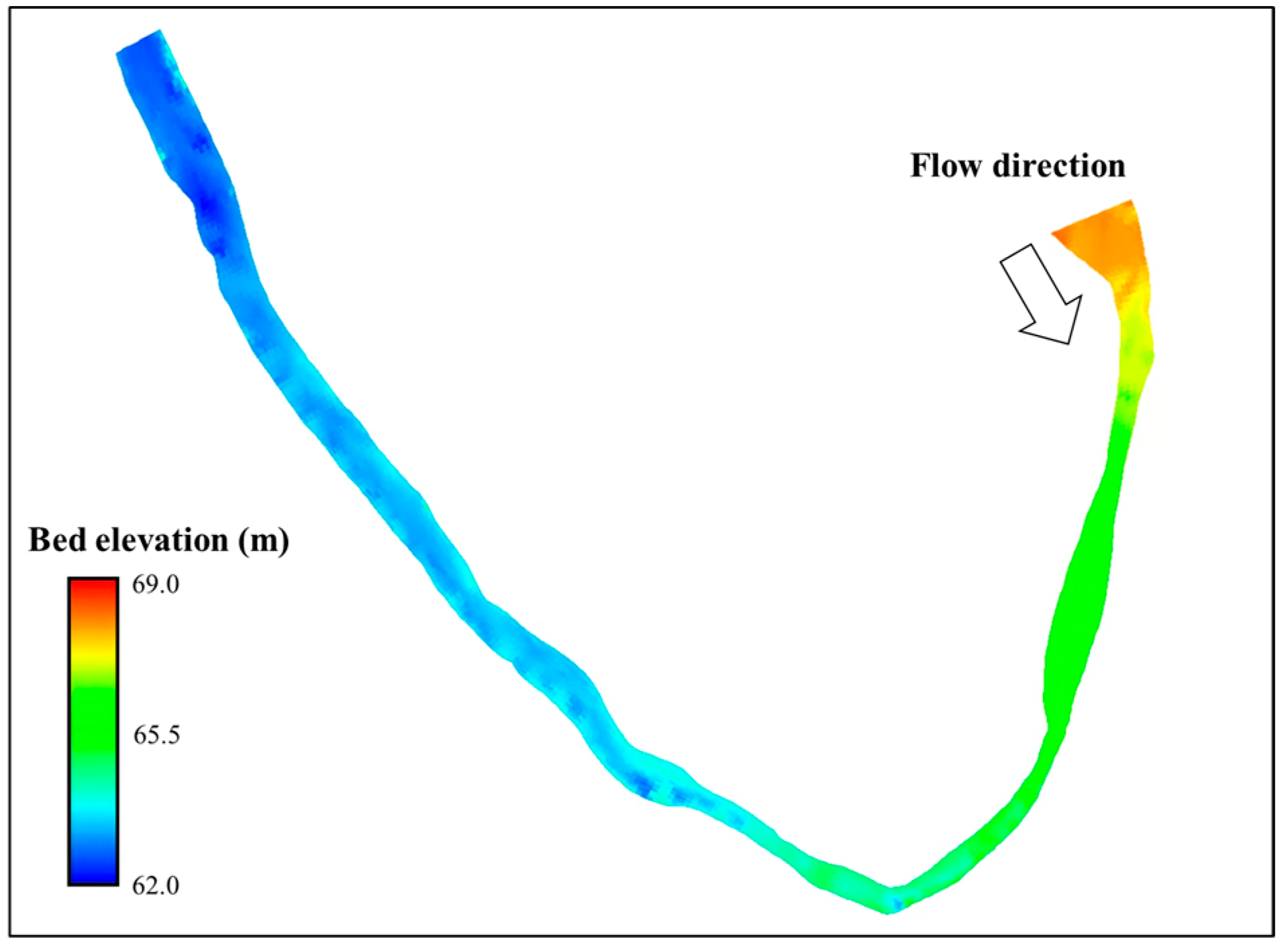
The EFDC model was used to simulate the flow and water depth of the Sum River in comparison to the measured data from the field experiment. The study area was discretized using a curvilinear grid based on the bathymetry from the field measurement, as described in Figure 3, and the model was set up with the boundary conditions and parameters calibrated from the field measurement. The numerical grid was generated with a total of 7330 cells corresponding to the bathymetry of the study area and was built with dx varying from 3 to 10 m and dy varying from 1 to 5 m spatial resolution. For the vertical grid, the sigma coordinate was used assuming the number of vertical layers is the same for the water column regardless of water depth difference. In this study, 10 vertical layers were used. The time step of the simulation was set to 0.1 s, which was set to the Courant number less than 0.4.
The discharge flow rate of 5.9 m3/s and measured water surface elevation of 62.2 El.m were originally used for the boundary conditions of the model. Figure 4 shows comparisons of the simulation by the EFDC model with the measured depth-averaged velocity and water depth data in order to demonstrate the validation of the model. Flow simulation results adequately reproduced the velocity distribution, with the R2 (coefficient of determination) and normalized root mean square error (RMSE/U), which were specifically determined at the measured sections as 0.738 and 0.713; 0.27 and 0.32, respectively, which are acceptable values.
Comparisons of the simulation by the EFDC model with the measured tracer experiment results are displayed in Figure 4. Agreements between the measured tracer data and the EFDC simulation are generally good in the measured sections in Figure 5 with the R2 and normalized RMSE with peak concentration (RMSE/Cpeak), which were specifically determined at the measured sections as 0.600 and 0.952, 0.17, and 0.08, respectively. Agreements between the measured tracer data and the EFDC simulation are generally good in the measured sections. Section 1’s concentration–time curve exhibits symmetric characteristics in the simulation, while the real measured tracer data already have a curve with a longer tail. In the measurements, frictions due to channel irregularities create a long tail based on the non-Fickian mixing properties, where the balance between shear advection and vertical diffusion is incomplete [35]. On the other hand, the simulation results reproduce balanced results between shear advection and vertical diffusion based on the Fickian dispersion. These discrepancies decrease as the balance is accomplished. However, in the recirculation zone between Section 1 and Section 2, solute trapping occurs, creating a long tail in concentration curves. Through these mixing processes, the model exhibits high similarities in Section 2, which is located after the river bend. The model was successful in capturing the effects of the recirculation zone at the bend but had more difficulty in modeling retention effects before the meander in Section 1. After this validation, continuous modeling simulations with different discharge values were conducted using the model to determine the effects of discharge changes on the recirculation zone and contaminant spread.
4. Results
4.1. Occurrence of Recirculation Zone in the Channel Meander
For additional modeling using various discharge data in order to determine its effects on the recirculation zone, the discharge values were increased in increments of 3 m3/s based on continuous simulation, and the results indicated that a significant size increase to the recirculation zone appeared in discharge rates over 9 m3/s. The downstream boundary conditions using water levels for various discharge conditions were based on the measured data from a bridge located downstream from the field experiment site. The bridge had an automatic flow meter using an ADVM (acoustic Doppler velocity meter). Figure 6 compares the measured data from the gauge site with the conventional power function equation , which was created using the measured values before the field experiment was conducted. The stage–discharge equation is in good fit with the measured values in discharge rates below 100 m3/s, which includes the range in this research. Figure 7 shows the simulation results of the 2D velocity contour of case Q = 18 m3/s.
In meandering channels, flow recirculation at the outer bank occurs through rotation along a horizontal, streamwise axis, which shows a separation alongside the main flow. The friction-induced decrease in flow velocity close to the outer bank, which can produce tiny vortices, is what can cause the outer bank cell. Under most flow conditions, the flow velocity close to the outer bank is significantly lower than the flow velocity of the main flow. To find the characteristics and changes to the recirculation pattern at the meander of the natural river, additional modeling simulations using various discharge rates were conducted. The simulation results with streamlines are presented in Figure 8 in UTM coordinates, indicating that the recirculation zone area increased as the discharge increased.
The size of the recirculation zone in Figure 8 in the streamwise and spanwise directions is quantitively depicted in Figure 9. The streamwise direction was defined as the general direction of the bulk flow of the river, which can be seen with the streamlines outside of the recirculation zone. In all cases with increasing discharge, the recirculation zone size did not change significantly for the spanwise direction but increased accordingly in the streamwise direction, as the recirculation zone area increased due to discharge increase. This could indicate that, in meandering channels, higher volumes of water flow could contribute to larger areas of reverse flow in the direction of the river. Also, with higher discharge values, the size increase in the recirculation zone became smaller, which is related to the size of the outer bend in the meandering channel, as the size of the recirculation zone cannot be greater than the size of the outer bend.
4.2. Analysis of the Longitudinal Dispersion Coefficient Affected by the Recirculation Zone
Table 1 lists the skewness values for concentration curves derived from model results at different discharge rates. Skewness is normally a statistical measure that describes the asymmetry of the distribution, and in the case of concentration curves, it explains whether the peak of the distribution is leading or lagging the center of mass of the curve, as shown in Equation (9). In all cases, the skewness increased from Section 1 to Section 2, due to the effect of the recirculation zone located between the sections, which affected the tail of the concentration–time curves. An interesting point is that as the discharge increased, the skewness value tended to decrease in Section 2, which implies that the peak of the concentration curve becomes more symmetrical and centered as the flow rate increases. This could be due to increased mixing and a more uniform velocity profile at higher discharges, which leads to a more evenly distributed tracer plume. Thus, the skewness difference () between Section 1 and Section 2 also decreased with the increase in the flow rate. According to Figure 10, the cross-sectional average concentration–time curves for case Q = 5.9 m3/s imply that when concentration values are displayed relative to the concentration peak, the curves for Section 2 and the center of recirculation have longer tails with higher skewness values.
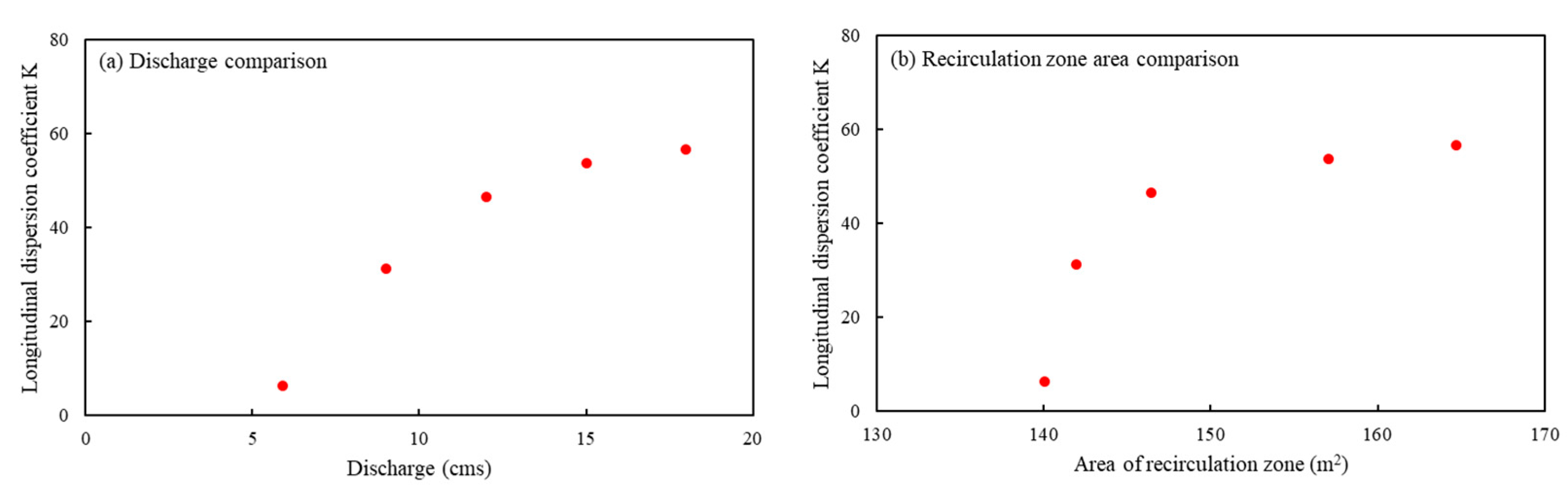
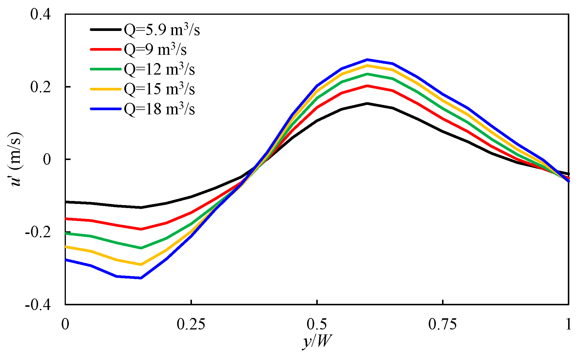
To determine the effect of increased discharge on the longitudinal dispersion coefficient K, the centroid and moments of concentration distribution for the measured sections were calculated for the estimation of K. Figure 11a displays that the values of the longitudinal dispersion coefficient K increase in comparison to the increase in discharge. A scatter plot illustrates the relationship between the longitudinal dispersion coefficient K and the area of the recirculation zone estimated by using the streamlines in Figure 8, where the region of reverse flow separate from that of the main flow is apparent, denoted in square meters (m2) in Figure 11b. As the area of the recirculation zone increased, the longitudinal dispersion coefficient K also tended to increase. This suggests that larger recirculation zones might enhance the mixing of substances within the flow. Another factor involved in the increase in the longitudinal dispersion is the cross-sectional velocity deviation in the transverse direction. Figure 12 depicts the simulated cross-sectional velocity deviation in the transverse direction at the center of the recirculation zone. The intersection points depicted in Figure 12, where y/W ranges from 0.35 to 0.4, are created near the boundary of the recirculation zone. Around the intersection points, the velocity deviation across the channel width increased, and the results indicated that in the recirculation zone, the activation of the shear flow dispersion occurred. Furthermore, the velocity deviation increased even more with an increase in the flow rate. The difference in how higher discharge values resulted in a higher difference between the lower and higher velocity values, which led to higher shear flow, and this could be a reason why the longitudinal dispersion K value increased with higher discharge values.
4.3. Analysis of the Concentration Curves Affected by the Recirculation Zone
The effects of discharge increase on the recirculation zone and contaminant retention were further investigated by calculating the amount of cumulative contaminant passing through the recirculation zone. Figure 13 shows the change in dimensionless dosage depicted at the channel. In higher discharge flows, the total cumulative contaminant passed more through areas not in the recirculation zone, due to a higher relative velocity in the higher discharge model results. This proves that a higher discharge can lead to larger recirculation zones, but the amount of contaminant that is actually being transported into the recirculation zone could decrease since more parts of the contaminant are being transported by the main flow outside the recirculation zone.
Additional analysis was carried out, with the results shown in Figure 14. The graph depicts the variation in the concentration normalized by the peak concentration over time, which was plotted for different discharge values in the recirculation zone. The curves display the normal pattern in concentration–time curves, where the concentration quickly rises to a peak and then gradually declines due to various reasons, one of which is the effect of storage zones. The graph analysis indicates that when the discharge value increased, the time taken to attain the peak concentration decreased. The lowest discharge case took the longest time to reach its peak, while the highest discharge case reached its peak the quickest. This implies that a higher discharge rate leads to a faster transport of the substance at the center of the recirculation zone. After reaching the peak, each curve descends at different rates, with the higher discharge rates generally declining more quickly, which may suggest that the substance stays shorter in the recirculation zone at higher discharge rates. This may possibly be due to the greater momentum generated by higher velocity overcoming the recirculating motion [36], which may retain the contaminant shorter before it is transported out of the zone.
5. Discussion
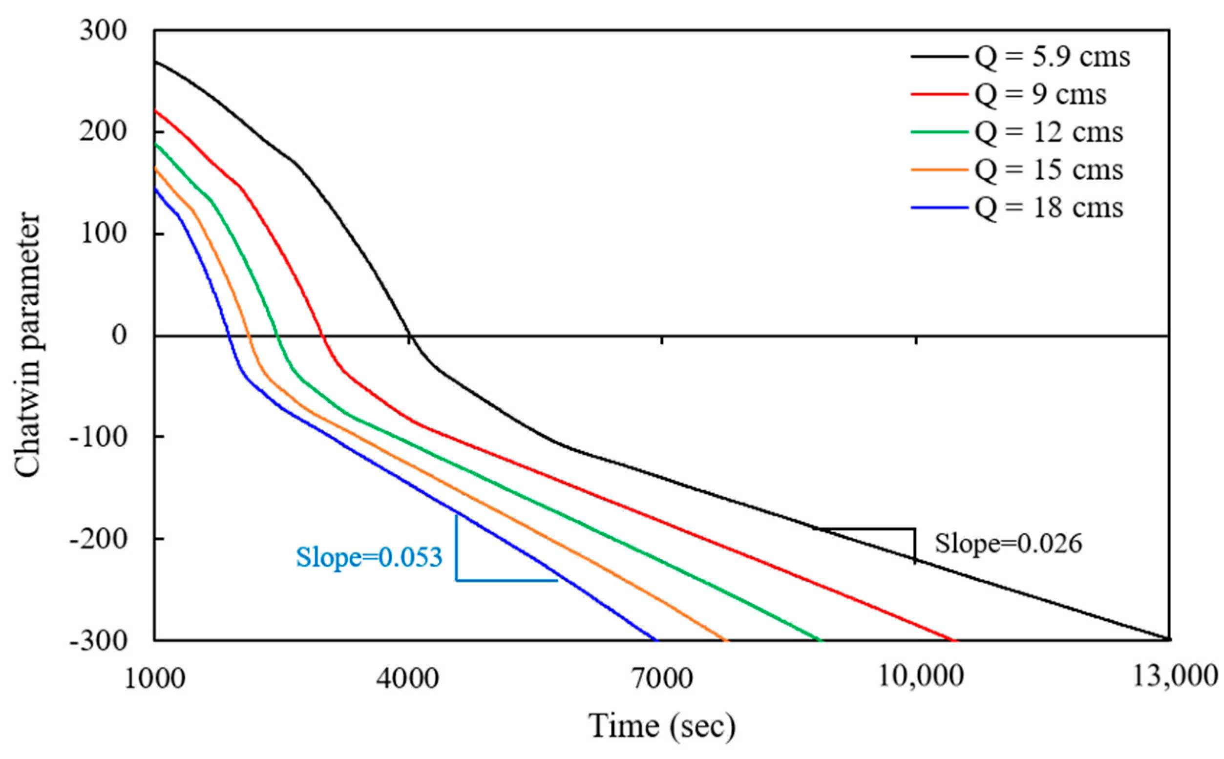
The storage zone generated in the river meander bends generates a long tail on the concentration–time curve [37], affecting the results of the one-dimensional longitudinal dispersion (K) of rivers. However, the recirculation zones generated in the river meander bends influence the three-dimensional flow structure, thus imposing limitations on interpretation using one-dimensional storage zone models. Therefore, we analyzed the influence of storage zones on the cross-sectional average concentration–time curves by using the quasi-three-dimensional simulation results. Additional analysis of the concentration–time curves in Figure 14 was conducted by calculating the Chatwin parameter using the tail part of the concentration–time curves for various discharge rates at the center of a recirculation zone, with the following equation:
where tmax is the time when the maximum concentration (Cmax) occurs. This parameter often relates to the analysis of dispersion in flows, especially in cases of contaminants or tracers in rivers. Figure 15 is the calculation result of Chatwin’s parameter change in time for different discharge rates. The values in the figure decrease over time for all discharge values since it focuses on the time of the concentration tail, but the slope of the values changes according to the differences in discharge cases. The fact that the curves are not parallel indicates that the rate of dispersion, or the size of the trapped concentration due to the storage zone, is not constant across the different discharge values. It is known that the calculated values of Chatwin’s parameter follow a linear line when the concentration–time curve follows the Gaussian distribution. All model results using different discharge display different slopes, indicating that there could be a relationship between the discharge rate and the efficiency of mixing or spreading within the recirculation zone. The slope exhibits the asymmetric characteristics of the tail in the concentration curve, which could allow for the prediction of how long contaminants could remain concentrated in a particular area such as the recirculation zone in the meandering area. The higher slope in Figure 15 with the high discharge demonstrates that higher discharge values result in the tail of the concentration curve becoming shorter.
Figure 11a indicates that the longitudinal dispersion increases with higher flow rates. According to the theoretical interpretation of shear dispersion by Fischer [24], the increase in longitudinal dispersion results from increased velocity deviations across the channel cross-section and reduced transverse dispersion. As depicted in Figure 11a and Figure 12, higher flow rates lead to an increase in velocity deviation, indicating higher shear flow, which leads to an increase in longitudinal dispersion, similar to the theoretical interpretation. Moreover, the enlarged recirculation zone size contributes to reducing transverse dispersion, as evidenced by flatter dosage curves under lower flow rate conditions (Figure 12), consistent with the findings of previous research [10]. These results align with field experimental results [37,38,39], where the longitudinal dispersion coefficient excluding storage zone effects was estimated to be smaller than the K values obtained after incorporating storage zone effects.
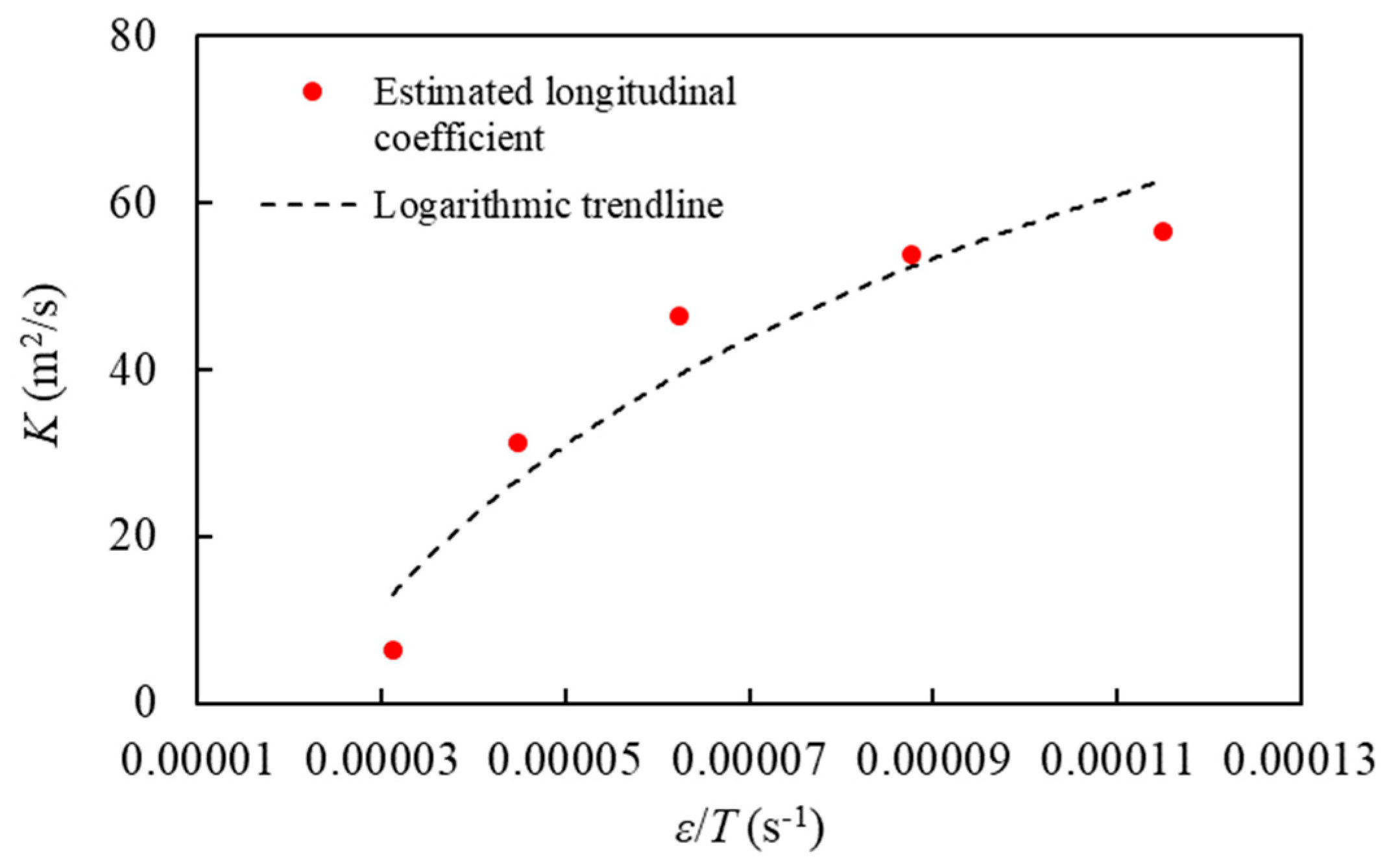
To determine the parameters of the storage zone model ( and ), previous studies have employed the curve-fitting method, which estimates optimal parameters to replicate measured C-t curves [40,41]. The simulation results (Figure 8 and Figure 14) suggest that the storage zone parameters can be directly estimated instead of relying on the curve-fitting method. Figure 16 illustrates the relationship between the mass exchange rate () and K, incorporating the effects of the storage zone. The findings indicate that longitudinal dispersion accelerates with the development of the recirculation zone, accompanied by an increase in the exchange rate coefficient between the flow and the storage zone, . The intensification of recirculation zones due to increased flow rates leads to an elevation in the exchange rate coefficient between the flow and storage zone, fostering active mass exchange between these zones and mitigating contaminant trapping within the storage zone. Consequently, higher flow rates result in the formation of a strong shear plane at the boundary of the recirculation zone, reducing the influx of contaminants into the storage zone and facilitating the rapid transfer of contaminants from the storage zone to the mainstream. As a result, the contaminant trapping effect in the storage zone diminishes, leading to a decrease in transverse dispersion and an increase in the dispersion of contaminants through the flow zone.
6. Conclusions
In this study, the storage zone size changes caused by various discharge rates and how they affected the movement of contaminants were examined by modeling and tracer tests. A field experiment was conducted in a natural river and the measured tracer data were used for the validation of the EFDC model. Through the modeling of storage zones based on different discharge conditions, our research found that the recirculation zone size can increase due to discharge increase. The greater flow rate caused velocity deviation to increase over the cross-section as the recirculation zone increased.
Then, an analysis of the characteristics of the concentration curve by changes in the length and width of the storage zone and a comparison of dispersion coefficient results were performed. The findings demonstrated that because of the greater relative velocity in the model results at higher discharge flows, the total cumulative contaminant could pass more through areas outside the recirculation zone even though the recirculation zone size increased. Moreover, with higher discharge rates, the contaminant spent less time in the recirculation zone. This could potentially be attributed to the increased momentum generated by surpassing the recirculating motion at a higher velocity. The enlarged recirculation zone size can contribute to reducing transverse dispersion, as evidenced by flatter dosage curves under lower flow rate conditions. These findings suggest that the concurrent effects of recirculation zone development, namely a higher velocity deviation across the channel width and a reduction in transverse dispersion, contribute to an increase in longitudinal dispersion. Understanding these dynamics could be valuable for future research in this field.
Author Contributions
Conceptualization, I.P. and J.S.; methodology, S.H.J. and J.S; software, S.H.J.; validation, S.H.J.; writing—original draft preparation, J.S. and I.P.; writing—review and editing, S.H.J., I.P., and J.S.; project administration, I.P. and J.S.; funding acquisition, S.H.J. and J.S. All authors have read and agreed to the published version of the manuscript.
Funding
This work was supported by the Gachon University research fund of 2022 (GCU-202205740001). This work was also funded by the Basic Science Research Program through the National Research Foundation of Korea (NRF), Ministry of Education (2021R1A6A3A01088484).
Data Availability Statement
The data presented in this study are available on request from the corresponding author. The data are not publicly available due to the substantial size of data volume.
Conflicts of Interest
The authors declare no conflicts of interest.
References
- Blanckaert, K.; De Vriend, H.J. Secondary flow in sharp open-channel bends. J. Fluid Mech. 2004, 498, 353–380. [Google Scholar] [CrossRef]
- Blanckaert, K. Flow separation at convex banks in open channels. J. Fluid Mech. 2015, 779, 432–467. [Google Scholar] [CrossRef]
- Ferguson, R.I.; Parsons, D.R.; Lane, S.N.; Hardy, R.J. Flow in meander bends with recirculation at the inner bank. Water Resour. Res. 2003, 39, 1322–1335. [Google Scholar] [CrossRef]
- Blanckaert, K. Hydrodynamic processes in sharp meander bends and their morphological implications. J. Geophys. Res. Earth Surf. 2011, 116, F01003. [Google Scholar] [CrossRef]
- Hu, C.; Yu, M.; Wei, H.; Liu, C. The mechanisms of energy transformation in sharp open-channel bends: Analysis based on experiments in a laboratory flume. J. Hydrol. 2019, 571, 723–739. [Google Scholar] [CrossRef]
- Marion, A.; Zaramella, M. Effects of velocity gradients and secondary flow on the dispersion of solutes in a mean-dering channel. J. Hydraul. Eng. 2006, 132, 1295–1302. [Google Scholar] [CrossRef]
- Kim, J.S.; Seo, I.W.; Baek, D.; Kang, P.K. Recirculating flow-induced anomalous transport in meandering open-channel flows. Adv. Water Resour. 2020, 141, 103603. [Google Scholar] [CrossRef]
- Gooseff, M.N.; LaNier, J.; Haggerty, R.; Kokkeler, K. Determining in-channel (dead zone) transient storage by comparing solute transport in a bedrock channel–alluvial channel sequence, Oregon. Water Resour. Res. 2005, 41, W06014. [Google Scholar] [CrossRef]
- Jackson, T.R.; Haggerty, R.; Apte, S.V.; Coleman, A.; Drost, K.J. Defining and measuring the mean residence time of lateral surface transient storage zones in small streams. Water Resour. Res. 2012, 48, W10501. [Google Scholar] [CrossRef]
- Shin, J.; Rhee, D.; Park, I. Applications of Two-Dimensional Spatial Routing Procedure for Estimating Dispersion Coefficients in Open Channel Flows. Water 2021, 13, 1394. [Google Scholar] [CrossRef]
- O’connor, B.L.; Hondzo, M.; Harvey, J.W. Predictive modeling of transient storage and nutrient uptake: Implications for stream restoration. J. Hydraul. Eng. 2010, 136, 1018–1032. [Google Scholar] [CrossRef]
- Abderrezzak, K.E.K.; Ata, R.; Zaoui, F. One-dimensional numerical modelling of solute transport in streams: The role of longitudinal dispersion coefficient. J. Hydrol. 2015, 527, 978–989. [Google Scholar] [CrossRef]
- Baek, K.O.; Seo, I.W. Routing procedures for observed dispersion coefficients in two-dimensional river mixing. Adv. Water Resour. 2010, 33, 1551–1559. [Google Scholar] [CrossRef]
- Seo, I.W.; Baek, K.O. Estimation of the longitudinal dispersion coefficient using the velocity profile in natural streams. J. Hydraul. Eng. 2004, 130, 227–236. [Google Scholar] [CrossRef]
- Seo, I.W.; Cheong, T.S. Predicting longitudinal dispersion coefficient in natural streams. J. Hydraul. Eng. 1998, 124, 25–32. [Google Scholar] [CrossRef]
- Kim, J.S.; Seo, I.W.; Shin, J.; Jung, S.H.; Yun, S.H. Modeling 2D residence time distributions of pollutants in natural rivers using RAMS+. J. Korea Water Resour. Assoc. 2021, 54, 495–507. [Google Scholar]
- Fisher, H.B. Dispersion predictions in natural streams. J. Sanit. Eng. Div. 1968, 94, 927–943. [Google Scholar] [CrossRef]
- Park, I.; Seo, I.W.; Shin, J.; Song, C.G. Experimental and Numerical Investigations of Spatially-Varying Dispersion Tensors Based on Vertical Velocity Profile and Depth-Averaged Flow Field. Adv. Water Resour. 2020, 142, 103606. [Google Scholar] [CrossRef]
- Yotsukura, N.; Sayre, W.W. Transverse mixing in natural channels. Water Resour. Res. 1976, 12, 695–704. [Google Scholar] [CrossRef]
- Taylor, G.I. The dispersion of matter in turbulent flow through a pipe. Proc. R. Soc. Lond. 1954, 223, 446–468. [Google Scholar] [CrossRef]
- Kashefipour, S.M.; Falconer, R.A. Longitudinal dispersion coefficients in natural channels. Water Res. 2002, 36, 1596–1608. [Google Scholar] [CrossRef]
- Seo, I.W.; Choi, H.J.; Kim, Y.D.; Han, E.J. Analysis of two-dimensional mixing in natural streams based on transient tracer tests. J. Hydraul. Eng. 2016, 142, 04016020. [Google Scholar] [CrossRef]
- Fischer, H.B. Discussion of “simple method for predicting dispersion in streams”. J. Environ. Eng. Div. 1975, 101, 453–455. [Google Scholar] [CrossRef]
- Fischer, H.B.; List, E.J.; Koh, R.C.Y.; Imberger, J.; Brooks, N.H. Mixing in Inland and Coastal Waters, 1st ed.; Academic Press: Cambridge, MA, USA; Elsevier: Amsterdam, The Netherlands, 1979. [Google Scholar]
- Maidment, D.R. Handbook of Hydrology; McGraw-Hill: New York, NY, USA, 1993. [Google Scholar]
- Jackson, T.R.; Haggerty, R.; Apte, S.V. A fluid-mechanics based classification scheme for surface transient storage in riverine environments: Quantitatively separating surface from hyporheic transient storage. Hydrol. Earth Syst. Sci. 2013, 17, 2747–2779. [Google Scholar] [CrossRef]
- Hamrick, J.M. A Three-Dimensional Environmental Fluid Dynamics Computer Code: Theoretical and Computational Aspects; Special Report in Applied Marine Science and Ocean Engineering, No. 317; Virginia Institute of Marine Science: Gloucester Point, VA, USA, 1992; pp. 7–9. [Google Scholar]
- Tong, X.; Mohapatra, S.; Zhang, J.; Tran, N.H.; You, L.; He, Y.; Gin, K.Y.-H. Source, fate, transport and modelling of selected emerging contaminants in the aquatic environment: Current status and future perspectives. Water Res. 2022, 217, 118418. [Google Scholar] [CrossRef] [PubMed]
- Chen, L.; Yang, Y.; Chen, J.; Gao, S.; Qi, S.; Sun, C.; Shen, Z. Spatial-temporal variability and transportation mechanism of polychlorinated biphenyls in the Yangtze River Estuary. Sci. Total Environ. 2017, 598, 12–20. [Google Scholar] [CrossRef] [PubMed]
- Gong, R.; Xu, L.; Wang, D.; Li, H.; Xu, J. Water quality modeling for a typical urban lake based on the EFDC model. Environ. Model. Assess. 2016, 21, 643–655. [Google Scholar] [CrossRef]
- Huang, J.; Qi, L.; Gao, J.; Kim, D.-K. Risk assessment of hazardous materials loading into four large lakes in China: A new hydrodynamic indicator based on EFDC. Ecol. Indic. 2017, 80, 23–30. [Google Scholar] [CrossRef]
- US Environmental Protection Agency. Review of Potential Modeling Tools and Approaches to Support the BEACH Program; US Environmental Protection Agency: Washington, DC, USA, 1999. [Google Scholar]
- SonTek, a Division of YSI Inc. RiverSurveyor S5/M9 System Manual; SonTek, a Division of YSI Inc.: San Diego, CA, USA, 2015. [Google Scholar]
- Rowiński, P.M.; Chrzanowski, M.M. Influence of selected fluorescent dyes on small aquatic organisms. Acta Geophys. 2011, 59, 91–109. [Google Scholar] [CrossRef]
- Park, I.; Seo, I.W. Modeling non-Fickian pollutant mixing in open channel flows using two-dimensional particle dispersion model. Adv. Water Resour. 2018, 111, 105–120. [Google Scholar] [CrossRef]
- Shin, J.; Lee, S.; Park, I. Influences of Momentum Ratio on Transverse Dispersion for Intermediate-Field Mixing Downstream of Channel Confluence. Int. J. Environ. Res. Public Heal. 2023, 20, 2776. [Google Scholar] [CrossRef] [PubMed]
- Nordin, C.F.; Troutman, B.M. Longitudinal dispersion in rivers: The persistence of skewness in observed data. Water Resour. Res. 1980, 16, 123–128. [Google Scholar] [CrossRef]
- Field, M.S.; Pinsky, P.F. A two-region nonequilibrium model for solute transport in solution conduits in karstic aquifers. J. Contam. Hydrol. 2000, 44, 329–351. [Google Scholar] [CrossRef]
- Van Mazijk, A.; Veling, E.J.M. Tracer experiments in the Rhine Basin: Evaluation of the skewness of observed concentration distributions. J. Hydrol. 2005, 307, 60–78. [Google Scholar] [CrossRef]
- Seo, I.W.; Cheong, T.S. Moment-based calculation of parameters for the storage zone model for river dispersion. J. Hydraul. Eng. 2001, 127, 453–465. [Google Scholar] [CrossRef]
- Rodrigues, P.P.G.W.; Gonzalez, Y.M.; de Sousa, E.P.; Neto, F.D.M. Evaluation of dispersion parameters for River Sao Pedro, Brazil, by the simulated annealing method. Inverse Probl. Sci. Eng. 2012, 21, 34–51. [Google Scholar] [CrossRef]
Figure 1.
Storage effects of mixing process at the river meander.

Figure 2.
The study area of Sum River.
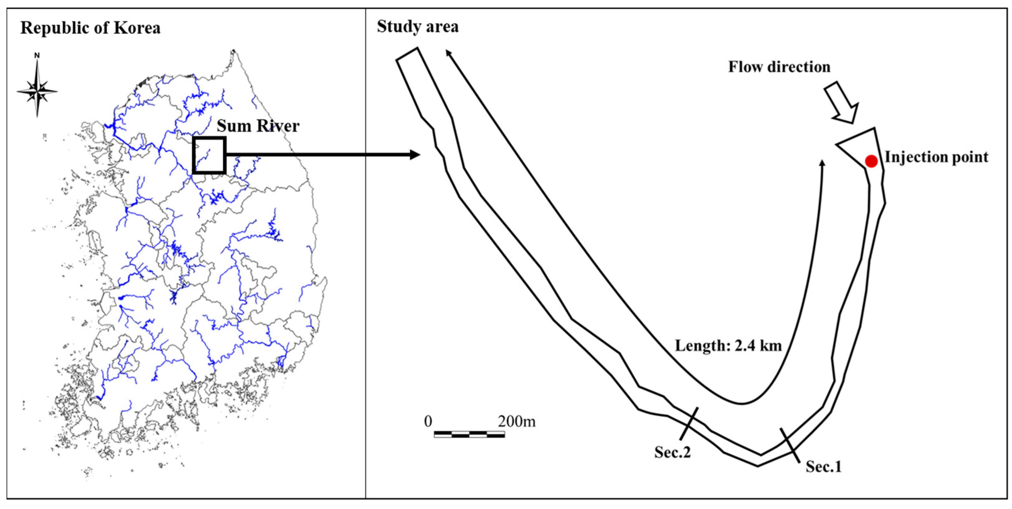
Figure 3.
Topography data with measured bed elevation.

Figure 4.
Comparison of the simulated velocity and water depth profile against measurements: (a) Section 1; (b) Section 2.
Figure 4.
Comparison of the simulated velocity and water depth profile against measurements: (a) Section 1; (b) Section 2.
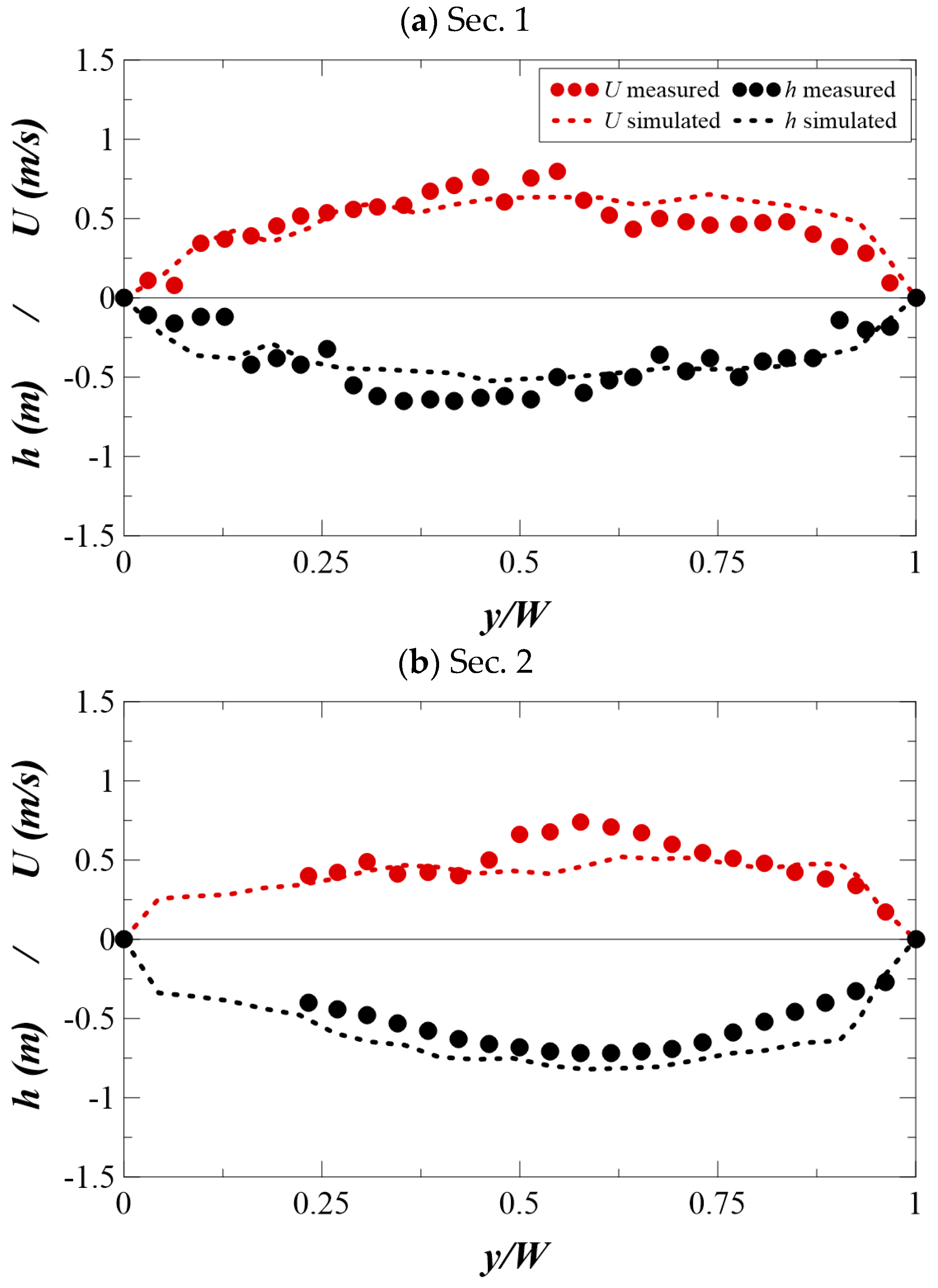
Figure 5.
Comparison of the simulated concentration–time curve against measurement: (a) Section 1; (b) Section 2.
Figure 5.
Comparison of the simulated concentration–time curve against measurement: (a) Section 1; (b) Section 2.

Figure 6.
Comparison of stage–discharge equation and measured values.
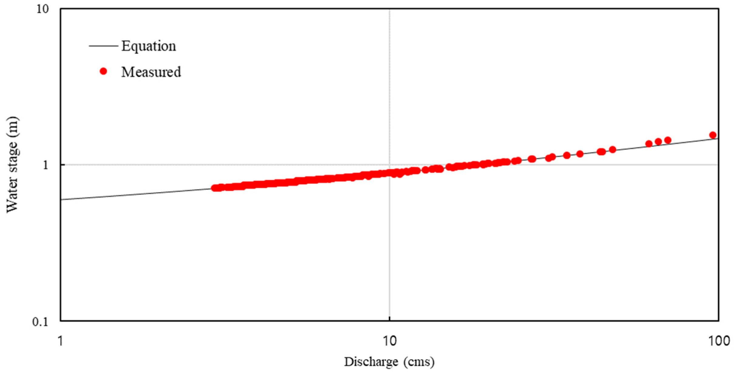
Figure 7.
Simulated velocity field for case Q = 18 m3/s.
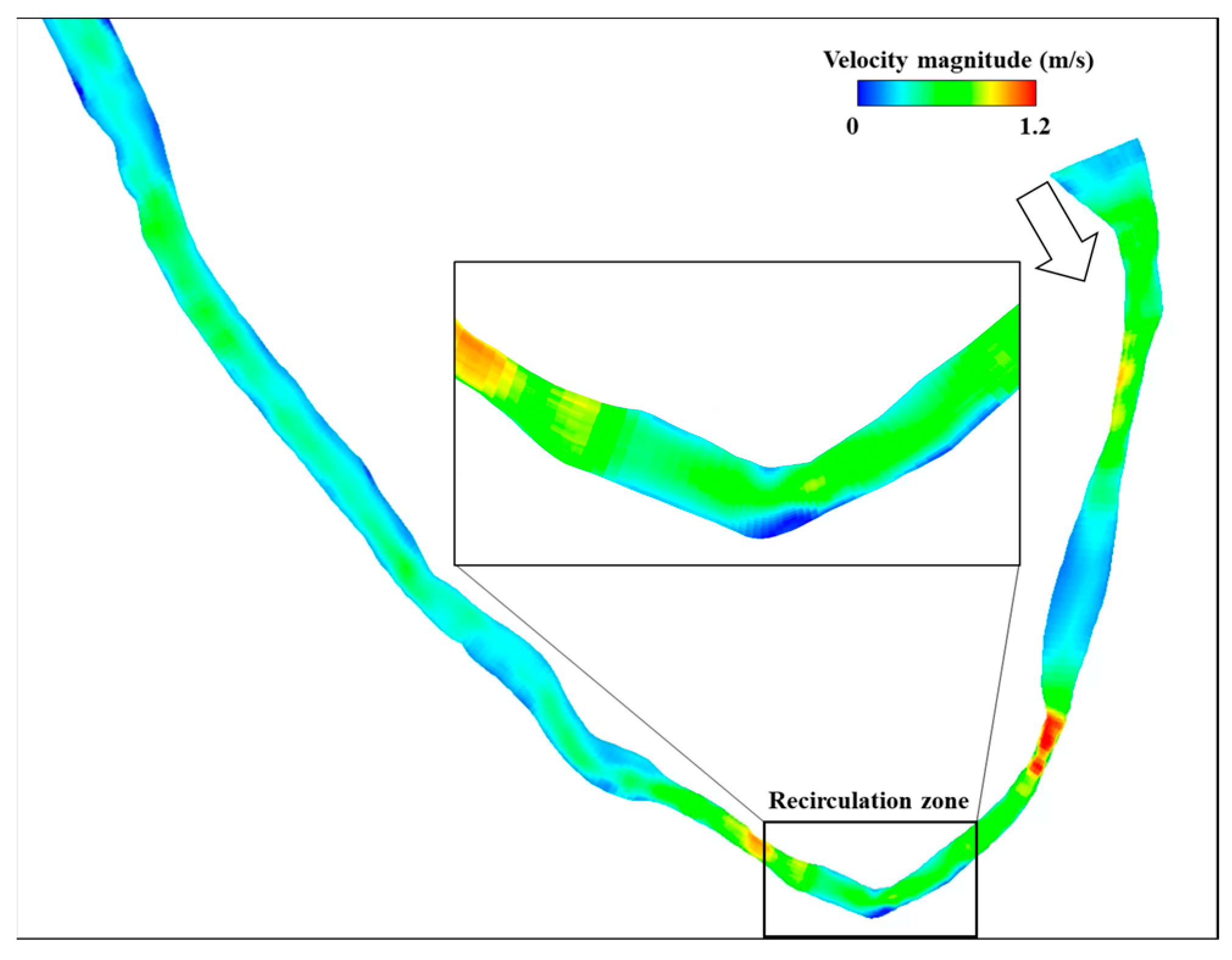
Figure 8.
The recirculation size changes by discharge rate in models with streamlines.
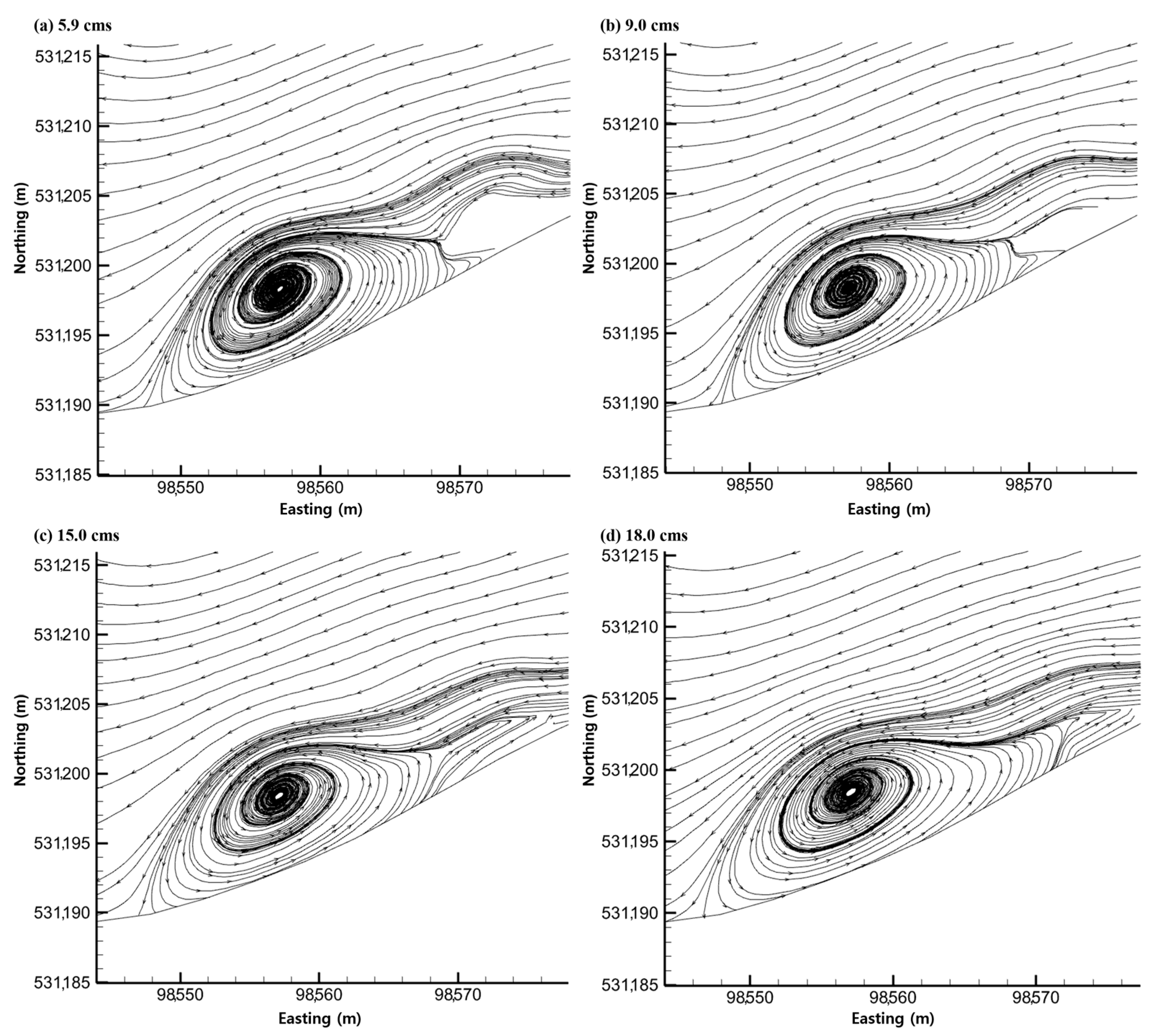
Figure 9.
Relationships between the spanwise and streamwise recirculation zone length and discharge.
Figure 9.
Relationships between the spanwise and streamwise recirculation zone length and discharge.

Figure 10.
Cross-sectional average concentration–time curves for Q = 5.9 m3/s.

Figure 11.
Relationships between the longitudinal dispersion coefficient K and (a) discharge and (b) area of recirculation zone.
Figure 11.
Relationships between the longitudinal dispersion coefficient K and (a) discharge and (b) area of recirculation zone.

Figure 12.
Cross-sectional velocity deviation in the transverse direction at the section with the center of the recirculation zone.
Figure 12.
Cross-sectional velocity deviation in the transverse direction at the section with the center of the recirculation zone.

Figure 13.
Spanwise dimensionless dosage changes starting from the recirculation zone.

Figure 14.
The concentration–time curve changes from the center recirculation zone.
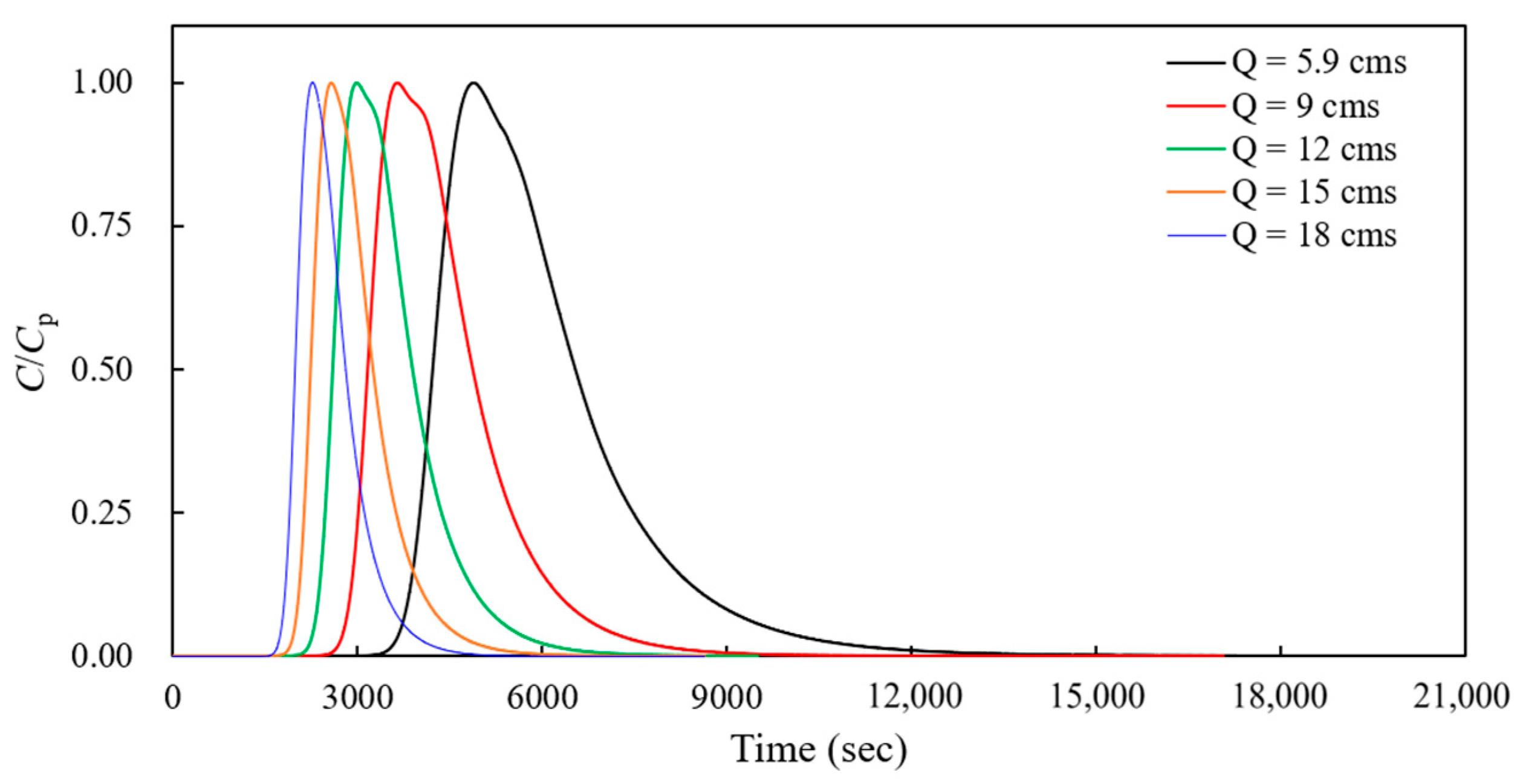
Figure 15.
The Chatwin parameter from concentration–time curves at the center of the recirculation zone.
Figure 15.
The Chatwin parameter from concentration–time curves at the center of the recirculation zone.

Figure 16.
Relationship between the mass exchange rate and the longitudinal dispersion coefficient.

Table 1.
Skewness comparison in Section 1 and Section 2 for all cases.
| Case | R2 | ||
|---|---|---|---|
| Section 1 | Section 2 | ||
| Q = 5.9 m3 | 0.635 | 3.233 | 2.60 |
| Q = 9.0 m3 | 0.626 | 3.035 | 2.41 |
| Q = 12.0 m3 | 0.587 | 2.950 | 2.36 |
| Q = 15.0 m3 | 0.545 | 2.839 | 2.29 |
| Q = 18.0 m3 | 0.508 | 2.712 | 2.20 |
Disclaimer/Publisher’s Note: The statements, opinions and data contained in all publications are solely those of the individual author(s) and contributor(s) and not of MDPI and/or the editor(s). MDPI and/or the editor(s) disclaim responsibility for any injury to people or property resulting from any ideas, methods, instructions or products referred to in the content. |
© 2024 by the authors. Licensee MDPI, Basel, Switzerland. This article is an open access article distributed under the terms and conditions of the Creative Commons Attribution (CC BY) license (https://creativecommons.org/licenses/by/4.0/).
Share and Cite
MDPI and ACS Style
Jung, S.H.; Park, I.; Shin, J. An Investigation of Contaminant Transport and Retention from Storage Zone in Meandering Channels. Water 2024, 16, 1170. https://doi.org/10.3390/w16081170
AMA Style
Jung SH, Park I, Shin J. An Investigation of Contaminant Transport and Retention from Storage Zone in Meandering Channels. Water. 2024; 16(8):1170. https://doi.org/10.3390/w16081170
Chicago/Turabian StyleJung, Sung Hyun, Inhwan Park, and Jaehyun Shin. 2024. "An Investigation of Contaminant Transport and Retention from Storage Zone in Meandering Channels" Water 16, no. 8: 1170. https://doi.org/10.3390/w16081170
Note that from the first issue of 2016, this journal uses article numbers instead of page numbers. See further details here.