Enhancing Smart Irrigation Efficiency: A New WSN-Based Localization Method for Water Conservation

Abstract

The shortage of water stands as a global challenge, prompting considerable focus on the management of water consumption and irrigation. The suggestion is to introduce a smart irrigation system based on wireless sensor networks (WSNs) aimed at minimizing water consumption while maintaining the quality of agricultural crops. In WSNs deployed in smart irrigation, accurately determining the locations of sensor nodes is crucial for efficient monitoring and control. However, in many cases, the exact positions of certain sensor nodes may be unknown. To address this challenge, this paper presents a new localization method for localizing unknown sensor nodes in WSN-based smart irrigation systems using estimated range measurements. The proposed method can accurately determine the positions of unknown nodes, even when they are located at a distance from anchors. It utilizes the Levenberg–Marquardt (LM) optimization algorithm to solve a nonlinear least-squares problem and minimize the error in estimating the unknown node locations. By leveraging the known positions of a subset of sensor nodes and the inexact distance measurements between pairs of nodes, the localization problem is transformed into a nonlinear optimization problem. To validate the effectiveness of the proposed method, extensive simulations and experiments were conducted. The results demonstrate that the proposed method achieves accurate localization of the unknown sensor nodes. Specifically, it achieves 19% and 58% improvement in estimation accuracy when compared to distance vector-hop (DV-Hop) and semidefinite relaxation-LM (SDR-LM) algorithms, respectively. Additionally, the method exhibits robustness against measurement noise and scalability for large-scale networks. Ultimately, integrating the proposed localization method into the smart irrigation system has the potential to achieve approximately 28% reduction in water consumption.

1. Introduction

The global challenge of water scarcity is a pressing issue. Consequently, there is considerable emphasis on water consumption and irrigation management. Conventional agricultural irrigation involves a significant amount of water usage [1]. Hence, there is a growing need to explore smart agriculture approaches designed to diminish water consumption without compromising the quality of agricultural crops. Smart irrigation, driven by advancements in technology, holds great promise for optimizing water consumption and increasing crop productivity. One of the key technologies enabling smart irrigation is wireless sensor networks (WSNs) [2]. These networks comprise spatially distributed sensor nodes that collect and transmit data on environmental conditions such as soil moisture, humidity, and temperature. In the context of smart irrigation systems, WSNs play a crucial role in monitoring and controlling these environmental parameters, facilitating efficient water usage and targeted crop management [3]. WSNs offer several advantages in the domain of smart irrigation. Firstly, they enable real-time and continuous monitoring of environmental variables, allowing farmers to receive decisions concerning irrigation schedules, fertilizer application, and pest management. This data-driven approach enhances precision irrigation practices by enabling tailored interventions at the individual plant level. Secondly, WSNs eliminate the need for manual data collection, reducing labor costs and improving operational efficiency. Additionally, WSNs provide a scalable and cost-effective solution, as they can be deployed over large agricultural areas, covering extensive farmlands [4,5,6].

Accurate localization of sensor nodes within the WSNs is crucial for achieving the desired precision and effectiveness of smart irrigation systems. Node localization is the process of identifying the physical positions of the sensor nodes within the network. Precise node localization enables spatially aware monitoring and control, allowing for targeted actions based on the specific conditions of different areas within the agricultural field [7,8]. For example, localized data on soil moisture levels can be utilized to implement irrigation strategies that precisely deliver water where and when it is needed, minimizing wastage and optimizing plant growth.

The localization of sensor nodes in WSNs has been a subject of extensive research due to its critical role in various applications, including smart irrigation systems. Traditional localization techniques rely on Global Positioning System (GPS) receivers or manual surveying methods, which may not be feasible or economical for large-scale deployments. Moreover, these methods often assume that the positions of all nodes are known or can be accurately measured. However, in practical scenarios, it is common to have a subset of nodes with known positions while the locations of other nodes remain unknown or imprecisely known [9,10].

The problem of localizing unknown nodes in WSNs has garnered significant attention due to its relevance in various applications [11,12,13,14,15,16,17]. In the context of smart agriculture, accurate localization of the unknown nodes allows for complete coverage and spatially aware decision-making. This capability permits precise and controlled water distribution to designated regions within agricultural fields. Through accurate identification of sensor node positions, the system adjusts irrigation strategies in response to real-time data, ensuring targeted water delivery at optimal times and locations. Such localization accuracy effectively minimizes water waste, mitigates the risk of over-irrigation, and facilitates customized irrigation scheduling. By estimating the coordinates of the unknown nodes based on their range measurements to anchor nodes with known positions, the overall network performance can be improved, resulting in more effective resource allocation and optimized irrigation strategies [18].

In this paper, we address the challenge of localizing unknown sensor nodes in WSN-based smart irrigation systems. We propose a new localization method that can minimize the error in node localization. The proposed method utilizes multi-hop localization concept presented in [9] to accurately determine the positions of unknown nodes, even when they are located at a far distance from anchors. The range measurements are derived from the estimated distances between pairs of sensor nodes, typically obtained from received signal strength (RSS) measurements. By formulating the problem as a nonlinear least- squares optimization task, the proposed method leverages the Levenberg–Marquardt (LM) optimization algorithm to reduce the error in estimating the node locations. Through extensive simulations and experiments, we demonstrate the effectiveness and scalability of the proposed method. The results highlight its potential for practical implementation in real-world smart irrigation applications, ultimately contributing to sustainable resource management and increased crop yields.

The motivation behind this research is twofold. Firstly, accurate localization of all sensor nodes enables fine-grained monitoring and control, facilitating precise water allocation and targeted interventions in smart irrigation systems. Secondly, the localization method presented in this paper can be extended to various applications beyond smart irrigation, where the availability of accurate node positions is essential for efficient operation and decision-making. The key contributions of this work can be summarized as follows:

• Proposing a new localization method to localize unknown nodes in WSN-based smart irrigation systems using range measurements and the LM optimization algorithm.
• Demonstrating the effectiveness of the proposed method through extensive simulations and experiments, highlighting accurate node localization amidst measurement noise and even when nodes are situated far from anchors.
• Highlighting the scalability of the proposed method for large-scale networks, showcasing its potential for practical implementation in real-world scenarios.
• Calculating the reduction in water consumption achieved through the implementation of the proposed localization method in the smart irrigation system.

Table 1. Abbreviation list.

Abbreviation	Definition
WSNs	Wireless Sensor Networks
GPS	Global Positioning System
TOA	Time of Arrival
TDOA	Time Difference of Arrival
RSS	Received Signal Strength
ITT	Iterative Triangulation and Trilateration
DV-Hop	Distance Vector-Hop algorithm
LM	Levenberg–Marquardt algorithm
SDR-LM	Semidefinite Relaxation-LM

provides a comprehensive list of the abbreviations and definitions utilized in this paper.

The rest of this paper is structured as follows: Section 2 offers an overview of related work on node localization techniques in WSNs. Section 3 details the proposed method along with problem formulation and the mathematical framework for localizing unknown nodes using range measurements. This section also outlines the steps of the LM optimization algorithm. Section 4 presents the simulation setup and experimental results and discussion. In conclusion, Section 5 summarizes the paper and suggests potential avenues for future research.

2. Related Work

In this section, we provide a summary of the existing literature on node localization techniques in WSNs. Localization plays a crucial role in WSNs by enabling spatial awareness and precise monitoring in various applications, including smart irrigation systems. Numerous methods and algorithms have been proposed to address the node localization problem, aiming to achieve accurate and efficient localization results. We categorize the related work into three main approaches: range-based, range-free, and hybrid localization techniques [19,20,21,22,23,24,25,26,27,28].

Range-based localization techniques rely on distance or range measurements between sensor nodes to estimate their positions [19,20,21,22]. The authors in [19] consider the RSS method for location identification. In [20], an unconventional localization method employing the least-squares method was presented. The localization of target nodes is achieved in [21] through the combined utilization of angle-of-arrival (AOA) and RSS measures. In [22] the authors use time-of-arrival (TOA), time-difference-of-arrival (TDOA), and the Chan algorithm to coordinate the unknown sensors. For instance, the well-known GPS is a range-based localization technique widely used in outdoor environments. However, GPS is not suitable for obstructed environments, making it less practical for smart irrigation systems. Moreover, equipping each sensor node with GPS receivers incurs significant expenses.

Range-free localization techniques, on the other hand, do not rely on distance measurements but instead exploit connectivity information between sensor nodes to estimate their positions [23,24]. One common range-free approach is the centroid algorithm, which calculates the centroid of a set of anchor nodes to estimate the position of a target node [23]. Another range-free method is the distance vector-hop (DV-Hop) algorithm, which utilizes hop-count information and communication range to estimate distances between nodes [24]. These range-free techniques are often computationally efficient but may sacrifice localization accuracy compared to range-based methods.

Hybrid localization techniques aim to combine the strengths of both range-based and range-free approaches to achieve more accurate and robust localization results [25,26]. These methods typically leverage both distance measurements and connectivity information. For instance, the iterative triangulation and trilateration (ITT) algorithm combines triangulation using distance measurements and trilateration using range-free connectivity information [25]. By leveraging the complementary nature of these two approaches, hybrid techniques can improve localization accuracy and overcome the limitations of individual methods [26].

The work in [9] proposes a regularized least-squares multi-hops localization algorithm specifically designed for WSNs. The algorithm aims to improve localization accuracy by incorporating both range-based and range-free localization techniques. The authors recognize the limitations of individual localization methods and propose a hybrid approach that integrates the advantages of range-based and range-free techniques. They introduce a regularization term to the least-squares optimization problem, which helps to mitigate errors and uncertainties in range measurements and connectivity information. By iteratively solving the optimization problem, the algorithm estimates the positions of unknown nodes based on the observed range measurements and connectivity information from neighboring nodes. While the work in [10] focuses on addressing the localization challenge in WSNs, our proposed approach complements this work by specifically targeting the localization of unknown sensor nodes in WSN-based smart irrigation systems. Our method leverages range measurements and the LM method to minimize localization errors and enable accurate positioning of the unknown nodes. Through extensive simulations and experiments, we showcase the effectiveness and scalability of our approach, contributing to the body of knowledge in localization techniques for smart irrigation applications.

While various localization techniques have been proposed for WSNs, few studies specifically address the problem of localizing unknown nodes in the context of smart irrigation systems. The localization methods developed for smart irrigation systems often rely on known anchor nodes with GPS receivers or manual surveys. However, outfitting every sensor node with GPS receivers incurs significant costs. Moreover, in practical scenarios, the locations of some sensor nodes may be unknown or imprecisely known. This presents a unique challenge that requires specialized localization algorithms to estimate the positions of these unknown nodes. In this work, we propose a new method that addresses the challenge of localizing unknown sensor nodes in WSN-based smart irrigation systems. By utilizing range measurements and leveraging the LM optimization algorithm, our method aims to minimize the error in estimating the node locations. Through extensive simulations and experiments, we demonstrate the effectiveness and scalability of the proposed method, showcasing its potential for practical implementation in real-world smart irrigation applications.

In the following section, we present the problem formulation and describe the mathematical framework for our proposed localization method. We then provide details on our approach, emphasizing the utilization of the LM algorithm for accurate node localization.

3. Proposed Localization Method

A smart irrigation system based on WSNs presents a contemporary and forward-thinking approach to achieving efficient and sustainable irrigation practices. This system integrates a network of N sensors strategically positioned within the soil, plants, and environment to monitor and gather crucial data concerning soil moisture, temperature, humidity, rainfall, and other pertinent parameters. Within our WSN, the locations of K sensor nodes are known, while the exact positions of the remaining M = N − K nodes are unknown. Nonetheless, we can overcome this challenge by employing a nonlinear least-squares approach to predict the locations of the unknown M nodes. The locations of these sensor nodes must be determined from the distances to nearby nodes (for example, estimated from the strength of signals received from those nodes).

This section introduces the proposed method for localizing unknown sensor nodes in WSN-based smart irrigation systems using estimated range measurements. The proposed method effectively determines the positions of unknown nodes, even when they are distanced from anchors. The procedures of the proposed method are divided into two stages: the first stage is to formulate distance estimation into a nonlinear least-squares problem. Then, in the second stage, we apply the LM optimization algorithm to address this problem and minimize errors in estimating the unknown node locations. The next two subsections explain these procedures.

3.1. Nonlinear Least-Squares Problem Formulation

The distance measurements can be represented by an undirected graph, as shown in Figure 1. In this figure, the number of vertices in the graph is N. The first M = N − K vertices represent the nodes with unknown positions. These nodes are denoted as the free nodes. The last K vertices are the nodes with known positions and are the anchor nodes.

The node coordinates are denoted as follows:

$$p_1=\left(x_1,y_1\right), p_2=\left(x_2,y_2\right),{\dots ,p}_N=\left(x_N,y_N\right),$$

(1)

In Equation (1), the vectors p₁, …, p_N−K are the unknowns in the problem where the vectors p_N−K+1, …, p_N give the positions of the anchor nodes that are known.

The RSS technique based on the radio propagation path loss model [27,28] is used to estimate the distance between a free node and an anchor node. The RSS in dBm within the log-normal shadow-fading model is expressed as [18]:

$${\mathrm{R}\mathrm{S}\mathrm{S}}_{\mathrm{d}\mathrm{B}\mathrm{m}}\left(d_{nm}\right)=P_{0_{\mathrm{d}\mathrm{B}\mathrm{m}}}\left(d_r\right)-10\gamma {\log }_{10}\left(\frac{d_{nm}}{d_r}\right)-S_{\sigma }$$

(2)

where P₀ represents the RSS at a reference distance d_r, γ is the path loss exponent, d_nm is the true distance between mth free node and nth anchor node, and S_σ denotes the log-normal shadowing effects, which follow a Gaussian distribution with a mean of zero and a variance of σ². Using Equation (2), the estimated distance can be written as:

$${\widehat{d}}_{nm}=d_r{\mathrm{l}\mathrm{o}\mathrm{g}}_{10}^{-1}\left(\frac{P_{0_{\mathrm{d}\mathrm{B}\mathrm{m}}}\left(d_r\right)-{\mathrm{R}\mathrm{S}\mathrm{S}}_{\mathrm{d}\mathrm{B}\mathrm{m}}\left(d_{nm}\right)}{10\gamma }\right)$$

(3)

The edges in Figure 1 indicate the pairs of nodes for which a distance measurement is available. There are L edges, denoted by (i₁, j₁), …, (i_L, j_L). The L distance measurements are given as follows:

$$d_l=‖d_{i_l}{-d}_{j_l}‖+{\epsilon }_l,\hspace{1em}l=1,2,\dots ,L$$

(4)

where ε_l represents the measurement error.

To estimate the location of the free nodes, we minimize the error function as follows:

$${\sum }_{l=1}^L{\left(‖d_{i_l}{-d}_{j_l}‖-d_l\right)}^2={\sum }_{l=1}^L{\left(\sqrt{{\left(x_{i_l}-x_{j_l}\right)}^2+{\left(y_{i_l}{-y}_{j_l}\right)}^2}-d_l\right)}^2$$

(5)

Equation (5) represents a nonlinear least-squares problem with variables x₁, x₂, …, x_N−K and y₁, y₂, …, y_N−K. Thus, we can conclude that our cost function f(u^(l)) is as follows:

$$f\left(u^{\left(l\right)}\right)=\sqrt{{\left(x_{i_l}-x_{j_l}\right)}^2+{\left(y_{i_l}{-y}_{j_l}\right)}^2}-d_l$$

(6)

In Equation (4), we consider the points at the l-th iteration. As a result, utilizing the LM algorithm, we should try to minimize the following:

$${‖f\left(u^{\left(l\right)}\right)+Df\left(u^{\left(l\right)}\right)\left(u-u^{\left(l\right)}\right)‖}^2+{\lambda }^{\left(l\right)}{‖u-u^{\left(l\right)}‖}^2$$

(7)

where D represents the Jacobian matrix, as explained in the next section, and λ is the regularization parameter.

Thus, from our minimizing function in (6) and (7), the unknown positions can be formulated as a nonlinear least-squares problem. The solution of this problem is computed as follows:

$$\widehat{u}=u^{\left(l\right)}-{\left(A^{T}A+{\lambda }^{\left(l\right)}I\right)}^{-1}{A}^{T}f\left(u^{\left(l\right)}\right)$$

(8)

where I represents the identity matrix, (.)^T is the matrix transpose, and $A=Df\left(u^{\left(l\right)}\right)$.

The algorithm will continue to run until the termination condition is satisfied, which is:

$$\nabla g\left(u^{\left(l\right)}\right)=2A^{T}f\left(u^{\left(l\right)}\right)\le {10}^{-5}$$

(9)

3.2. Levenberg–Marquardt Optimization Algorithm

A crucial step in executing the LM algorithm involves the computation of the Jacobian matrix. Recall the definition of the Jacobian matrix, as follows:

$$Df\left(z\right)=\left[\begin{array}{ccc}\begin{array}{cc}\frac{d{f}_1}{d{m}_1}\left(z\right)& \frac{d{f}_1}{d{m}_2}\left(z\right)\\ \frac{d{f}_2}{d{m}_1}\left(z\right)& \frac{d{f}_2}{d{m}_2}\left(z\right)\end{array}& \begin{array}{c}\cdots \\ \cdots \end{array}& \begin{array}{c}\frac{d{f}_1}{d{m}_n}\left(z\right)\\ \frac{d{f}_2}{d{m}_n}\left(z\right)\end{array}\\ \begin{array}{cc}⋮& ⋮\end{array}& \ddots & ⋮\\ \begin{array}{cc}\frac{d{f}_n}{d{m}_1}\left(z\right)& \frac{d{f}_n}{d{m}_2}\left(z\right)\end{array}& \cdots & \frac{d{f}_n}{d{m}_n}\left(z\right)\end{array}\right]$$

(10)

In the considered WSN, m₁, m₂, …, m_n in (10) refer to x₁, x₂, …, x_N−K and y₁, y₂, …, y_N−K, with function f(z) defined in (6). It is clear that the matrix $Df\left(z\right)\in \mathbb{I}{\mathbb{R}}^{\mathrm{L}\times 2(\mathrm{N}-\mathrm{K})}$, as we have a row for each of the L edges, and we have 2(N − K) variables.

Regarding the actual matrix entries themselves, there are four possible derivatives we could require in each row, with the rest of the entries in that row being 0. The four possible derivative expressions are listed in Equation (11):

$$\left[\begin{array}{c}\frac{df\left(u^{\left(l\right)}\right)}{d{x}_{i_l}}\\ \frac{df\left(u^{\left(l\right)}\right)}{d{x}_{j_l}}\\ \begin{array}{c}\frac{df\left(u^{\left(l\right)}\right)}{d{y}_{i_l}}\\ \frac{df\left(u^{\left(l\right)}\right)}{d{y}_{j_l}}\end{array}\end{array}\right]=\left[\begin{array}{c}\frac{\left(x_{i_l}-x_{j_l}\right)}{\sqrt{{\left(x_{i_l}-x_{j_l}\right)}^2+{\left(y_{i_l}{-y}_{j_l}\right)}^2}}\\ \frac{-\left(x_{i_l}-x_{j_l}\right)}{\sqrt{{\left(x_{i_l}-x_{j_l}\right)}^2+{\left(y_{i_l}{-y}_{j_l}\right)}^2}}\\ \begin{array}{c}\frac{\left(y_{i_l}-y_{j_l}\right)}{\sqrt{{\left(x_{i_l}-x_{j_l}\right)}^2+{\left(y_{i_l}{-y}_{j_l}\right)}^2}}\\ \frac{-\left(y_{i_l}-y_{j_l}\right)}{\sqrt{{\left(x_{i_l}-x_{j_l}\right)}^2+{\left(y_{i_l}{-y}_{j_l}\right)}^2}}\end{array}\end{array}\right]$$

(11)

However, we can clearly notice that we have four possible conditions, as follows: both nodes are anchors, one of the two nodes are anchors (either the first node in the edge or the second node), and neither of the two nodes are anchors. In the following, we consider each condition separately.

• If the i-th edge contains nodes that are both anchors, the Jacobian matrix row is all zeros, since both variables are known (assuming points at the l-th iteration):

  $$\nabla f_i{\left(u^{\left(l\right)}\right)}^T=\left[\begin{array}{ccc}0& 0& \begin{array}{cc}\cdots & 0\end{array}\end{array}\right]$$

  (12)
• If the i-th edge contains one anchor node, the Jacobian matrix row will contain the derivatives with respect to the unknown node, with the rest of the entries in that row being 0 (assuming points at the l-th iteration), node 2 as anchor:

  $$\nabla f_i{\left(u^{\left(l\right)}\right)}^T=\left[\begin{array}{ccc}0& 0& \begin{array}{cc}\cdots & \begin{array}{ccc}0& \frac{df\left(u^{\left(l\right)}\right)}{d{x}_{i_l}}& \begin{array}{ccc}0& \cdots & \begin{array}{ccc}0& \frac{df\left(u^{\left(l\right)}\right)}{d{y}_{i_l}}& \begin{array}{ccc}0& \cdots & 0\end{array}\end{array}\end{array}\end{array}\end{array}\end{array}\right]$$

  (13)
• Node 1 as anchor:

  $$\nabla f_i{\left(u^{\left(l\right)}\right)}^T=\left[\begin{array}{ccc}0& 0& \begin{array}{cc}\cdots & \begin{array}{ccc}0& \frac{df\left(u^{\left(l\right)}\right)}{d{x}_{j_l}}& \begin{array}{ccc}0& \cdots & \begin{array}{ccc}0& \frac{df\left(u^{\left(l\right)}\right)}{d{y}_{j_l}}& \begin{array}{ccc}0& \cdots & 0\end{array}\end{array}\end{array}\end{array}\end{array}\end{array}\right]$$

  (14)
• The final condition among the four occurs if the i-th edge contains no anchor nodes, in which our Jacobian matrix row will contain the derivatives with respect to both of the unknown nodes (i.e., a potential of four non-zero elements in the row), all assuming points at the l-th iteration:

  $$\nabla f_i{\left(u^{\left(l\right)}\right)}^T=\left[\begin{array}{ccc}0& \cdots & \begin{array}{cc}\frac{df\left(u^{\left(l\right)}\right)}{d{x}_{i_l}}& \begin{array}{ccc}\cdots & \frac{df\left(u^{\left(l\right)}\right)}{d{x}_{j_l}}& \begin{array}{ccc}\cdots & \frac{df\left(u^{\left(l\right)}\right)}{d{y}_{i_l}}& \begin{array}{ccc}\cdots & \frac{df\left(u^{\left(l\right)}\right)}{d{y}_{j_l}}& \begin{array}{cc}\cdots & 0\end{array}\end{array}\end{array}\end{array}\end{array}\end{array}\right]$$

  (15)

The Levenberg–Marquardt algorithm steps can be summarized as follows:

• Step 1: In each iteration of the algorithm, we first compute $f\left(u^{\left(l\right)}\right)$, and then the Jacobian matrix $Df\left(u^{\left(l\right)}\right)$ row by row, with each row being evaluated for one of the four conditions described above.
• Step 2: Next, within the iteration, the code computes both $‖\nabla g\left(u\right)‖$ and $\widehat{u}$, in order to evaluate $f\left(\widehat{u}\right)$ in comparison with $f\left(u^{\left(l\right)}\right)$. Depending on this calculation, the algorithm updates u^(l+1) and λ^(l+1) as follows:

  $$u^{\left(l+1\right)}=\left\{\begin{array}{l}\widehat{u}, if {‖f\left(\widehat{u}\right)‖}^2<{‖f\left(u^{\left(l\right)}\right)‖}^2\\ u^{\left(l\right)}, otherwise\end{array}\right.$$

  (16)

  $${\lambda }^{\left(l+1\right)}=\left\{\begin{array}{l}{\beta }_1{\lambda }^{\left(l\right)} if {‖f\left(\widehat{u}\right)‖}^2<{‖f\left(u^{\left(l\right)}\right)‖}^2\\ {\beta }_2{\lambda }^{\left(l\right)}, otherwise\end{array}\right.$$

  (17)
• Step 3: If $\nabla g\left(u^{\left(l\right)}\right)=2A^{T}f\left(u^{\left(l\right)}\right)\le {10}^{-5}$, then the algorithm will terminate out of the loop and return the calculated estimated coordinates of the unknown sensor nodes.
• Step 4: If the condition in step 3 is not satisfied, go to step 1. The following flow chart summarizes the proposed method steps and is indicated by Figure 2.

4. Results and Discussion

In this section, MATLAB (R2022b) programming is used to execute the proposed method to predict the estimated coordinates of the unknown sensor nodes in the considered WSN. The algorithm will continue to run until the termination condition, $\nabla g\left(u^{\left(l\right)}\right)\le {10}^{-5}$, is satisfied. The first input argument N is the number of nodes in the network, and it varies according to the considered network scale. This includes K = 9 anchor nodes, positioned as in Figure 1. The N − 9 free nodes are placed randomly in a square area with size 100 × 100 m². Two nodes are connected by an edge if their distance is less than or equal to normalized R. Figure 1 presents an example with N = 30 and the node communication range, R = 40 m. The first output argument E is an L × 2 array, specifying the L edges. The two entries of row l are i_l and j_l, the nodes connected by edge l. The output argument is an N × 2 array with the coordinates of the N nodes. Typical values of β₁ and β₂ are β₁ = 0.8 and β₂ = 2.

Table 2. Simulation parameters.

Parameter	Value
Simulation area	100 × 100 m2
Number of nodes, N	N = 50 for small-scale network
	N = 100 for medium-scale network
	N = 200 for large-scale network
Number of anchor nodes, K	9
R	40 m
Path loss exponent, γ	3
Reference distance dr	1 m
P0	−30.45 dBm
Variance, σ2	5 dB
β1	0.8
β2	2

summarizes the simulation parameters.

4.1. Effect of Network Scale

In this subsection, we study the effects of network scale on the performance of the proposed method.

4.1.1. Small-Scale Network

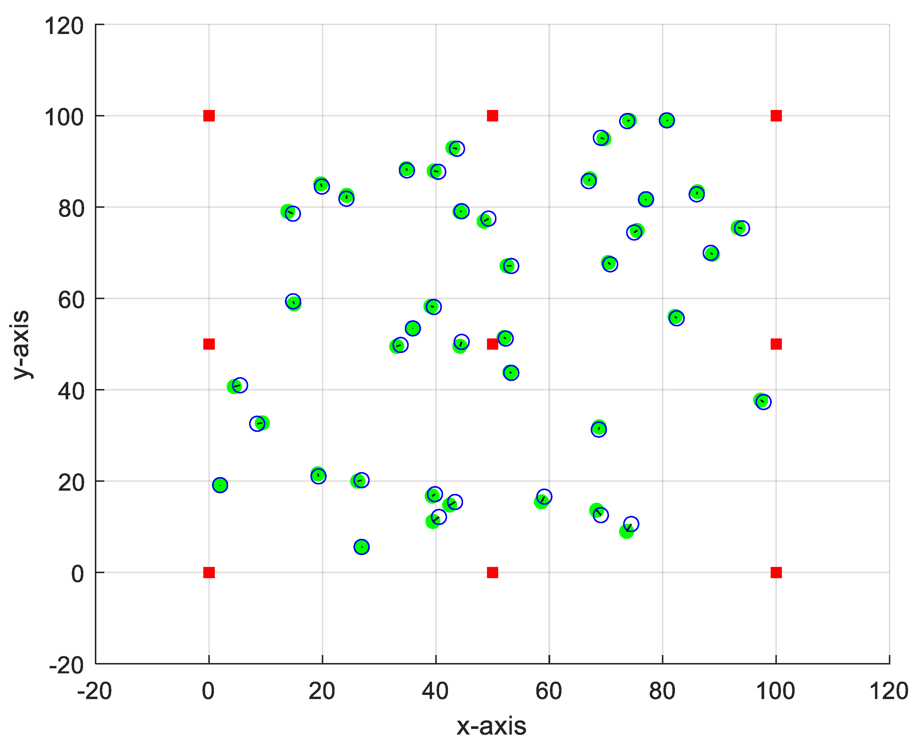
We consider a small-scale network with N = 50 nodes, 9 of them are anchor nodes with known and fixed locations as follows: [(0, 0), (50, 0), (100, 0), (0, 50), (50, 50), (100, 50), (0, 100), (50, 100), (100, 100)]. The free 41 nodes are placed randomly in a square area with size 100 × 100 m². Figure 3 presents the estimation of the sensor coordinate using the proposed method. The open circles (blue) are the exact positions, while the filled circles (green) are the estimated positions. This figure indicates the accuracy of the proposed method in estimating the unknown location of the free nodes.

4.1.2. Medium-Scale Network

In this part, we check the accuracy of the proposed method when increasing the number of network nodes to N =100 nodes. For fair comparison, we use 9 anchor nodes at the same location as in the small-scale case, i.e., there are 91 unknown free nodes. Figure 4 shows the estimated positions versus the exact positions, considering a medium-scale network (N = 100). This figure indicates the accuracy of the proposed method, even for a large number of free nodes.

4.1.3. Large-Scale Network

Now we consider a large-scale network with N = 200 nodes, as shown in Figure 5. The obtained result in this figure ensures the ability of the proposed method to accurately estimate the position of the free nodes, even for a large-scale network.

Figure 6 presents the cost function versus number of iterations for the three network scenarios. As expected, the large-scale network requires the largest cost function compared to the other networks.

4.2. Effect of Changing the Anchor Node Locations

In this subsection, we study the effect of changing the position of the anchor nodes on the accuracy of position estimation using the proposed method. The 9 anchor nodes new location is located around the network center, as follows: [(20, 20), (50, 20), (80, 20), (20, 50), (50, 50), (80, 50), (20, 80), (50, 80), (80, 80)].

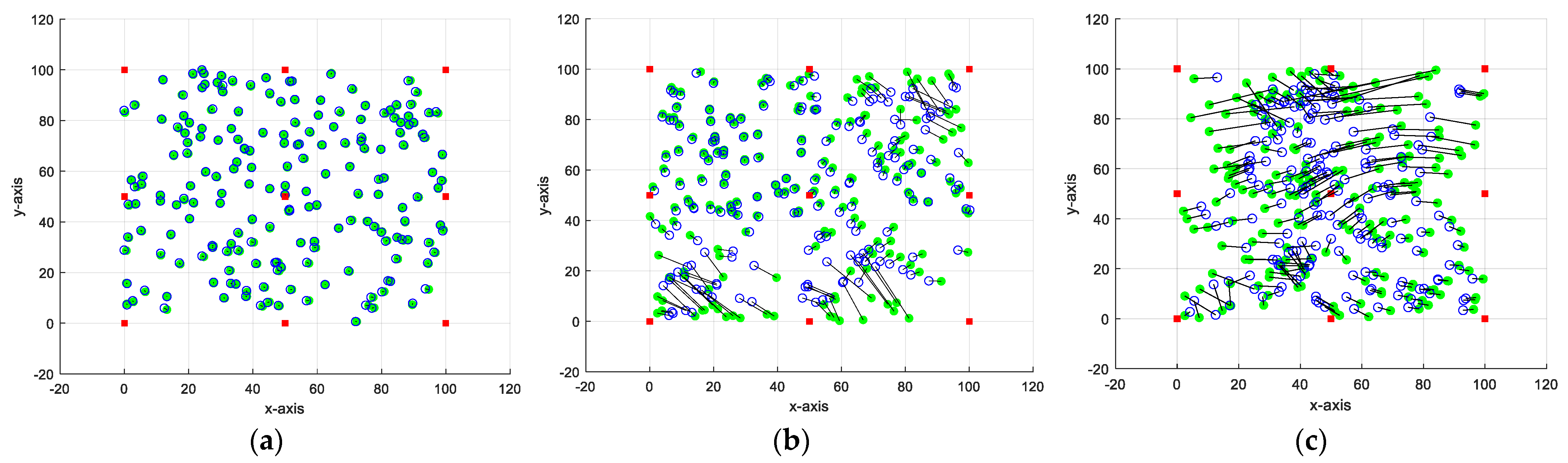
Figure 7 presents the least-squares estimate of the sensor coordinate using the three network scenarios considered above, i.e., N = 50 (a), 100 (b), and 200 (c). This figure indicates that the accuracy of the proposed method is affected by changing the anchor node’s location. However, the reduction in estimation accuracy is small, which ensures the robustness of the proposed method. The anchor node’s new location is around the network center; therefore, its accuracy becomes less than that at network boundaries. This figure also shows that as the number of free nodes increases from 50 to 200, the proposed method’s estimation accuracy decreases.

4.3. Performance Comparison

In this subsection we compare the performance of the proposed method with other localization algorithms presented in the literature, such as improvement of the DV-Hop algorithm [9] and SDR+LM algorithm [9]. For fair comparison, we use the average localization error (ALE) presented in [10] and given as:

$$\mathrm{A}\mathrm{L}\mathrm{E}={\sum }_{i=1}^{N-K}\sqrt{\frac{{\left({\widehat{x}}_i-x_i\right)}^2+{\left({\widehat{y}}_i-y_i\right)}^2}{N-K}}$$

(18)

where N − K represents the number of free nodes (unknown position nodes), $\left(x_i,{xy}_i\right) \mathrm{a}\mathrm{n}\mathrm{d} ({\widehat{x}}_i,{\widehat{y}}_i)$ are the exact and the estimated locations, respectively of node i.

Figure 8 presents a comparison between the proposed method and the algorithms presented in [9,10] using the above-mentioned parameters and the large-scale network case. As explained above, the open circles (blue) are the exact positions, while the filled circles (green) are the estimated positions, and the black straight line that connects between the two circle types represents the positioning error. This figure indicates that the proposed method achieves the lowest localization error when compared to the other algorithms.

In Figure 9, we study the effect of changing the number of anchor nodes on the accuracy of the location estimation of the proposed method. We consider the case of N = 200 nodes and R = 40. This figure presents the ALE versus the number of anchor nodes for the proposed method and the localization algorithms cited above [9,10].

The depicted figure illustrates a clear trend wherein the ALE diminishes with an increase in the number of anchor nodes. This observation can be attributed to the deliberate augmentation of anchor nodes within the network, while keeping the total number of nodes constant. This augmentation is intended to reduce the hop count between the anchors and unknown nodes. As a result, the estimated distance between an anchor and an unknown node more accurately corresponds to the actual distance, leading to a decrease in the average positioning error. Additionally, the figure demonstrates that the proposed method yields a lower localization error compared to all other algorithms considered in the comparison. At a number of anchor nodes of 9, the proposed method achieves 19% and 58% improvement in estimation accuracy, respectively, when compared to the above-cited localization algorithms [9,10]. Where these algorithms estimate the positions of unknown nodes based on the observed range measurements and connectivity information from neighboring nodes, this reduces the estimation accuracy and increases the computational accuracy of these algorithms, while the proposed method is based on the LM estimation algorithm, which is more accurate than range-free localization algorithms.

4.4. Water Consumption Calculation

Accurate sensor node localization is integral to the efficient functioning of a smart irrigation system and plays a crucial role in optimizing water consumption. In a smart irrigation network based on WSNs, precise knowledge of sensor node locations enables targeted and controlled water distribution to specific areas of agricultural fields. By accurately determining the positions of sensor nodes, the system can adapt irrigation strategies based on real-time data, ensuring that water is delivered precisely where and when it is needed. This localization precision minimizes water wastage, prevents over-irrigation, and allows for the implementation of tailored irrigation schedules. Consequently, the synergy between accurate sensor node localization and water consumption in a smart irrigation system leads to improved resource efficiency, reduced environmental impact, and sustainable agricultural practices. Due to the accuracy achieved by the proposed method, it is expected that smart irrigation with the proposed method can reduce the amount of water consumption when compared to other methods.

The efficacy of irrigation relies on monitoring environmental conditions and plant requirements. This is due to the fact that plant water requirements are influenced by factors such as temperature, moisture levels, precipitation, and soil moisture. The values of these factors depend mainly on the accuracy of sensor node localization. Therefore, it is expected that the implementation of the smart irrigation system using the proposed method will result in a reduction in water consumption compared to alternative methods.

Figure 10 illustrates a comparison among the methods examined in this paper concerning water consumption during one day for a small-scale network [1,29,30]. In this figure, we considered a pump with a capacity of 50 liters per hour, and the conventional irrigation system requires one hour for irrigation; therefore, it consumes 50 liters. On the other hand, the smart irrigation methods function four times a day, according to Figure 6 presented in [30], with different irrigation times, according to the considered method, as presented in

Table 3. Irrigation time and consumed water for the considered irrigation methods.

Irrigation Method	Irrigation Time	Consumed Water
Conventional irrigation	60 min	50,000 mL
Smart irrigation using DV-Hop algorithm [9]	4 × 12 min = 48 min	40,000 mL
Smart irrigation using SDR+LM algorithm [10]	4 × 12.9 min = 51.6 min	43,000 mL
Smart irrigation without using localization method [30]	4 × 13.2 min = 52.8 min	44,000 mL
Smart irrigation using proposed method	4 × 10.8 min = 43.2 min	36,000 mL

[1,29,30]. The analysis of the data was conducted utilizing SAS software [1] which determined the irrigation time for each irrigation method. This time represents the time during which the irrigation valve was on, according to the sensor reading.

As depicted in Figure 10, it becomes evident that the smart irrigation system employing the proposed method can substantially diminish the volume of water consumed in comparison to alternative methods. Specifically, it attains an impressive 28% reduction in irrigation water consumption when compared with the conventional irrigation technique. The accurate estimation of the sensor node positions ensures the delivery of water precisely where and when it is needed. In contrast, smart irrigation systems utilizing the DV-Hop algorithm [9], the SDR+LM algorithm [10], and the smart irrigation system without using localization method in [30] achieve approximately 20%, 14%, and 12% reductions, respectively, in the amount of water consumed when compared to the conventional irrigation technique.

5. Conclusions

This paper addressed the challenge of localizing unknown sensor nodes in WSN-based smart irrigation systems, underscoring the pivotal role of accurate node localization for efficient monitoring and control. The proposed method, leveraging range measurements and the Levenberg–Marquardt optimization algorithm, emerged as a robust solution, minimizing errors in estimating the unknown node locations. Quantitative analysis revealed compelling results, showcasing the proposed method’s superior performance. Specifically, it achieved an impressive 19% and 58% enhancement in estimation accuracy compared to DV-Hop and SDR+LM localization algorithms, respectively. Extensive simulations and experiments across various network scales demonstrated not only the accuracy but also the scalability of the method, affirming its effectiveness even in large-scale scenarios. The numerical results unequivocally establish that the proposed method significantly improves estimation accuracy, substantiating its superiority over existing localization methods. This research provides concrete evidence of the method’s potential, emphasizing its practical applicability and potential for achieving a substantial 28% reduction in water consumption in smart irrigation systems where the accurate estimation of sensor node positions ensures the delivery of water precisely where and when it is needed.

Future research includes exploring the influence of environmental factors on localization accuracy, integrating additional sensing modalities for enhanced precision, investigating scalability for larger networks, and developing energy-efficient algorithms to prolong network lifespan.

References

- Sharifnasab, H.; Mahrokh, A.; Dehghanisanij, H.; Łazuka, E.; Łagód, G.; Karami, H. Evaluating the Use of Intelligent Irrigation Systems Based on the IoT in Grain Corn Irrigation. Water 2023, 15, 1394. [Google Scholar] [CrossRef]
- Deepa, R.; Sankar, M.; R, R.; Sankari, C.; Venkatasubramanian; Kalaivani, R. IoT based Energy Efficient using Wireless Sensor Network Application to Smart Irrigation. In Proceedings of the 2023 International Conference on Intelligent Data Communication Technologies and Internet of Things (IDCIoT), Bengaluru, India, 5–7 January 2023; pp. 90–95. [Google Scholar] [CrossRef]
- Hassan, E.S. Energy-Efficient Resource Allocation Algorithm for CR-WSN-Based Smart Irrigation System under Realistic Scenarios. Agriculture 2023, 13, 1149. [Google Scholar] [CrossRef]
- Shanmugasundaram, N.; Kumar, G.S.; Sankaralingam, S.; Vishal, S.; Kamaleswaran, N. Smart Irrigation Using Modern Technologies. In Proceedings of the 2023 9th International Conference on Advanced Computing and Communication Systems (ICACCS), Coimbatore, India, 17–18 March 2023; pp. 2025–2030. [Google Scholar] [CrossRef]
- Pagano, A.; Croce, D.; Tinnirello, I.; Vitale, G. A Survey on LoRa for Smart Agriculture: Current Trends and Future Perspectives. IEEE Internet Things J. 2023, 10, 3664–3679. [Google Scholar] [CrossRef]
- Shaikh, F.K.; Karim, S.; Zeadally, S.; Nebhen, J. Recent Trends in Internet-of-Things-Enabled Sensor Technologies for Smart Agriculture. IEEE Internet Things J. 2022, 9, 23583–23598. [Google Scholar] [CrossRef]
- Zhu, Y.; Yan, F.; Zhao, S.; Xing, S.; Shen, L. On improving the cooperative localization performance for IoT WSNs. Ad Hoc Netw. 2021, 118, 102504. [Google Scholar] [CrossRef]
- Singh, P.; Singh, P.; Mittal, N.; Singh, U.; Singh, S. An optimum localization approach using hybrid TSNMRA in 2D WSNs. Comput. Netw. 2023, 226, 109682. [Google Scholar] [CrossRef]
- Liouane, H.; Messous, S.; Cheikhrouhou, O.; Baz, M.; Hamam, H. Regularized Least Square Multi-Hops Localization Algorithm for Wireless Sensor Networks. IEEE Access 2021, 9, 136406–136418. [Google Scholar] [CrossRef]
- El Badawy, D.; Larsson, V.; Pollefeys, M.; Dokmanić, I. Localizing Unsynchronized Sensors With Unknown Sources. IEEE Trans. Signal Process. 2023, 71, 641–654. [Google Scholar] [CrossRef]
- Zhao, X.; Zhang, X.; Sun, Z.; Wang, P. New Wireless Sensor Network Localization Algorithm for Outdoor Adventure. IEEE Access 2018, 6, 13191–13199. [Google Scholar] [CrossRef]
- Khan, A.U.; Khan, M.E.; Hasan, M.; Zakri, W.; Alhazmi, W.; Islam, T. An Efficient Wireless Sensor Network Based on the ESP-MESH Protocol for Indoor and Outdoor Air Quality Monitoring. Sustainability 2022, 14, 16630. [Google Scholar] [CrossRef]
- Alam, S.; Shuaib, M.; Ahmad, S.; Jayakody, D.N.K.; Muthanna, A.; Bharany, S.; Elgendy, I.A. Blockchain-Based Solutions Supporting Reliable Healthcare for Fog Computing and Internet of Medical Things (IoMT) Integration. Sustainability 2022, 14, 15312. [Google Scholar] [CrossRef]
- Hakami, N.A.; Mahmoud, H.A.H.; AlArfaj, A.A. An Intelligent Tracking System for Moving Objects in Dynamic Environments. Actuators 2022, 11, 274. [Google Scholar] [CrossRef]
- Alharbi, F.; Zakariah, M.; Alshahrani, R.; Albakri, A.; Viriyasitavat, W.; Alghamdi, A.A. Intelligent Transportation Using Wireless Sensor Networks Blockchain and License Plate Recognition. Sensors 2023, 23, 2670. [Google Scholar] [CrossRef] [PubMed]
- Bharany, S.; Sharma, S.; Frnda, J.; Shuaib, M.; Khalid, M.I.; Hussain, S.; Iqbal, J.; Ullah, S.S. Wildfire Monitoring Based on Energy Efficient Clustering Approach for FANETS. Drones 2022, 6, 193. [Google Scholar] [CrossRef]
- Prashar, D.; Rashid, M.; Siddiqui, S.T.; Kumar, D.; Nagpal, A.; AlGhamdi, A.S.; Alshamrani, S.S. SDSWSN—A Secure Approach for a Hop-Based Localization Algorithm Using a Digital Signature in the Wireless Sensor Network. Electronics 2021, 10, 3074. [Google Scholar] [CrossRef]
- Annepu, V.; Sona, D.R.; Ravikumar, C.V.; Bagadi, K.; Alibakhshikenari, M.; Althuwayb, A.A.; Alali, B.; Virdee, B.S.; Pau, G.; Dayoub, I.; et al. Review on Unmanned Aerial Vehicle Assisted Sensor Node Localization in Wireless Networks: Soft Computing Approaches. IEEE Access 2022, 10, 132875–132894. [Google Scholar] [CrossRef]
- Mei, X.; Han, D.; Saeed, N.; Wu, H.; Miao, F.; Xian, J.; Chen, X.; Han, B. Navigating the depths: A stratification-aware coarse-to-fine received signal strength-based localization for internet of underwater things. Front. Mar. Sci. 2023, 10. [Google Scholar] [CrossRef]
- Mei, X.; Han, D.; Chen, Y.; Wu, H.; Ma, T. Target localization using information fusion in WSNs-based Marine search and rescue. Alex. Eng. J. 2023, 68, 227–238. [Google Scholar] [CrossRef]
- Mei, X.; Han, D.; Saeed, N.; Wu, H.; Ma, T.; Xian, J. Range Difference-Based Target Localization Under Stratification Effect and NLOS Bias in UWSNs. IEEE Wirel. Commun. Lett. 2022, 11, 2080–2084. [Google Scholar] [CrossRef]
- Lakshmi, Y.V.; Singh, P.; Abouhawwash, M.; Mahajan, S.; Pandit, A.K.; Ahmed, A.B. Improved Chan Algorithm Based Optimum UWB Sensor Node Localization Using Hybrid Particle Swarm Optimization. IEEE Access 2022, 10, 32546–32565. [Google Scholar] [CrossRef]
- Hai, L.; Yang, Z.; Cao, Z.; Yaug, M. An improved weighted centroid localization algorithm based on Zigbee. In Proceedings of the 2022 5th International Conference on Advanced Electronic Materials, Computers and Software Engineering (AEMCSE), Wuhan, China, 22–24 April 2022; pp. 634–637. [Google Scholar] [CrossRef]
- Chen, B.; Guo, X.; Huang, Y.; Yang, M. Improved DV-Hop Node location Optimization Algorithm Based on Adaptive Particle Swarm. In Proceedings of the 2021 2nd International Conference on Artificial Intelligence and Computer Engineering (ICAICE), Hangzhou, China, 5–7 November 2021; pp. 11–17. [Google Scholar] [CrossRef]
- Safavi, S.; Khan, U.A.; Kar, S.; Moura, J.M.F. Distributed Localization: A Linear Theory. Proc. IEEE 2018, 106, 1204–1223. [Google Scholar] [CrossRef]
- Bochem, A.; Zhang, H. Robustness Enhanced Sensor Assisted Monte Carlo Localization for Wireless Sensor Networks and the Internet of Things. IEEE Access 2022, 10, 33408–33420. [Google Scholar] [CrossRef]
- Maddumabandara, A.; Leung, H.; Liu, M. Experimental Evaluation of Indoor Localization Using Wireless Sensor Networks. IEEE Sens. J. 2015, 15, 5228–5237. [Google Scholar] [CrossRef]
- Mei, X.; Chen, Y.; Xu, X.; Wu, H. RSS Localization Using Multistep Linearization in the Presence of Unknown Path Loss Exponent. IEEE Sens. Lett. 2022, 6, 1–4. [Google Scholar] [CrossRef]
- Zia, H.; Rehman, A.; Harris, N.R.; Fatima, S.; Khurram, M. An Experimental Comparison of IoT-Based and Traditional Irrigation Scheduling on a Flood-Irrigated Subtropical Lemon Farm. Sensors 2021, 21, 4175. [Google Scholar] [CrossRef]
- Naji, A.Z.; Salman, A.M. Water Saving in Agriculture through the Use of Smart Irrigation System. In Proceedings of the DSDE ‘21: 2021 4th International Conference on Data Storage and Data Engineering, Barcelona, Spain, 18–20 February 2021; pp. 153–160. [Google Scholar] [CrossRef]
Figure 1.
Network model example with 9 anchor nodes (squares), 21 free nodes (circles), and 98 edges.
Figure 2.
Flow chart of the proposed method.
Figure 3.
Least-squares estimate of the sensor coordinate using N = 50.
Figure 4.
Least-squares estimate of the sensor coordinate using N = 100.
Figure 5.
Least-squares estimate of the sensor coordinate using N = 200.
Figure 6.
Cost function versus number of iterations for 3 network scenarios.
Figure 7.
Effect of changing the position of anchor nodes on the accuracy of the proposed method. (a) N = 50; (b) N = 100; (c) N = 200.
Figure 8.
Performance comparison between the proposed method (a), DV-Hop algorithm [9] (b), and SDR+LM algorithm [10] (c).
Figure 9.
ALE versus number of anchor nodes for the proposed method and the localization algorithms [9,10].
Figure 10.
Water consumption comparison between the proposed method and the localization algorithms [9,10,30].