
Comparison of Water Quality Prediction for Red Tilapia Aquaculture in an Outdoor Recirculation System Using Deep Learning and a Hybrid Model

Abstract
:1. Introduction
2. Materials and Methods
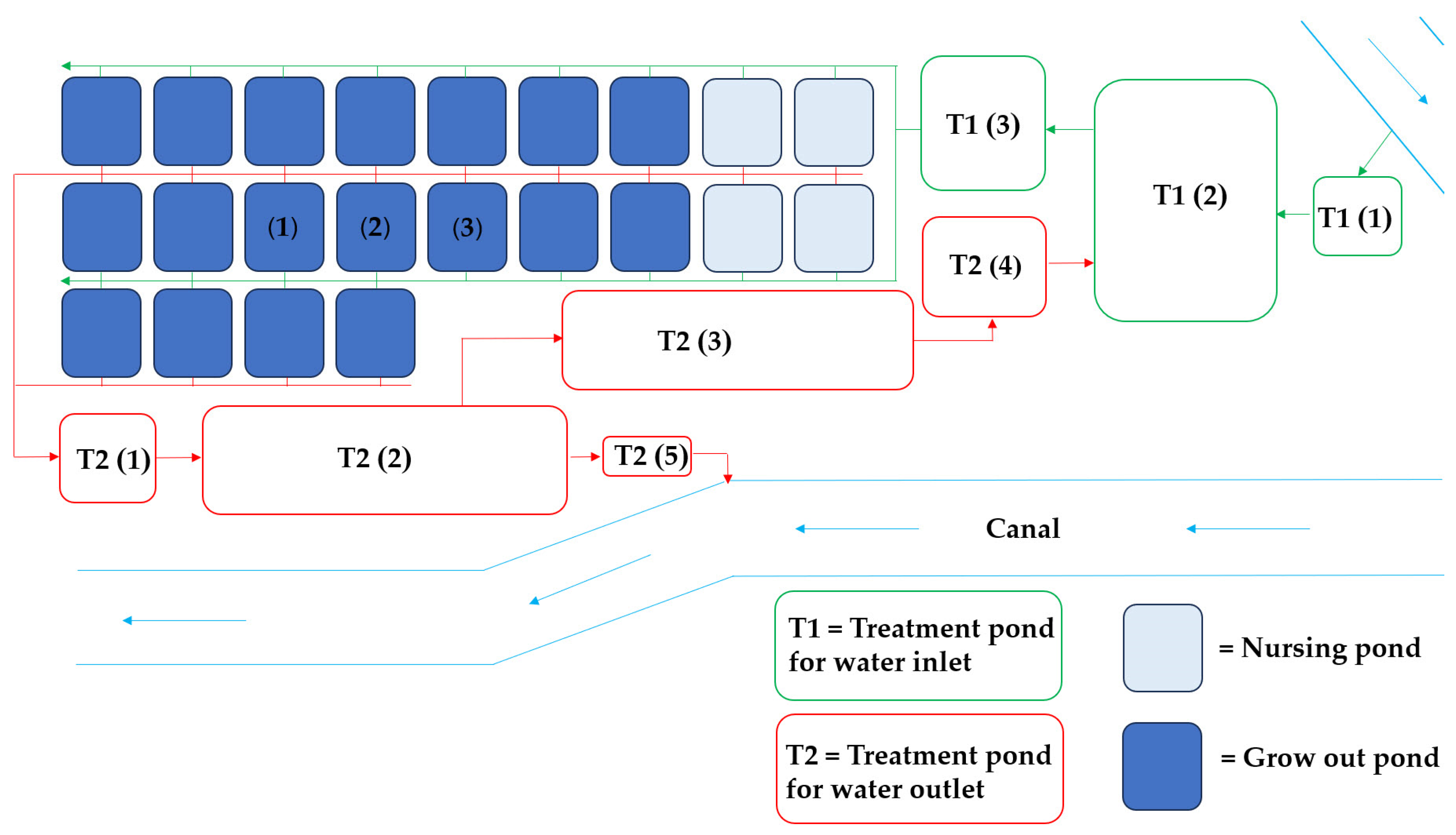
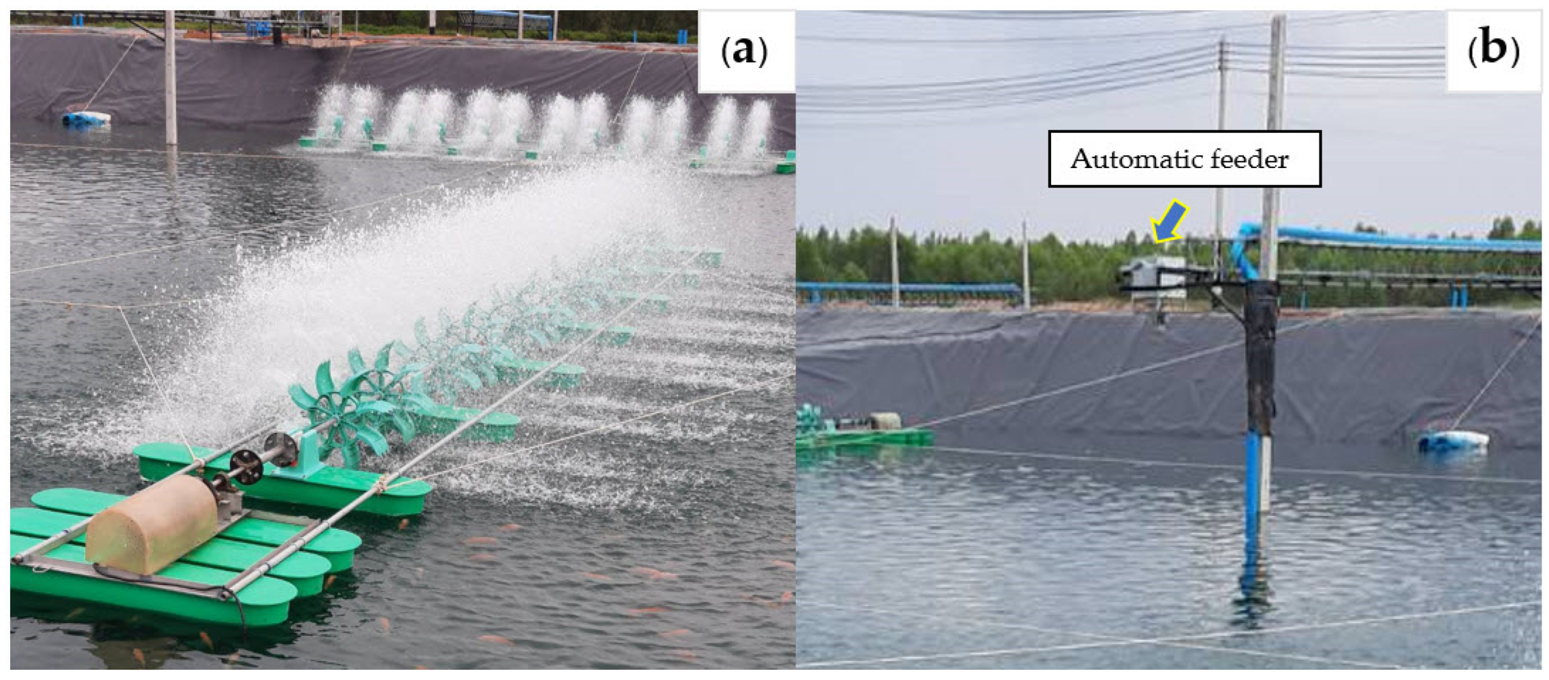
2.1. Farming System and Data Collection
2.2. Water Quality Measurement
2.3. Pre-Processing Dataset
2.4. Feature Selection
2.5. Data Processing, Analysis, and Visualization
2.6. Performance Metrics
2.7. Ethical Statement
3. Results
3.1. Water Quality
3.2. Important Features for Each Water Quality Parameter Prediction
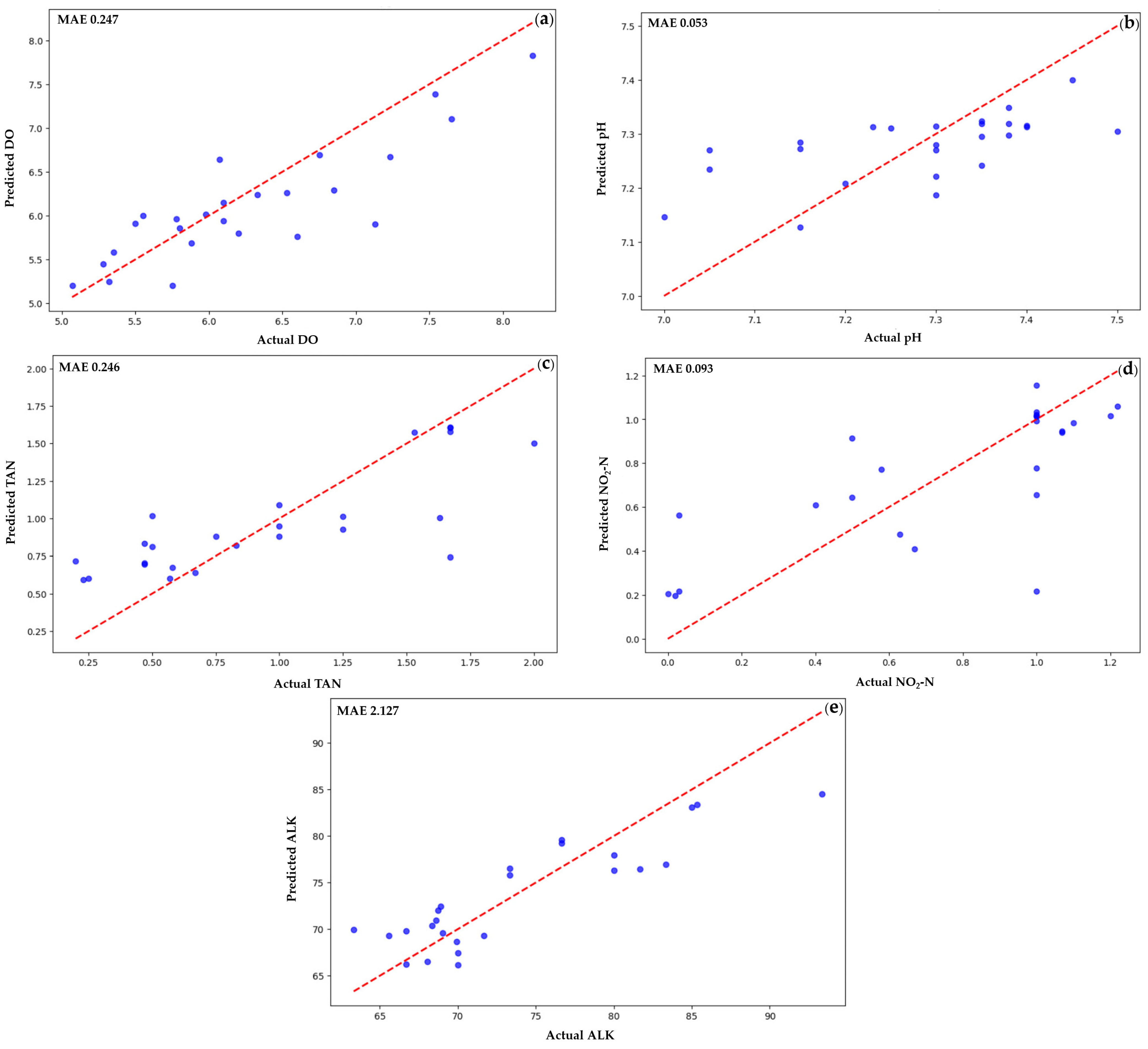
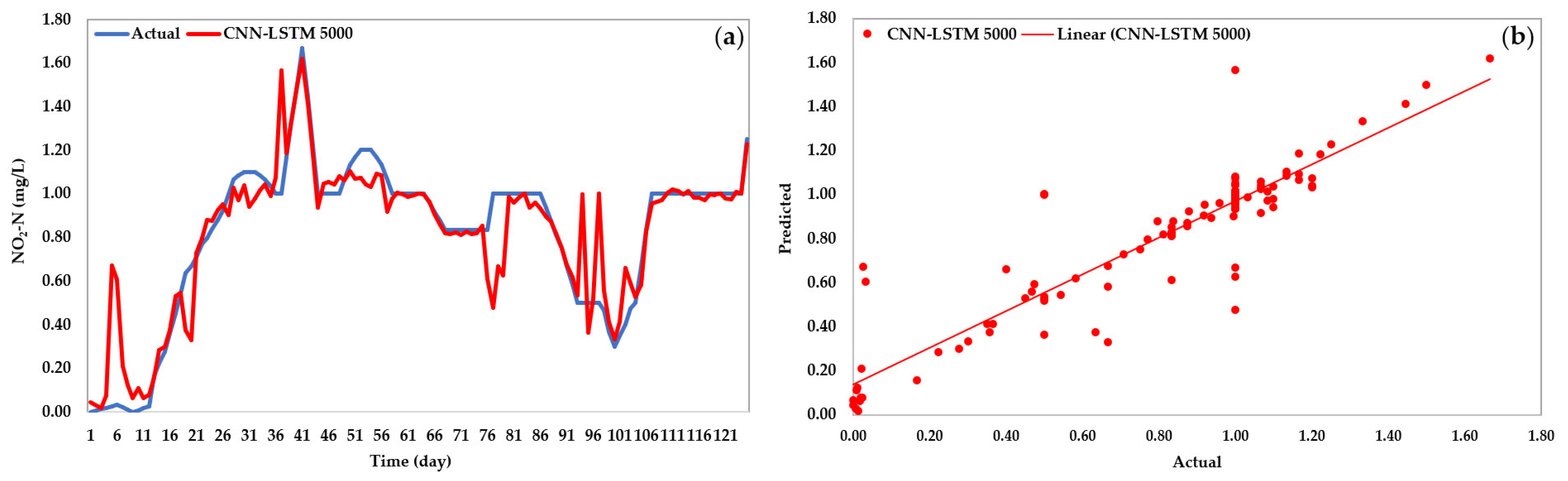
3.3. Predictive Efficiency
4. Discussion
5. Conclusions
Author Contributions
Funding
Data Availability Statement
Acknowledgments
Conflicts of Interest
References
- Amin, M.; Musdalifah, L.; Ali, M. Growth performances of Nile Tilapia, Oreochromis niloticus, reared in recirculating aquaculture and active suspension systems. IOP Conf. Ser. Earth Environ. Sci. 2020, 441, 012135. [Google Scholar] [CrossRef]
- Dalsgaard, J.; Lund, I.; Thorarinsdottir, R.; Drengstig, A.; Arvonen, K. Farming different species in RAS in NORDIC countries: Current status and future perspectives. Aquac. Eng. 2002, 53, 2–13. [Google Scholar] [CrossRef]
- El-Sayed, A.F.M. Effect of stocking density and feeding levels on growth and feed efficiency of Nile tilapia (Oreochrmis niloticus L.) fry. Aquac. Res. 2022, 33, 621–626. [Google Scholar] [CrossRef]
- Gibtan, A.; Getahun, A.; Mengistou, S. Effect of stocking density on the growth performance and yield of Nile tilapia (Oreochromis niloticus L., 1758) in a cage culture system in Lake Kuriftu, Ethiopia. Aquac. Res. 2008, 39, 1450–1460. [Google Scholar] [CrossRef]
- Daudpota, A.M.; Kalhoro, I.B.; Shah, S.A.; Kalhoro, H.; Abbas, G. Effect of stocking densities on growth, production and survival rate of red tilapia in hapa at fish hatchery Chilya Thatta, Sindh, Pakistan. J. Fish. 2014, 2, 180–186. [Google Scholar] [CrossRef]
- Gao, G.; Xiao, K.; Chen, M. An intelligent IoT-based control and traceability system to forecast and maintain water quality in freshwater fish farms. Comput. Electron. Agric. 2019, 166, 105013. [Google Scholar] [CrossRef]
- Ani, J.S.; Manyala, J.O.; Masese, F.O.; Fitzsimmons, K. Effect of stocking density on growth performance of monosex Nile Tilapia (Oreochromis niloticus) in the aquaponic system integrated with lettuce (Lactuca sativa). Aquac. Fish. 2022, 7, 328–335. [Google Scholar] [CrossRef]
- Zambrano, A.F.; Giraldo, L.F.; Quimbayo, J.; Medina, B.; Castillo, E. Machine learning for manually-measured water quality prediction in fish farming. PLoS ONE 2021, 16, E0256380. [Google Scholar] [CrossRef]
- Palani, S.; Liong, S.Y.; Tkalich, P. An ANN application for water quality forecasting. Mar. Pollut. Bull. 2008, 56, 1586–1597. [Google Scholar] [CrossRef]
- Castrillo, M.; López García, A. Estimation of high frequency nutrient concentrations from water quality surrogates using machine learning methods. Water Res. 2020, 172, 115490. [Google Scholar] [CrossRef]
- Anand, M.V.; Sohitha, C.; Saraswathi, G.N.; Lavanya, G.V. Water quality prediction using CNN. J. Phys. Conf. Ser. 2023, 2428, 012051. [Google Scholar] [CrossRef]
- Ye, B.; Cao, X.; Liu, H.; Wang, Y.; Tang, B.; Chen, C.; Chen, Q. Water chemical oxygen demand prediction model based on the CNN and ultraviolet-visible spectroscopy. Front. Environ. Sci. 2022, 10, 1027693. [Google Scholar] [CrossRef]
- Hu, Z.; Zhang, Y.; Zhao, Y.; Xie, M.; Zhong, J.; Tu, Z.; Liu, J. A water quality prediction method based on the Deep LSTM network considering correlation in smart mariculture. Sensors 2019, 19, 1420. [Google Scholar] [CrossRef]
- Liu, P.; Wang, J.; Sangaiah, A.K.; Xie, Y.; Yin, X. Analysis and prediction of water quality using LSTM deep neural networks in IoT environment. Sustainability 2019, 11, 2058. [Google Scholar] [CrossRef]
- Ahmed, U.; Mumtaz, R.; Anwar, H.; Shah, A.A.; Irfan, R.; García-Nieto, J. Efficient water quality prediction using supervised machine learning. Water 2019, 11, 2210. [Google Scholar] [CrossRef]
- Juna, A.; Umer, M.; Sadiq, S.; Karamti, H.; Eshmawi, A.A.; Mohamed, A.; Ashraf, I. Water quality prediction using KNN imputer and multilayer perceptron. Water 2022, 14, 2592. [Google Scholar] [CrossRef]
- Li, T.; Lu, J.; Wu, J.; Zhang, Z.; Chen, L. Predicting aquaculture water quality using machine learning approaches. Water 2022, 14, 2836. [Google Scholar] [CrossRef]
- Wang, X.; Li, Y.; Qiao, Q.; Tavares, A.; Liang, Y. Water quality prediction based on machine learning and comprehensive weighting methods. Entropy 2023, 25, 1186. [Google Scholar] [CrossRef] [PubMed]
- Cojbasic, S.; Dmitrasinovic, S.; Kostic, M.; Sekulic, M.T.; Radonic, J.; Dodig, A.; Stojkovic, M. Application of machine learning in river water quality management: A review. Water Sci. Technol. 2023, 88, 2297–2308. [Google Scholar] [CrossRef]
- da Silva, L.F.B.A.; Yang, Z.; Pires, N.M.M.; Dong, T.; Teien, H.C.; Storebakken, T.; Salbu, B. Monitoring aquaculture water quality: Design of an early warning sensor with Aliivibrio fischeri and predictive models. Sensors 2018, 18, 2848. [Google Scholar] [CrossRef] [PubMed]
- Chen, F.; Du, Y.; Qiu, T.; Xu, Z.; Zhou, L.; Xu, J.; Sun, M.; Li, Y.; Sun, J. Design of an intelligent variable-flow recirculating aquaculture system based on machine learning methods. Appl. Sci. 2021, 11, 6545. [Google Scholar] [CrossRef]
- Yang, J.; Jia, L.; Guo, Z.; Shen, Y.; Li, X.; Mou, Z.; Yu, K.; Lin, J.C.W. Prediction and control of water quality in Recirculating Aquaculture System based on hybrid neural network. Eng. Appl. Artif. Intell. 2023, 121, 106002. [Google Scholar] [CrossRef]
- Wu, J.; Wang, Z. A hybrid model for water quality prediction based on an artificial neural network, wavelet transform, and long short-term memory. Water 2022, 14, 610. [Google Scholar] [CrossRef]
- Zhou, S.; Song, C.; Zhang, J.; Chang, W.; Hou, W.; Yang, L. A hybrid prediction framework for water quality with integrated W-ARIMA-GRU and LightGBM methods. Water 2022, 14, 1322. [Google Scholar] [CrossRef]
- Chen, H.; Yang, J.; Fu, X.; Zheng, Q.; Song, X.; Fu, Z.; Wang, J.; Liang, Y.; Yin, H.; Liu, Z.; et al. Water quality prediction based on LSTM and attention mechanism: A case study of the Burnett River, Australia. Sustainability 2022, 14, 13231. [Google Scholar] [CrossRef]
- Cai, H.; Zhang, C.; Xu, J.; Wang, F.; Xiao, L.; Huang, S.; Zhang, Y. Water quality prediction based on the KF-LSTM encoder-decoder network: A case study with missing data collection. Water 2023, 15, 2542. [Google Scholar] [CrossRef]
- Farzana, S.Z.; Paudyal, D.R.; Chadalavada, S.; Alam, M.J. Prediction of water quality in reservoirs: A comparative assessment of machine learning and deep learning approaches in the case of Toowoomba, Queensland, Australia. Geosciences 2023, 13, 293. [Google Scholar] [CrossRef]
- APHA. Standard Methods for the Examination of Water and Wastewater, 20th ed.; American Public Health Association, American Water Works Association, Water Environment Federation: Washington, DC, USA, 2005. [Google Scholar]
- Kolding, J.; Haug, L.; Stefansson, S. Effect of ambient oxygen on growth and reproduction in Nile tilapia (Oreochromis niloticus). Can. J. Fish. Aquat. 2008, 65, 1413–1424. [Google Scholar] [CrossRef]
- Tran-Duy, A.; van Dam, A.A.; Schrama, J.W. Feed intake, growth and metabolism of Nile tilapia (Oreochromis niloticus) in relation to dissolved oxygen concentration. Aquac. Res. 2012, 43, 730–744. [Google Scholar] [CrossRef]
- Azaza, M.S.; Dhraїef, M.N.; Kraїem, M. Effect of water temperature on growth and sex ratio of juvenile Nile tilapia Oreochromis niloticus (Linnaeus) reared in geothermal waters in southern Tunisia. J. Therm. Biol. 2008, 33, 98–105. [Google Scholar] [CrossRef]
- Lawson, T.B. Fundamentals of Aquacultural Engineering; Chapman & Hall: Orange, CA, USA, 1995. [Google Scholar]
- El-Sherif, M.S.; El-Feky, A.M.I. Performance of Nile tilapia (Oreochromis niloticus) fingerlings I. Effect of pH. Int. J. Agric. Biol. 2009, 11, 297–300. [Google Scholar]
- Hargreaves, J.A.; Tucker, C.S. Managing Ammonia in Fish Ponds; Southern Regional Aquaculture Center: Stoneville, MS, USA, 2004. [Google Scholar]
- Stone, N.M.; Thomforde, H.K. Understanding Your Fish Pond Water Analysis Report; Cooperative Extension Program, University of Arkansas at Pine Bluff: Pine Bluff, AR, USA, 2004. [Google Scholar]
- Boyd, C.E.; Tucker, C.S. Pond Aquaculture Water Quality Management; Springer: New York, NY, USA, 2012. [Google Scholar]
- Boyd, C.E. Water Quality Management for Pond Fish Culture; Elsevier: Amsterdam, The Netherlands, 1982. [Google Scholar]
- Wahab, M.A.; Ahmed, Z.F.; Islam, M.A.; Haq, M.S.; Rahmatullah, S.M. Effects of introduction of common carp, Cyprinus carpio (L.), on the pond ecology and growth of fish in polyculture. Aquac. Res. 1995, 26, 619–628. [Google Scholar] [CrossRef]
- Krizhevsky, A.; Sutskever, I.; Hinton, G.E. ImageNet classification with deep convolutional neural networks. Commun. ACM 2017, 60, 84–90. [Google Scholar] [CrossRef]
- Kim, Y. Convolutional neural networks for sentence classification. In Proceedings of the 2014 Conference on Empirical Methods in Natural Language Processing, Doha, Qatar, 25–29 October 2014; pp. 1746–1751. [Google Scholar]
- Lipton, Z.C.; Kale, D.C.; Elkan, C.P.; Wetzel, R.C. Learning to Diagnose with LSTM Recurrent Neural Networks, 2015. Available online: https://arxiv.org/abs/1511.03677 (accessed on 6 January 2024).
- Donahue, J.; Hendricks, L.A.; Rohrbach, M.; Venugopalan, S.; Guadarrama, S.; Saenko, K.; Darrell, T. Long-term recurrent convolutional networks for visual recognition and description. IEEE Trans. Pattern Anal. Mach. Intell. 2017, 39, 677–691. [Google Scholar] [CrossRef] [PubMed]
- Feizollah, A.; Ainin, S.; Anuar, N.B.; Abdullah, N.A.B.; Hazim, M. Halal products on twitter: Data extraction and sentiment analysis using stack of deep learning algorithms. IEEE Access 2019, 7, 83354–83362. [Google Scholar] [CrossRef]
- Baek, S.-S.; Pyo, J.; Chun, J.A. Prediction of water level and water quality using a CNN-LSTM combined deep learning approach. Water 2020, 12, 3399. [Google Scholar] [CrossRef]
- Li, P.; Zhang, J.; Krebs, P. Prediction of flow based on a CNN-LSTM combined deep learning approach. Water 2022, 14, 993. [Google Scholar] [CrossRef]
- Li, Y.; Kong, B.; Yu, W.; Zhu, X. An attention-based CNN-LSTM method for effluent wastewater quality prediction. Appl. Sci. 2023, 13, 7011. [Google Scholar] [CrossRef]
- Boyd, C.E.; Tucker, C.S. Handbook for Aquaculture Water Quality; Craftmaster Printers: Auburn, AL, USA, 2014. [Google Scholar]
- Fossmark, R.O.; Vadstein, O.; Rosten, T.W.; Bakke, I.; Košeto, D.; Bugten, A.V.; Helberg, G.A.; Nesje, J.; Jørgensen, N.O.G.; Raspati, G.; et al. Effect or reduced organic matter loading through membrane filtration on the microbial community dynamics in recirculating aquaculture systems (RAS) with Atlantic salmon parr (Salmo salar). Aquaculture 2020, 524, 735268. [Google Scholar] [CrossRef]
- Zhang, X.; Wang, J.; Wang, C.; Li, W.; Ge, Q.; Qin, Z.; Li, J.; Li, J. Effects of long-term high carbonate alkalinity stress on the ovarian development in Exopalaemon carinicauda. Water 2022, 14, 3690. [Google Scholar] [CrossRef]
- Tan, W.K.; Cheah, S.C.; Parthasarathy, S.; Rajesh, R.P.; Pang, C.H.; Manickam, S. Fish pond water treatment using ultrasonic cavitation and advances oxidation processes. Chemosphere 2021, 274, 129702. [Google Scholar] [CrossRef] [PubMed]
- Sriyasak, P.; Chitmanat, C.; Whangchai, N.; Promya, J.; Lebel, L. Effect of water de-stratification on dissolved oxygen and ammonia in tilapia pond in Northern Thailand. Int. Aquat. Res. 2015, 7, 287–299. [Google Scholar] [CrossRef]
- Hardy, L. Modeling nitrogen species as a source of titratable alkalinity and dissolved gas pressure in water. Appl. Geochem. 2018, 98, 301–309. [Google Scholar] [CrossRef]
- Zhu, S.; Chen, S. The impact of temperature on nitrification rate in fixed film biofilters. Aquac. Eng. 2022, 26, 221–227. [Google Scholar] [CrossRef]
- Pedersen, O.; Colmer, T.D.; Sand-Jensen, K. Underwater photosynthesis of submerged plants-recent advances and methods. Front. Plant Sci. 2013, 4, 140. [Google Scholar] [CrossRef] [PubMed]
- Saalidong, B.M.; Aram, S.A.; Otu, S.; Lartey, P.O. Examing the dynamics of the relationship between water pH and other water quality parameters in ground and surface water systems. PLoS ONE 2022, 17, e0262117. [Google Scholar] [CrossRef] [PubMed]


| Key Step | Process |
|---|---|
| Import libraries | Pandas for data manipulation. RandomForestRegressor for building the regression model. Other libraries for data processing, evaluation, and visualization. |
| Load and preprocess data | Load a csv dataset and select relevant features and the target variable. |
| Train–test split | Split the data into training and testing sets. |
| Initialize and train a RandomForestRegressor with specific parameters | Initialize and train a RandomForestRegressor with specific parameters. The code configures the regressor with 100 trees, a random seed of 42 for consistency, a maximum tree depth of 10, and a maximum of 10 leaf nodes per tree. Then, it trains the regressor using the given dataset. |
| Model evaluation | Evaluate the model on both training and testing sets using MAE. |
| Visualize predictions | Create a scatter plot to visualize predicted vs. actual values. |
| Feature importance bar graph | Calculate and display a bar graph showing the importance of each feature in predicting the parameter. |
| Model | Structure |
|---|---|
| CNN | Model = sequential () Model.add (conv1D (1024, kernel_size = 3, activation = ‘relu’, Input_shape = (x_train.shape [1], 1))) Model.add (maxpooling1D (pool_size =1)) Model.add (flatten ()) Model.add (dense (128, activation = ‘relu’)) Model.add (dropout (0.5)) Model.add (dense (1, activation = ‘linear’)) Model.compile (optimizer = ‘adam’, loss = ‘mean_squared_error’, metrics = [‘mae’]) Calculate evaluation metrics: MAE, RMSE, NRMSE, NSE, and R2 |
| LSTM | Model = sequential () Model.add (LSTM (300, return_sequences = True)) Model.add (LSTM (300)) Model.add (dense (128, activation = ‘relu’)) Model.add (dropout (0.5)) Model.add (dense (1, activation = ‘linear’)) Model.compile (optimizer = ‘adam’, loss = ‘mean_squared_error’, metrics = [‘mae’]) Calculate evaluation metrics: MAE, RMSE, NRMSE, NSE, and R2 |
| CNN-LSTM | Model = sequential () Model.add (conv1D (1024, kernel_size = 3, activation = ‘relu’, Input_shape = (x_train.shape [1], 1))) Model.add (maxpooling1D (pool_size =1)) Model.add (LSTM (300, return_sequences = True)) Model.add (LSTM (300)) Model.add (dense (128, activation = ‘relu’)) Model.add (dropout (0.5)) Model.add (dense (1, activation = ‘linear’)) Model.compile (optimizer = ‘adam’, loss = ‘mean_squared_error’, metrics = [‘mae’]) Calculate evaluation metrics: MAE, RMSE, NRMSE, NSE, and R2 |
| Parameters | Value | Standard Quality | Reference |
|---|---|---|---|
| Culture details | |||
| Week of culture (WOC) | 14 | ||
| Initial fish weight (g/fish) | 254.67 ± 7.09 | ||
| Final weight (g/fish) | 834.17 ± 102.35 | ||
| ADG (g/fish/day) | 5.94 ± 1.02 | ||
| Survival rate (%) | 97.37 ± 2.71 | ||
| Water quality parameter | |||
| DO (mg/L) | 6.15 ± 1.02 | >3 | [29,30] |
| Temp (°C) | 22.25 ± 0.87 | 25–32 | [31] |
| pH | 7.35 ± 0.05 | 7–8 | [32,33] |
| TAN (mg/L) | 0.81 ± 0.41 | <0.5 | [34] |
| NO2–N (mg/L) | 0.78 ± 0.13 | <0.5 | [32,35] |
| ALK (mg/L) | 72.43 ± 9.30 | 75–400 | [32,36] |
| Trans (cm) | 34.90 ± 6.90 | 15–40 | [37,38] |
| Parameter | Model | RMSE | MAE | NRMSE | NSE | R2 | Time |
|---|---|---|---|---|---|---|---|
| DO | CNN 1000 epoch | 0.396 | 0.312 | 0.100 | 0.696 | 0.755 | 0 min 28 s |
| CNN 3000 epoch | 0.394 | 0.291 | 0.099 | 0.698 | 0.759 | 1 min 25 s | |
| CNN 5000 epoch | 0.396 | 0.301 | 0.100 | 0.764 | 0.756 | 2 min 25 s | |
| LSTM 1000 epoch | 0.455 | 0.356 | 0.114 | 0.639 | 0.677 | 3 min 29 s | |
| LSTM 3000 epoch | 0.442 | 0.335 | 0.111 | 0.733 | 0.695 | 9 min 29 s | |
| LSTM 5000 epoch | 0.448 | 0.349 | 0.112 | 0.778 | 0.688 | 16 min 30 s | |
| CNN-LSTM 1000 epoch | 0.486 | 0.400 | 0.122 | 0.708 | 0.632 | 3 min 27 s | |
| CNN-LSTM 3000 epoch | 0.386 | 0.300 | 0.097 | 0.784 | 0.768 | 9 min 23 s | |
| CNN-LSTM 5000 epoch | 0.344 | 0.240 | 0.086 | 0.836 | 0.815 | 15 min55 s | |
| pH | CNN 1000 epoch | 0.421 | 0.407 | 0.795 | −2.492 | −11.577 | 0 min 28 s |
| CNN 3000 epoch | 0.137 | 0.112 | 0.259 | −0.513 | −0.340 | 1 min 26 s | |
| CNN 5000 epoch | 0.114 | 0.092 | 0.215 | 0.116 | 0.080 | 2 min 21 s | |
| LSTM 1000 epoch | 0.138 | 0.112 | 0.261 | −3.978 | −0.355 | 3 min 58 s | |
| LSTM 3000 epoch | 0.110 | 0.088 | 0.207 | −0.524 | 0.148 | 9 min 30 s | |
| LSTM 5000 epoch | 0.134 | 0.108 | 0.252 | 0.188 | −0.269 | 13 min 21 s | |
| CNN-LSTM 1000 epoch | 0.113 | 0.092 | 0.214 | −2.306 | 0.088 | 3 min 26 s | |
| CNN-LSTM 3000 epoch | 0.128 | 0.102 | 0.242 | −1.275 | −0.165 | 9 min 16 s | |
| CNN-LSTM 5000 epoch | 0.094 | 0.075 | 0.177 | 0.477 | 0.377 | 15 min 35 s | |
| TAN | CNN 1000 epoch | 0.361 | 0.271 | 0.101 | 0.663 | 0.651 | 0 min 30 s |
| CNN 3000 epoch | 0.283 | 0.207 | 0.079 | 0.792 | 0.786 | 1 min 26 s | |
| CNN 5000 epoch | 0.267 | 0.192 | 0.075 | 0.793 | 0.808 | 2 min 24 s | |
| LSTM 1000 epoch | 0.445 | 0.325 | 0.125 | 0.694 | 0.468 | 3 min 28 s | |
| LSTM 3000 epoch | 0.319 | 0.223 | 0.089 | 0.820 | 0.727 | 8 min 28 s | |
| LSTM 5000 epoch | 0.335 | 0.223 | 0.094 | 0.846 | 0.700 | 13 min 28 s | |
| CNN-LSTM 1000 epoch | 0.299 | 0.237 | 0.084 | 0.713 | 0.760 | 3 min 28 s | |
| CNN-LSTM 3000 epoch | 0.324 | 0.229 | 0.091 | 0.826 | 0.719 | 9 min 20 s | |
| CNN-LSTM 5000 epoch | 0.255 | 0.156 | 0.071 | 0.895 | 0.826 | 15 min 28 s | |
| NO2-N | CNN 1000 epoch | 0.173 | 0.122 | 0.104 | 0.764 | 0.772 | 0 min 29 s |
| CNN 3000 epoch | 0.174 | 0.109 | 0.104 | 0.772 | 0.771 | 1 min 29 s | |
| CNN 5000 epoch | 0.193 | 0.130 | 0.116 | 0.802 | 0.717 | 2 min 32 s | |
| LSTM 1000 epoch | 0.259 | 0.198 | 0.155 | 0.737 | 0.491 | 2 min 44 s | |
| LSTM 3000 epoch | 0.202 | 0.143 | 0.121 | 0.729 | 0.690 | 8 min 41 s | |
| LSTM 5000 epoch | 0.186 | 0.130 | 0.112 | 0.760 | 0.736 | 14 min 33 s | |
| CNN-LSTM 1000 epoch | 0.176 | 0.123 | 0.106 | 0.778 | 0.764 | 3 min 20 s | |
| CNN-LSTM 3000 epoch | 0.155 | 0.089 | 0.093 | 0.807 | 0.817 | 9 min 20 s | |
| CNN-LSTM 5000 epoch | 0.149 | 0.078 | 0.089 | 0.814 | 0.831 | 15 min 31 s | |
| ALK | CNN 1000 epoch | 5.993 | 4.238 | 0.150 | 0.430 | 0.310 | 0 min 33 s |
| CNN 3000 epoch | 5.100 | 3.482 | 0.127 | 0.507 | 0.500 | 1 min 26 s | |
| CNN 5000 epoch | 4.134 | 2.979 | 0.103 | 0.578 | 0.672 | 2 min 24 s | |
| LSTM 1000 epoch | 6.785 | 4.454 | 0.170 | 0.228 | 0.115 | 3 min 28 s | |
| LSTM 3000 epoch | 6.318 | 4.172 | 0.158 | 0.637 | 0.233 | 8 min 32 s | |
| LSTM 5000 epoch | 6.554 | 4.592 | 0.164 | 0.715 | 0.174 | 14 min 27 s | |
| CNN-LSTM 1000 epoch | 7.613 | 6.171 | 0.190 | 0.529 | −0.114 | 3 min 25 s | |
| CNN-LSTM 3000 epoch | 4.701 | 3.653 | 0.118 | 0.684 | 0.575 | 9 min 29 s | |
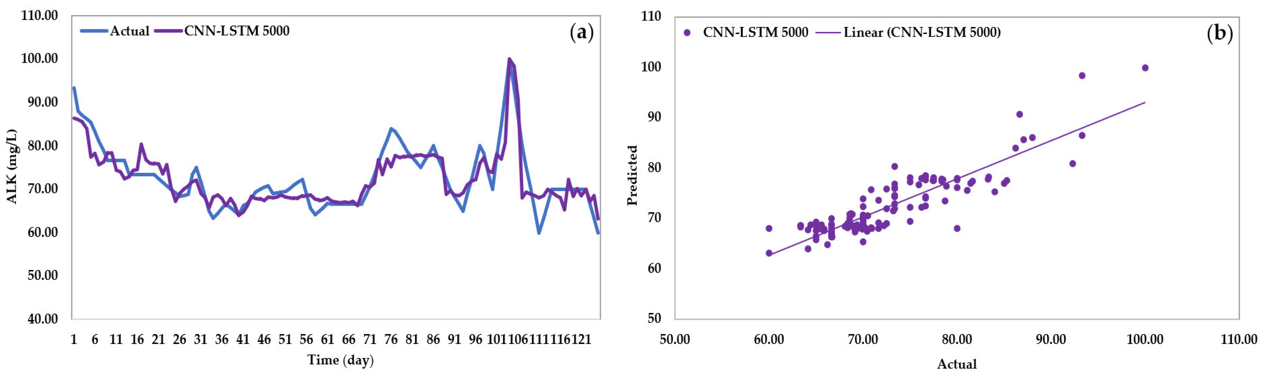
| CNN-LSTM 5000 epoch | 3.384 | 2.524 | 0.085 | 0.739 | 0.780 | 15 min 27 s |
Disclaimer/Publisher’s Note: The statements, opinions and data contained in all publications are solely those of the individual author(s) and contributor(s) and not of MDPI and/or the editor(s). MDPI and/or the editor(s) disclaim responsibility for any injury to people or property resulting from any ideas, methods, instructions or products referred to in the content. |
© 2024 by the authors. Licensee MDPI, Basel, Switzerland. This article is an open access article distributed under the terms and conditions of the Creative Commons Attribution (CC BY) license (https://creativecommons.org/licenses/by/4.0/).
Share and Cite
Jongjaraunsuk, R.; Taparhudee, W.; Suwannasing, P. Comparison of Water Quality Prediction for Red Tilapia Aquaculture in an Outdoor Recirculation System Using Deep Learning and a Hybrid Model. Water 2024, 16, 907. https://doi.org/10.3390/w16060907
Jongjaraunsuk R, Taparhudee W, Suwannasing P. Comparison of Water Quality Prediction for Red Tilapia Aquaculture in an Outdoor Recirculation System Using Deep Learning and a Hybrid Model. Water. 2024; 16(6):907. https://doi.org/10.3390/w16060907
Chicago/Turabian StyleJongjaraunsuk, Roongparit, Wara Taparhudee, and Pimlapat Suwannasing. 2024. "Comparison of Water Quality Prediction for Red Tilapia Aquaculture in an Outdoor Recirculation System Using Deep Learning and a Hybrid Model" Water 16, no. 6: 907. https://doi.org/10.3390/w16060907