
Bathymetric Modelling of High Mountain Tropical Lakes of Southern Ecuador

1
Laboratorio de Ecología Acuática (LEA), Facultad de Ciencias Químicas, Universidad de Cuenca, Av. 12 de abril S/N, Cuenca 010203, Ecuador
2
Departamento de Ingeniería Civil, Facultad de Ingeniería, Universidad de Cuenca, Av. 12 de abril S/N, Cuenca 010203, Ecuador
3
Departament de Biologia Evolutiva, Ecologia i Ciències Ambientals, Universitat de Barcelona, 08028 Barcelona, Spain
4
Subgerencia de Gestión Ambiental de la Empresa Pública Municipal de Telecomunicaciones, Agua Potable, Alcantarillado y Saneamiento (ETAPA EP), Cuenca 010101, Ecuador
5
Facultad de Ciencias Químicas, Universidad de Cuenca, Av. 12 de abril S/N, Cuenca 010203, Ecuador
*
Author to whom correspondence should be addressed.
Water 2024, 16(8), 1142; https://doi.org/10.3390/w16081142
Submission received: 21 February 2024
/
Revised: 31 March 2024
/
Accepted: 11 April 2024
/
Published: 18 April 2024
(This article belongs to the Special Issue Application of GIS Models and Remote Sensing in Water Quality Evaluation, Land and Coastal Zone Management)
Abstract
:Very little is known on high mountain tropical lakes of South America. Thus, the main motivation of this research was obtaining base bathymetric data of 119 tropical lakes of the Cajas National Park (CNP), Ecuador, that could be used in future geomorphological studies. Eleven interpolation methods were applied with the intention of selecting the best one for processing the scattered observations that were collected with a low-cost fishing echo-sounder. A split-sample (SS) test was used and repeated several times considering different proportions of available observations, selected randomly, for training of the interpolation methods and accuracy evaluation of the respective products. This accuracy was assessed through the use of empirical exceedance probability distributions of the mean absolute error (MAE). A single best interpolation method could not be identified. Instead, the study suggested six better-performing methods, including the complex methods Kriging (ordinary), minimum curvature (spline), multiquadric, and TIN with linear interpolation but also the much simpler methods natural neighbour and nearest neighbour. A sensitivity analysis (SA), considering several data error magnitudes, confirmed this. This advocated that sophisticated interpolation methods do not always produce the best products as geomorphological characteristics of the study site(s) together with observation data characteristics are likely to play important roles in their performance. As such, this type of assessment should be carried out in any terrestrial mapping of bathymetry that is based on the interpolation of scattered observations. Upon the analysis of the relative hypsometric curves of the 119 study lakes, they were classified into three average form categories: convex, concave, and mixed. The separated accuracy analysis of these three groups of lakes did not help in identifying a single best method. Finally, the interpolated bathymetries of 114 of the study lakes were incorporated into the best DEM of the study site by equalising their elevation reference systems. It is believed that the resulting enhanced DEM could be a very useful tool for a more appropriate management of these very beautiful but fragile high mountain tropical lakes.
1. Introduction
Worldwide, mountain regions provide important ecosystem goods and services, among which water resources are perhaps the most important for a significant lowland population that depend on highland runoff for irrigation, municipal and industrial water supply, hydropower production, and environmental services provided by river flows [1,2]. This runoff dependency of lowlands is projected to increase substantially by the mid-twenty-first century even under a mild (climate) change scenario [1]. But mountains are important not only because they contribute an important amount of runoff for lowlands; they also reduce the seasonal variability of flows in these lowlands [1]. Despite their importance for sustainable development, little is still known, particularly in tropical regions [3,4], about these very productive but, at the same time, very fragile systems, that are sensitive to rapid global development and climate change [2].
This is also the case for the lakes of these tropical systems, since they have received relatively little attention [3,5,6,7], despite the fact that, for water management, lakes, in general, and the ones with large volumes in particular, can be directly regarded as being important natural water storage spots and, as such, as being important water resources [8]. As an example, in Ecuador, the Cajas National Park (CNP) is a Ramsar site and key component of the “Macizo del Cajas” (MzC) Biosphere Reserve of the United Nations Educational, Scientific and Cultural Organization (UNESCO) that has more than 5955 lakes and ponds, among which, 322 are larger than 1 ha [3]. It is estimated that Cuenca, the third largest city of the country with circa 500,000 inhabitants, obtains about 60% of its drinking water from the highland tropical lakes of the nearby CNP. Nevertheless, this very important lake district, has been, traditionally, very little studied as a result of, among other reasons [3], the very difficult meteorological and topographic conditions that affect sampling/monitoring. It is not until the current decade that several limnological analyses have taken place in the CNP [3,4,6,9,10].
This, definitively, is in contrast with the importance of lakes for hydrological and biochemical cycles [4,11], that is, for sustainable development [8,9]. Therefore, their monitoring and surveying are fundamental not only for their appropriate management and conservation but also because lakes are also key indicators of watersheds at both local and regional scales [8,12] and can be used to learn about global and climate change effects and/or adaptation [8]. Therefore, the morphology of lake basins is a very important physical characteristic that influences physical, chemical, and biological parameters of lakes [12,13,14] and, therefore, their productivity. The morphology of a lake is the result of its origin and subsequent modifications caused, for instance, by water, wind, and sediment dynamics [12,13], which define whether lakes with similar surface areas are deep or shallow. In this regard, bathymetry is a key physical characteristic of lakes upon which geomorphological analyses are normally performed; its surveying or modelling is therefore important in the scope of lake management and research [13,14].
However, commonly, little information is given in scientific literature on the methodological approaches followed to model this important topographical characteristic, particularly in studies about tropical lakes [12,15,16,17]. One of the traditional ways of modelling lake bathymetry is by interpolation of observed point clouds surveyed through the use of a sensing instrument, such as a sonar [12,17], or even through the use of a remote sensing instrument [18,19]. Nevertheless, important differences in the representation of observed surfaces produced by different interpolation methods have been highlighted not only in the scope of topography or bathymetry [20,21,22,23,24,25] but also in the context of other types of civil engineering studies where thematic surfaces are generated on the basis of observed point clouds, such as meteorology [26,27,28], soil studies [28], hydrogeology [29,30], etc. Despite this, rarely, the use of interpolation methods for deriving thematic surfaces is preceded by a sound analysis of their suitability given the purpose of the study beforehand and/or the available data set, etc.
Therefore, the general objective of this research was obtaining base bathymetric data of tropical high mountain lakes of the CNP, Ecuador, by means of suitable interpolation methods; bathymetric data were obtained that could be used in future geomorphological studies that may in turn contribute to the conservation and better ecological management of these very fragile highland tropical lakes. The specific objectives were: (i) assessing the most accurate interpolation method(s) to build up the bathymetries of the study lakes given their morphological conditions and the main characteristics (i.e., accuracy, density, and distribution) of the available observations; (ii) inspecting their hypsometric properties to evaluate potential morphological differences among the study lakes; and (iii) incorporating the bathymetries of the study lakes into the most accurate digital elevation model (DEM) of the study site with the intention of developing an enhanced tool for management purposes. Hereafter, this manuscript presents the results of an extensive bathymetric surveying and modelling of high mountain tropical lakes of southern Ecuador, which, to the best of our knowledge, is one of the very few investigations of its kind applied on these little studied tropical lake ecosystems of South America.
2. Materials and Methods
2.1. The Study Lakes
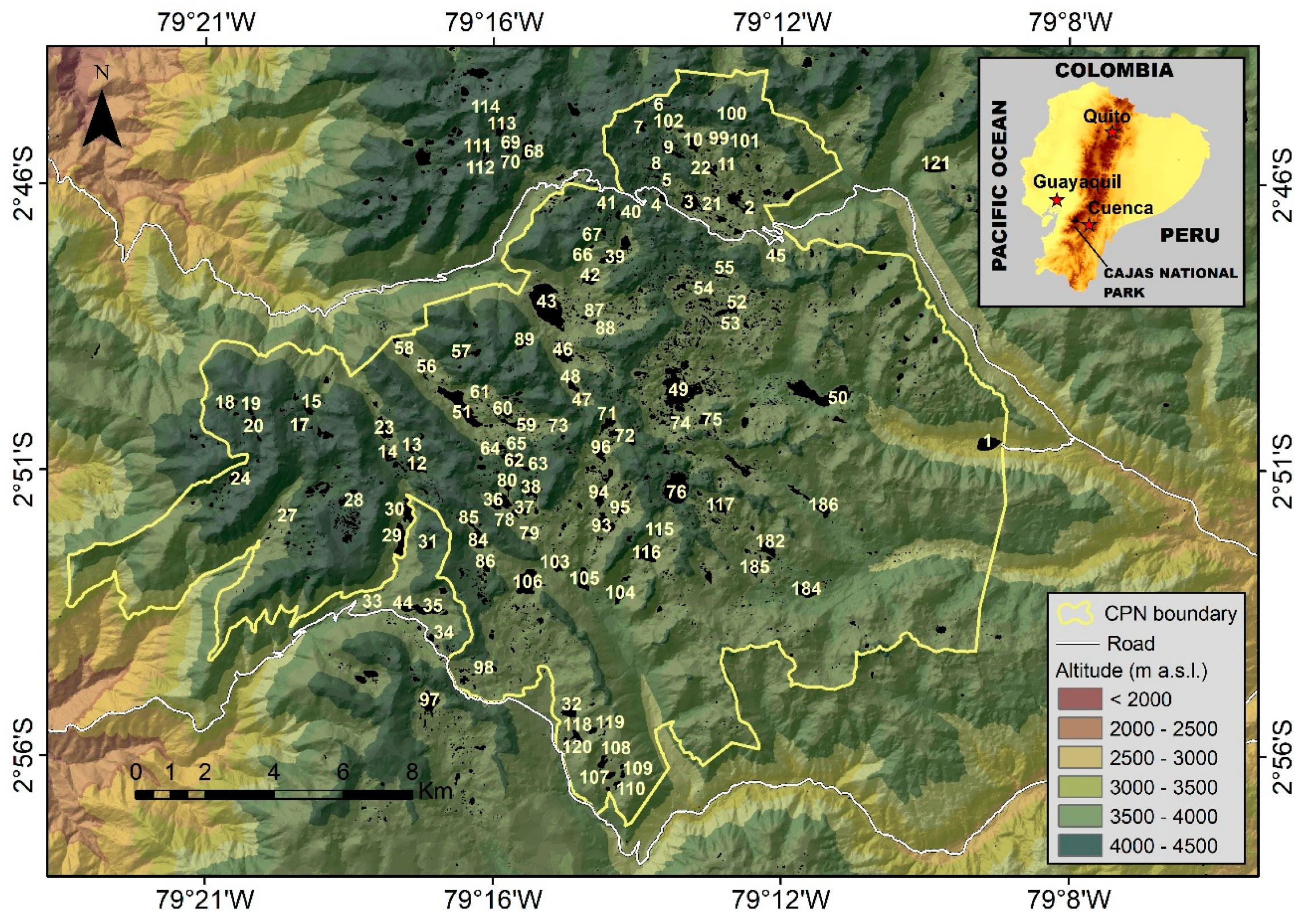
One hundred and nineteenth lakes were studied. Most of them (115) are situated in the Cajas National Park (CNP) in the south of Ecuador (Figure 1). Three lakes are situated to the south of the CNP, in the Quimsacocha volcano area, and one is in the Sangay National Park (SNP). The elevation of the CNP spans between 3150 and 4460 m above sea level (a.s.l.). The surface of the park is approximately 285 km2. Part of the CNP (about 34%) contributes to the Pacific Ocean, whilst the remaining area drains to the Atlantic Ocean system. The Pleistocene Tarqui volcanic bedrock is the main formation that includes rhyolite, andesite, tuff, pyroclastics, and ignimbrites [31]. The regional geomorphology and lakes were shaped by glacier activities until the late Pleistocene when the ice retreated around 17,000–15,000 years ago [32,33].
The main soil types at the region are non-allophanic Andosol and Histosols. Both types present dark-coloured epipedons characterised by high organic matter content, high porosity, low apparent density (400 kg m−3), and a high water retention capacity. Owing to these soil characteristics, most of the rainfall is retained in the soil and released gradually to the water courses, regulating the hydrology of these ecosystems [3]. The vegetation in 91% of the total extent of the CNP is herbaceous with a predominant presence of the genera Stipa and Calamagrostis [34]. With respect to the woody vegetation, Polylepis reticulata [35] is present above 3500 m a.s.l. and the high mountain forest (“bosque montano”) is present between 2900 and 3400 m a.s.l. The main impacts of land use and human activities on vegetation are due to tourism, fishery, grazing, and localised burning of the vegetation.
Only one lake is situated below 3500 m a.s.l.; two of them are located above 4300 m a.s.l. Most of them have maximum depths deeper than 4 m. Their surfaces, except that of one of them, are greater than 0.005 km2; four of them cover surfaces greater than 0.46 km2. Their storage volume also varies in a wide range [3].
2.2. Digital Elevation Model (DEM) of the Study Site
Since the year 2015, there have been some acceptable elevation data about the study area in the form of a DEM provided by the Ecuadorian government’s project SIGTIERRAS (www.sigtierras.gob.ec; accessed on 15 May 2023). It is the product of processing light detection and ranging (LiDAR) point clouds that were achieved for most of the continental territory of Ecuador. The spatial resolution of the DEM, which is in raster format, is 3 × 3 m2 for the Sierra region, 4 × 4 m2 for the Costa region, and 5 × 5 m2 for the Amazonian region. Its vertical accuracy is ±1.5 m for the Sierra and Costa regions and ±3.0 m for the Amazonian region.
The DEM of the study area was available as a series of segmented pieces or tiles (Figure 2a) having a size of 770 rows and 775 columns and a resolution of 3 × 3 m2. Although the DEM tiles were available directly in the same system of coordinates used in this study (i.e., UTM 17-S, WGS84), the orientation of the original segmentation axes differed slightly from the respective orthogonal orientation of the current axes, which produced few pixels of the borders having a no-data attribute. Thus, a nearest neighbour (NN) resampling (interpolation) approach [20,36] was applied to estimate their topographical attributes. Only the attribute values of the few no-data pixels were modified; the values of the other pixels remained unaltered.
All of the DEM tiles were mosaicked (Figure 2b) so that the domain of the resulting terrain model covered the extent of the CNP and all the study lakes, including lake 90 (“Laguna Chullacocha”) located far to the south of the CNP boundary (Figure 2b) in the Quimsacocha volcano area.
The congruency of the mosaicking operation was always tested by comparing the resulting mosaic product and several of the original DEM tiles. Mosaicking took place in TERRSET version 18.0 using two approaches; namely, through the use of (i) the MOSAIC command and (ii) the CONCAT command. Unfortunately, both approaches incorporated artificial changes to the topographical attribute values of many of the pixels of the original DEM tiles. Some of these changes were important. The mosaicking approach available in ARCGIS version 10.0 was very successful and no artificial changes of the original terrain attribute values happened. Therefore, the product of this mosaicking process was adopted for the rest of the study. The mosaicking operations in either TERRSET or ARCGIS, including the cross-checking of the quality of the final product, were carried out in batch mode, using appropriate TERRSET macro language (IML) and ARCGIS Python subroutines.
Finally, the mosaic product was trimmed to obtain the biggest and most complete DEM (rectangular) domain, covering all of the spatial features of interest of this study (i.e., the CNP’s extent and the study lakes’ locations) and without no-data pixels in some parts of its borders. Figure 2 depicts the rectangular polygon that defines the DEM domain that was used in this study.
This product is the best DEM of the CNP and surroundings. Nevertheless, it does not include accurate bathymetric data of the study lakes (in many cases, it includes flat or nearly flat bathymetric surfaces in the spots of the 119 study lakes), which is an aspect that does not support the appropriate management of these lakes. Therefore, this study aimed at incorporating the generated bathymetric models of these lakes into the abovementioned DEM of the study site.
Further, this DEM was not available at the moment that the bathymetric field surveying took place nor when the bathymetries of the study lakes were modelled using these field observations. Therefore, the DEM data of the surroundings of the study lakes were not available during the initial modelling of the bathymetry of the study lakes.
2.3. Bathymetric Surveying
In the surveying planning stage, the average perimeter (i.e., littoral) of every one of the surveyed lakes was digitised from aerial photos, which were orthorectified and georeferenced and have a 30 × 30 cm2 resolution (www.sigtierras.gob.ec, year: 2011, zone: CNP). The digitisation process was performed by using ARCGIS. The scale of cartographic digitalisation was 1:5000. These lake perimeters were used in this study as zero depth data (Figure 3), as well as for planning on the number of surveying transects and the spacing between them, which depended on the size of the lake being surveyed. Both the number of transects and their spacing were fixed aiming at achieving the best possible data resolution and density, even in the case of the larger study lakes. This is because prior experiences suggested that data proximity is rather important when applying interpolation methods to data clouds. Thus, for lakes with surface areas larger than 0.2 km2 the transect spacing was around 100 m; for lakes with areas between 0.1 and 0.2 km2, the spacing was around 50 m; and for lakes with areas smaller than 0.1 km2 the spacing was about 25 m. Normally, the direction of the transects runs parallel to the main longitudinal and transversal axes of the surveyed lakes, forming a grid (Figure 3). In any case, the distance between the bathymetry points did not exceed 5 m. In the shallow lakes and ponds, near their littorals where the use of a boat was not possible, measurements were taken at several points of the water body using a topographic measuring rod.
The bathymetric survey (Figure 3) was carried out in the period beginning-2014–mid-2015 with the aid of (i) an inflatable rubber boat (Navigator II, RTS, Hong Kong, China), approximately 3.5 m long, which was equipped with a propeller (2 HP, Yamaha, Japan) and (ii) an multi-echo sounder Humminbird model 1198c SI (Eufaula, AL, USA) [37] that recorded the depth to the bottom of a given surveyed lake. The echo-sounder can measure using the frequencies 83 kHz, 200 kHz, 455 kHz, or 800 kHz, depending on the chosen surveying program, in combination with either beam angles of 20°, 60°, or 86° [37]. This is a fishing echo-sounder system; it is not a specialised bathymetric instrument. Its choice depended particularly on its price as abundant financial support was never available for this study. However, indirectly, the use of a non-specialised instrument, that is relatively low-cost, was an appealing challenge that may reflect the management conditions in other high mountain locations of Ecuador and/or the South American region. Owing to the remoteness of the study area and the extreme high mountain (above 3500 m a.s.l.) weather conditions, the field work was extremely physically demanding since transportation of the equipment had to be performed mainly on foot, sometimes with the help of horses, enduring these difficult conditions for several days a week.
Because a fishing echo-sounder system was used in this study for acquiring bathymetric observations, which is not a generalised approach, and definitively less generalised by the time that the original surveying took place, and because most of the worldwide application of these systems do not report any error accuracy information, an assessment of the associated random measurement errors was carried out. Nevertheless, neither a very accurate testing set of bathymetric observations for accurately assessing on these random measurement errors and “calibrating” our instrument nor (usually very expensive) specialised instrument(s) to acquire the testing data was available. Therefore, an approximated approach to estimate these errors was implemented in five of the study lakes, namely, Llaviuco (ID = 1 in Figure 1), Toreadora (ID = 3), Larga (ID = 39), Luspa (ID = 43), and Sunincocha Grande (ID = 51). In these lakes, the engine of the boat was stopped in some spots that were selected (while sitting on the boat), using the subjective knowledge of the sonar and boat operators on the potential shape characteristics of every one of those study lakes.
Windy conditions, and consequent wave action, are frequently prevailing in the study site. Despite this issue, it was assumed that the boat remained still, “for a while”, in exactly the same spot. Some readings, from 5 to 10 (subjectively, depending on wind conditions), were then carried out. The original planning expected to collect more readings in every “fixed” location but wave action and consequent boat displacement did not enable this. This approach was applied under the assumption that for, ideally, “many” sonar readings, collected at exactly the same spot, the average value would be the “most probable” depth in that spot and the respective standard deviation would be an estimate of the random measurement error magnitude (i.e., errors can be positive or negative) in that spot.
There are some practical aspects that would affect some of the assumptions of this approach. One of them is the relatively low number of sonar readings for every visited spot that would affect the “accuracy” of the estimates of probable depth and associated random measurement error. Additional aspects are the boat shifting owing to wave action and the GPS accuracy, ranging from 1 to 5 m upon satellite availability that depends (in turn) on cloudiness. Both aspects would affect the assumption of surveying in exactly the same location; the first one because of a real boat displacement, whilst the second one because of an apparent (i.e., false) boat displacement. Despite them, it is believed that this simple approach is very appropriate in applied research projects like the current one for having at least a rough idea of the random measurement errors, particularly when there is a lack of additional, more accurate, data (or instrumentation to acquire them) for a more accurate estimation of these errors. These estimated errors were assumed overall for all the study lakes.
Given the abovementioned sources of uncertainty that can affect the sonar readings, the protocol for capturing the bathymetric data aimed at reducing them as much as feasible. Hereafter, the field surveying with the Humminbird® multi-echo sounder capable of emitting 5 pulses s−1 [37] was conducted assuming that, at a low beam angle (20°) and a frequency of 200 kHz (Dual Beam PLUS™ and High Definition Side Imaging®), the accuracy of the depth observations would be the best, with acceptable range and resolution, which is suitable for surveying relatively shallow depths. Higher errors were expected to occur for a beam angle of 60° and a frequency of 83 kHz, used particularly for deeper depths. Nevertheless, using higher frequencies (High Definition Side Imaging®) and wider beam angles, in relatively shallow depths, the accuracy was also expected to be acceptable.
Further, we placed the transducer on the side of the boat to avoid any turbulence from the boat propeller (located in the rear of the boat). With the same intention, the front of the boat was stabilised as much as feasible by the weight (ballast) of one of the operators sitting there; in this way, we hoped to minimise the effect of wave action on the pitch and roll of the boat (and transducer), and, as such, to reduce the possibility of adding more error to the measurements. Further, the two boat-and-instrument operators hardly moved while surveying at an average (constant) boat speed of about 3 m s−1.
2.4. Bathymetric Modelling
2.4.1. Splitting the Observations into Training and Evaluation Data Sets (Split-Sample Test)
The bathymetric modelling of the study lakes took place in the year 2015 after the surveying campaigns were over. The process to produce the digital bathymetric description of the surveyed lakes and the derived geomorphological products included (Figure 3): (i) writing all of the necessary subroutines for processing the information, carrying out the interpolation calculations, and analysing the quality of the interpolated products; (ii) processing the data achieved in the field so that any incongruence (duplicates, outliers, etc.) could be filtered out and implementing a protocol to avoid errors in the processing and storage of the observed data; (iii) saving the information with the right digital format for the forthcoming steps; (iv) applying the developed subroutines for the bathymetric interpolation of the sonar observations of every one of the 119 study lakes and immediate application of a low-pass Gaussian filter for smoothing the interpolation product and eliminating potential pitholes artificially generated by the interpolation methods; and (v) assessing the quality of the corresponding bathymetric products of the study lakes as a function of the tried interpolation methods. The task-specific subroutines developed for most of these processes were programmed with the high level programming language VISUAL BASIC (VB) for running within the automation environment Scripter of SURFER version 16 in combination with the Practical Extracting and Reporting Language (PERL) high level programming language and, to some extent, the MATLAB version R2019a programming environment.
The second step included the integration of the elevation (depth) data collected in the field with the data derived from the digitalisation of the orthophotos (i.e., perimeters of the lakes associated with zero depth) so that the feasible bounds of the posterior interpolation process could be defined properly. For filtering out some potential pitfalls of the data collected on the field, these lake perimeters, as well as other relevant spatial information and field annotations, were used. This filtering was implemented with the aid of the geographical information system (GIS) software ARCGIS. For the third step, some of the task-specific subroutines were used, ensuring compatibility with SURFER that was later applied for the interpolation process.
The fourth step involved using SURFER for obtaining the digital bathymetric surfaces of the surveyed lakes, considering the set of observations Zci (Figure 3). SURFER was also used to apply the low-pass Gaussian filter on the interpolated bathymetric surfaces immediately before the evaluation of the performance of the interpolation methods. Only a single pass of the filter was applied. Because the same type of bathymetric observation was used for the interpolation process and later for the evaluation of the interpolated bathymetric models, it is believed that this simple smoothing process does not bias the assessment of the performance of the interpolation methods. The fifth step consisted in finding the best interpolation algorithm for the current bathymetric data on the basis of judging the elevation (i.e., depth) accuracy of the resulting interpolation product by means of the split-sample (SS) test. Similarly to what is normally carried out in dryland topographic analyses [20], the accuracy of the interpolation products was based (Figure 3) mainly on the comparison of the elevation characteristics of a set of (field) observations (Zei), selected randomly and not used in the interpolation process, and the respective depths of the interpolation product (that is, through the consideration of model residuals).
In this study, 20% (i.e., Mi/Ji; see Figure 3) of available sonar observations were preferred for this purpose; nevertheless, the congruency of the results of the analysis was cross-checked by considering other data proportions, such as Mi/Ji = 30% and Mi/Ji = 40%. A further congruency analysis consisted in repeating the selection of the elements (i.e., sonar observations) of Zei (and Zci) and the respective quality assessment approach a couple of times. This was implemented because, owing to the random selection of the testing observations for building up Zei, for the same Mi/Ji value, different sonar observations conform to two given realisations of Zei. The results reported herein correspond to one of these realisations; in general, the congruency tests emphasised them. Data handling, including the random splitting of available observations into training (Zci) and evaluation (Zei) data sets (i.e., SS test), and the statistical assessment of the performance of the interpolation algorithms (Figure 3) were performed with task-specific subroutines programmed with PERL.
2.4.2. Interpolation Methods
In total, eleven interpolation methods (i.e., K = 11, in Figure 3) were applied on the sonar observations of the 119 study lakes, which implied preparing task-specific VB subroutines for SURFER that produced a total of 1309 bathymetric surfaces. The quality assessment of all of these bathymetric surfaces was also carried out with SURFER using task-specific VB subroutines prepared with this purpose in mind. In the forthcoming text, a target node refers to the point for which an interpolated attribute is defined based on the values of neighbouring observations (situated on grid nodes). The tested interpolation methods were the following ones [12,15,16,20,21,22,24,25,26,27,30,36,38,39,40,41,42,43,44,45]; we decided that for the objectives of this study, there was no need for testing additional interpolation methods.
The inverse distance to a power (IDW) method [15,20,22,23,24,25,26,27,28,30,39,40,43,44,45] is a weighted average interpolator, within which the influence of an observation, relative to the target node, declines with distance as a function of the considered power: the greater the weighting power, the lower the effect of farther observations on the target node. A power value of 1 was considered herein. Further, a non-zero smoothing parameter was defined. IDW uses this parameter to reduce the “bull’s-eye” appearance of the generated contours, preventing, as much as feasible, any observation close to the target node having an overwhelming (interpolation) weight. This was performed despite the fact that a thorough pre-processing approach was applied to remove potential data anomalies before applying the study interpolation methods, minimising in this way the potential presence of a “bull’s-eye” appearance. A very similar method is modified Shepard [41,42], which uses local least squares for reducing the bull’s-eye effect (when related data anomalies are present among the observations).
The natural neighbour method [22,24,27,38,44,45] considers a set of Thiessen polygons that are formed with the observations, except the target node. When it is added into the domain of polygons some of the neighbouring polygons shrink in size to accommodate the respective target node’s Thiessen polygon. The proportions of their original areas that are “borrowed” to form the newer Thiessen polygon are used as weights in a weighted average of the neighbouring observations to define the interpolated value of the target node. On the other hand, the nearest neighbour method [20,25,26,30,36,39] assigns the value of the nearest point to each target node.
The moving average method [36,38,39] assigns values to grid nodes by averaging a minimum number of neighbouring observations within the target node’s search window.
Polynomial regression [28,36,38,39,43], although not strictly an interpolator, is used to define large-scale trends and patterns in the observations with which the “predicted” surface is built. The local polynomial method [38,39,43] assigns values to target and grid nodes by using a weighted least squares fit. However, instead of fitting the polynomial to the entire data set of observations, as in the case of polynomial regression, it is fitted to a local data subset defined by a window, that in the case of SURFER is a search ellipse.
The triangular interpolation network (TIN) [16,20,21,22,23,24,28,39,40] uses the optimal Delaunay triangulation, so that no triangle edges are intersected by other triangles. Each triangle, formed by three observations, defines a plane where the potential target node is lying. Commonly, as in the current case, the TIN method is used combined with linear interpolation along the edges of the triangles. The TIN method works best when observations are evenly distributed over the interpolation domain (grid area); otherwise, the TIN results in distinct triangular patterns on the interpolated surface.
Kriging is a geostatistical gridding method that attempts capturing the essential observation’s trends while dealing with anisotropy [12,16,22,23,24,25,26,27,28,36,39,43,45,46,47]. It is known to be good for avoiding bull’s-eye type interpolation products. Ordinary Kriging was applied herein since it can still produce accurate interpolated surfaces from observations [38], despite assuming that the variation in elevation values is free of any structural component (i.e., drift). Further, Kriging can be customised to a particular set of observations by specifying an appropriate variogram model [43,46]. Since it is very flexible and it has been proven useful in many applications, it has become very popular; nevertheless, its application does not always involve a (prior) suitability analysis.
The minimum curvature method [39,40,44,48] generates a smooth, thin, and linearly elastic interpolated surface (spline), having continuous second derivatives and minimal total squared curvature, that passes as closely as possible through each of the observations.
Radial basis functions [24,27,38,43,47] are data interpolation methods (kernel “functions”) that aim at producing a smooth surface and that are analogous to variograms in the Kriging method. The multiquadric method was chosen for the current analysis; other available functions in SURFER are: inverse multiquadric, multilog, natural cubic spline, and thin plate spline ([22,24,25]). Default values were chosen for other parameters such as the shape factor.
Similarly, data metrics [38] is a collection of methods that, however, produce grids of information about the observations but, in general, not weighted average interpolations. Therefore, this SURFER gridding method was not inspected in the context of this research.
2.4.3. Assessing the Accuracy of Interpolation Methods
Model performance indexes are normally used to characterise the quality of the empirical interpolation algorithms used for representing the shape of the terrain [20]. These are generally based on residuals (resq [L]) and the difference between the q-th bathymetric observation (Ztq [L]) and the respective model prediction (Zpq [L]). Depending on the form of the model performance index, they can measure [49] either: (i) the average (model) systematic error; (ii) the average combined systematic and random error; or (iii) the correlation among Ztq and Zpq.
Hereafter, the mean absolute error (MAE) [L] defined as the average of the absolute value of residuals (|resq| [L]) was particularly used in this study as a measure of the average (systematic) error of every one of the bathymetric models. Using the absolute value of residuals avoids residuals of the opposite sign cancelling each other out and producing a false depiction of accuracy of the modelled bathymetric surface [20]. Its optimal value is zero and has also been used in past lake bathymetric assessments including satellite-based bathymetric (SDB) studies [50,51] as well as in other civil engineering interpolation studies [23,26]. This was carried out for every one of the (11) tried interpolation methods and for both the training and evaluation data sets (in the scope of a traditional split-sample (SS) test). For carrying out the assessment automatically, this involved developing appropriate subroutines in TERRSET, ARCGIS, and R, as well as programming task-specific subroutines with PERL. In general, GNUPLOT version 5.4 was used for plotting purposes.
For a given interpolation method, the respective 119 MAE values were further processed so that an empirical exceedance probability distribution was generated for the method on the basis of the following plotting position of a quantile formula:
where Pm is the empirical exceedance probability for the position m within the data set, and α and β are the constants of the plotting position estimator. When α = 0 and β = 0, Equation (1) is the Weibull formula, which is considered to be an unbiased (empirical) exceedance probability for some distributions [52]. As such, it was preferred in this study, although alternative plotting position methods were also explored, such as Blom (α = 0.375 = β) and Gringorten (α = 0.44 = β). The quality of the bathymetric products was assessed by accounting for the differences in terms of the shape and evolution of the empirical probability distribution curves of the eleven interpolation methods: the curves that are made of lower residuals correspond to more accurate interpolation methods (given the morphological properties of the study lakes and the bathymetric data characteristics). PERL subroutines were used to carry out the plotting position analysis; further, GNUPLOT subroutines were prepared to visually examine the results of this analysis.
Once the best interpolation methods were identified through the above statistical and graphical approaches, the respective modelled bathymetric surfaces were used in the scope of the further analyses of this research.
2.4.4. Sensitivity Analysis of the Effect of the Magnitude of Random Measurement Errors on the Accuracy of the Interpolation Methods
Given that a simple approach was implemented to estimate the random measurement errors associated with the use of the sonar fishing system to collect bathymetric observations, it was decided to carry out a sensitivity analysis (SA) on the effect of the magnitude of random measurement errors on the accuracy of the products of the study interpolation methods. This was carried out with the intention of cross-checking the congruency of the evaluation of the best interpolation method(s) as a function of the random measurement errors.
Thus, random errors were added to the original bathymetric observations, considering three depth classes, namely, (i) 0.001 m to 25 m; (ii) 25 m to 50 m; and (iii) more than 50 m. The higher error magnitudes were applied on the class of deeper depths, whilst lower error magnitudes were applied on the class of shallower depths. Positive and negative errors were added to the original observations. Several error scenarios were run. In terms of the magnitude of the errors, minimum values considered in the analysis are in the order of 15 cm, whilst maximum error values in the order of 5 m were also considered.
2.5. Inspecting the Hypsometric Properties of the Study Lakes
The average form characteristics of the study lakes were evaluated through the use of hypsometric curves of all the 119 surveyed study lakes. This was performed for every one of the six interpolation methods that produced the best bathymetric products. Given the significant variability of maximum depths of the study lakes, from a few metres to several tens of metres, the hypsometric curves were constructed relative to the maximum depth of every study lake [53,54]. In this way, the vertical range of variation of every lake’s hypsometric curve is expressed as a percentage (or as a fraction) from 0% to 100% rather than in absolute length units. Further, for every study lake, the horizontal area associated to every vertical depth of the lake’s relative hypsometric curve was also expressed in relative terms with regard to the total surface area of the lake. As such, the respective range of variation also spanned from 0% to 100%. This enabled the comparison of forms of lakes of different sizes (surface area) and depths, so that potential morphological similarities (or dissimilarities) among the study lakes could be evaluated.
It must be observed that on the contrary to what is normally performed in hydrological applications that construct the hypsographic curve of a drainage basin using the horizontally projected area of the drainage basin above the elevation contour line of interest [54], in this research, the horizontal area of the lake’s basin at the depth (or elevation) of interest was considered [13,14]. That is, maximum area happens at the surface, whilst the zero area is reached at the maximum lake’s depth.
Hereafter, plotting the depth in reverse order, the 45° diagonal line that connects the 100% level of both the depth and area axes is the reference line for judging the average lake’s shape. This average form can be [13,14]: “convex” (i.e., when the relative hypsometric (RH) curve is systematically above the reference line), “concave” (i.e., when the RH curve is systematically below the reference line), or “mixed” (i.e., when the RH curve has portions of it above and below the reference line). Prior to this analysis for determining the average form of the study lakes, the sensitivity of the form of RH curves to vertical resolution was investigated.
Because interpolation methods with a similar accuracy could generate quite different spatial patterns [20,28], the accuracy of the better-performing interpolation methods, modelling the different spatial patterns that characterise the three lake forms used in this study, was also investigated by constructing the exceedance probability distributions of the three average lake forms for every one of the better-performing interpolation methods. This is a complementary accuracy assessment that was implemented to support the process for elucidating the best interpolation method for this study.
Visual basic subroutines were prepared to calculate with SURFER the hypsometric curves of all the 119 study lakes and best interpolation methods, as well as different vertical resolutions. PERL subroutines were prepared to post-process the SURFER results and automatically calculate the RH curves of the study lakes, as well as for calculating the empirical exceedance probability distributions of the interpolation methods. A MATLAB subroutine was prepared to determine the average form of every one of the study lakes. GNUPLOT subroutines were set to visually examine the results of this analysis.
2.6. Incorporating the Lake Bathymetry into the Digital Elevation Model (DEM) of the Study Site
This part of the analysis was also carried out in the preparation of complementary research dealing with the remote sensed modelling of the bathymetry of the study lakes using Landsat imagery products. Five of the one hundred and nineteen lakes were not considered in this part of the study because their surface area was rather small and, as such, could not be well described, with an acceptable number of pixels, by the rather coarse satellite imagery resolution (i.e., 35 m). Thus, 114 lakes were considered in this part of the study.
Owing to the lack of a precise and easy-to-transport topographical instrument, the bathymetry surveying of the study lakes could not be connected accurately to the surrounded topography. This connectivity was based entirely on a GIS process, which consisted in recovering from the DEM the respective elevation of the lake’s polygon (perimeter or littoral) that was used in this study as the zero-depth reference when modelling the lake’s bathymetry. A simple line-to-raster operation was applied to define a “perimeter” mask with the aid of which the elevation data from the DEM could be extracted only for the perimeter of the lake. The average elevation of this lake’s perimeter topography was then used as the elevation of the reference polygon (lake’s perimeter). For all the study lakes, the standard deviation associated to this mean perimeter elevation was relatively low, in the order of a few tens of centimetres, which stressed the confidence in the mean elevation value as being representative of the elevation of the lake’s perimeter.
Therefore, once the elevation of the reference polygon was known, the elevations of the other internal pixels of the lake’s bathymetry were also known, then the lake’s bathymetry was finally incorporated into the DEM of the study site. This process was automatically implemented for all the 114 study lakes with both TERRSET and ARCGIS GIS software to cross-check the congruency of the respective enhanced DEM product. The latter was the main congruency approach applied to all of the study lakes: the two products of the GIS software were identical.
Further, as already stated, no accurate-enough DEM data of the surroundings of the study lakes were available during the initial modelling of the study lakes. Thus, a second bathymetric modelling process took place more recently, this time considering (i) the field survey information; (ii) the zero-depth digitised perimeters of the study lakes; and, additionally, (iii) some DEM data of the surroundings of the study lakes. This newer modelling was carried out to explore on whether this newer DEM-based data set could significantly affect the interpolated bathymetry nearby the shore of the study lakes. For determining the DEM-based data that were used in this second modelling exercise, a 45 m wide buffer around the perimeter of every study lake was defined from where DEM data were sampled randomly, as was carried out within the lake perimeter. This newer data set was further processed to be expressed as “negative depths” in the context of the above-depicted interpolation process. For every study lake, the external bound of the buffer was used this time as the interpolation bound (whilst in the initial modelling exercise, this bound was the lake’s perimeter). Comparison of the bathymetric products of the first modelling exercise with the ones of the second exercise was implemented within the perimeters of the study lakes (common extent) and was carried out through simple raster map algebra, using all of the pixels within the lake’s perimeters. It was carried out with TERRSET and revealed in most of the cases almost imperceptible changes with respect to the original bathymetries, as expected, nearby the shores of the lakes. This encouraged using the original bathymetric products throughout the rest of the study.
3. Results
3.1. Bathymetric Surveying
Figure 4a shows the estimated random measurement errors obtained in 5 of the 119 study lakes, as a function of the (water) depth. Maximum random errors in the order of ±47 cm were estimated, paradoxically, not for the deeper depths but for the mid-range depths and shallower ones. For deeper depths the maximum random errors were in the order of ±33 cm. The minimum random error was of about ±15.5 cm recorded for the deeper depths. These results point to a very acceptable (overall) accuracy of the surveying sonar instrument (and approach), given that it is not a specialised instrument and that there are several different sources of data uncertainty (small and light boat, wave action, relatively low GPS accuracy, etc.) besides the quality of the sonar instrument itself that is designed and used worldwide for recreational boat navigation.
Further, Figure 4b shows the transects that were used for the surveying of one of the deepest study lakes, Luspa (surface area: 0.77 km2). The figure depicts that the field work resulted in detailed data collection networks for the study lakes, even in the case of the larger ones. This is in line with the aim of the study of collecting the highest possible amount of observations to ensure sufficient data proximity (i.e., acceptable data density).
The figure also illustrates the distribution of training (80%) and evaluation (20%) bathymetric observations that were randomly selected and used in the scope of the SS test. The figure suggests a kind of uneven spatial distribution of the observations used in the evaluation stage of the bathymetric modelling, with more observations concentrated in certain areas of the study lake than in others. This is believed to be the consequence of preserving, in the context of the random selection of the SS data sets, the order in which the observation points were acquired throughout the surveying process; otherwise the spatial distribution would be more even. It was decided to keep the data collection order in the random process to preserve some surveying decisions that were adopted in the field, given the importance of certain morphological features present in the study lakes and that were noticed once the operators were in situ. Nevertheless, it is believed that this aspect does not affect the results of this study as all the interpolation methods were exposed to exactly the same data sets in the SS test and the evaluation data distribution reaches practically the full extent of the different surveying networks of transects of the 119 study lakes.
Finally, Figure 4c depicts the resulting bathymetric model for the Luspa lake when using one of the six best-performing methods (natural neighbour). The figure shows the sharp interpolated surface that was obtained for this large lake, given the significant amount of sonar observations available for the respective bathymetric modelling, as well as the application of the low-pass Gaussian filter on the interpolation product.
3.2. Bathymetric Modelling
When using 80% of the observations for training (and 20% for evaluation) the running times for both processes (considering all the study lakes and interpolation methods) were 18 min and 8.5 min, respectively (with a very narrow standard deviation, in the order of 5 s). When using 70% of the observations for training and 30% for evaluation, the running times were 16 min and 8.0 min, respectively, also with a very narrow standard deviation, in the same order. This information was recorded on a PC running Windows 7, having a RAM of 4 GB and equipped with an Intel(R) Core(TM) i7-4770 processor. The processes were not run recently, using modern PCs; so, it is not possible to provide comparable information when using modern hardware.
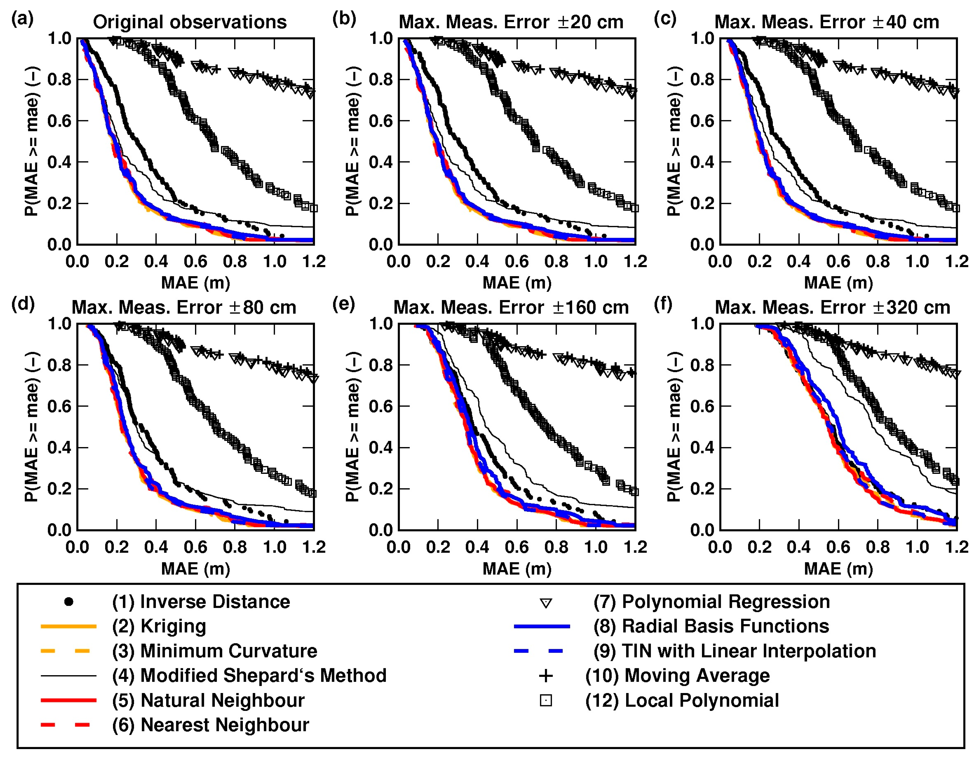
Figure 5 shows the empirical exceedance probability distributions of the mean absolute error (MAE) of residuals, as a function of the tried interpolation methods, for the evaluation phase of the split-sample (SS) test. Every one of the eleven probability distributions included in every plot of the figure corresponds to one of the eleven study interpolation methods and is made of 119 points (one per study lake). The calculation of the probability distributions of MAE implied a significant amount of computations per study lake and per interpolation method.
Although Figure 5 corresponds to the evaluation phase of the SS test, the respective results are very similar to the ones obtained for the training phase. The shape of the empirical exceedance probability distributions was nearly the same, independently of the plotting position formula that was used (Figure 5a–c). Thus, for the purpose of assessing the accuracy of the bathymetric products of the interpolation methods, either plotting position formulation may be suitable. The Weibull plotting position formula was further used in this study.
Furthermore, the shape of the distributions varied only marginally as a function of the size (density) of the evaluation data set (i.e., the amount of bathymetric observations kept for evaluation in the framework of the SS test) as depicted by Figure 5a,d,e that illustrate the resulting empirical probability distributions for different sizes of the evaluation data set, say, 20% of total available observations, 30%, and 40%, respectively. It is worth noticing that, since the sonar observations of lake bathymetry were selected randomly, even if the size of the evaluation data set (and, consequently, of the training data set) was the same for different runs of the latter assessment, every run used a different set of bathymetric observations (randomly chosen). Despite this, the results depicted in Figure 5a,d,e may be considered as representative of this latter assessment on the effects of the size of the evaluation data set.
The figure also reveals that there is a group of interpolation methods that perform better than the rest, as their empirical exceedance probability curves are very similar. These are Kriging (ordinary), minimum curvature, natural neighbour, nearest neighbour, multiquadric (a radial basis function), and TIN with linear interpolation. Their respective curves are drawn in colour in Figure 5. It should be observed that the accuracies of the IDW method and of the modified Shepard’s method, a special case of the IDW [48,55], are not that much inferior. Notwithstanding, the remaining methods steadily produced bathymetric products of clearly inferior quality; particularly, the methods polynomial regression and moving average.
These results were systematically observed for either size of the training (and evaluation) data set (Figure 5a,d,e). Because their MAE probability distributions overlap, any of the six better-performing interpolation methods could be used for modelling the bathymetry of the study lakes, given the morphological properties of the study lakes and characteristics of the bathymetric observations.
Figure 6 depicts the results of the sensitivity analysis (SA) of the effects of random measurement errors on the performance of the interpolation methods modelling the bathymetry of the study lakes. For every study lake, 80% of the observations were randomly selected for model training and the remaining 20% for model evaluation; once these two data sets were defined, they were kept constant throughout the analysis. Every plot in the figure corresponds to one of the tested error scenarios, which is described in the title of the plot by means of the maximum error magnitude considered in the scenario.
The figure indicates that, congruently, the MAE values increased as the magnitude of the random error measurement increased, which meant that, in the higher error scenarios, the empirical exceedance probability curves shifted toward higher MAE values. The figure also reveals that, even for maximum error magnitudes reaching 3.2 m (for the class of deeper depths; Figure 6f), the conclusions on the performance of the interpolation methods remained unaltered, as the distribution of the empirical exceedance probability curves remained practically unchanged for every scenario. Although not shown in this figure, other scenarios of higher error magnitudes confirmed the same tendency of the MAE exceedance probability curves, confirming the same six better-performing interpolation methods.
3.3. Inspecting the Hypsometric Properties of the Study Lakes
The analysis revealed that the shape of the RH curves is influenced by the vertical resolution used to derive them. The shapes of the respective RH curves are, in general, similar for resolutions 0.10 m (Figure 7a) and 0.25 m (Figure 7b). However, Figure 7c depicts that, for a resolution of 0.50 m, the shapes of the RH curves of some lakes are significantly different from the respective shapes that are obtained for the finer vertical resolutions. Particularly, the shapes of the RH curves of shallow lakes are affected by coarser vertical resolutions (Figure 7c); the finer the vertical resolution, the smoother the RH curves are (Figure 7a) and the larger the computational effort to derive them.
On the other hand, Figure 8 illustrates the general classification of the form of the study lakes determined by the position of their RH curves with regard to the reference line. The RH curves were determined considering a 0.10 m vertical resolution and the products of the Kriging (ordinary) method. The analysis showed that most of the study lakes (i.e., 70% of them) could be regarded as having a convex form, only 5% of them have a concave shape, whilst 25% of them have mixed form properties. Although not shown, the same analysis applied on the products of the other better-performing interpolation methods revealed similar results about the form classification of the study lakes.
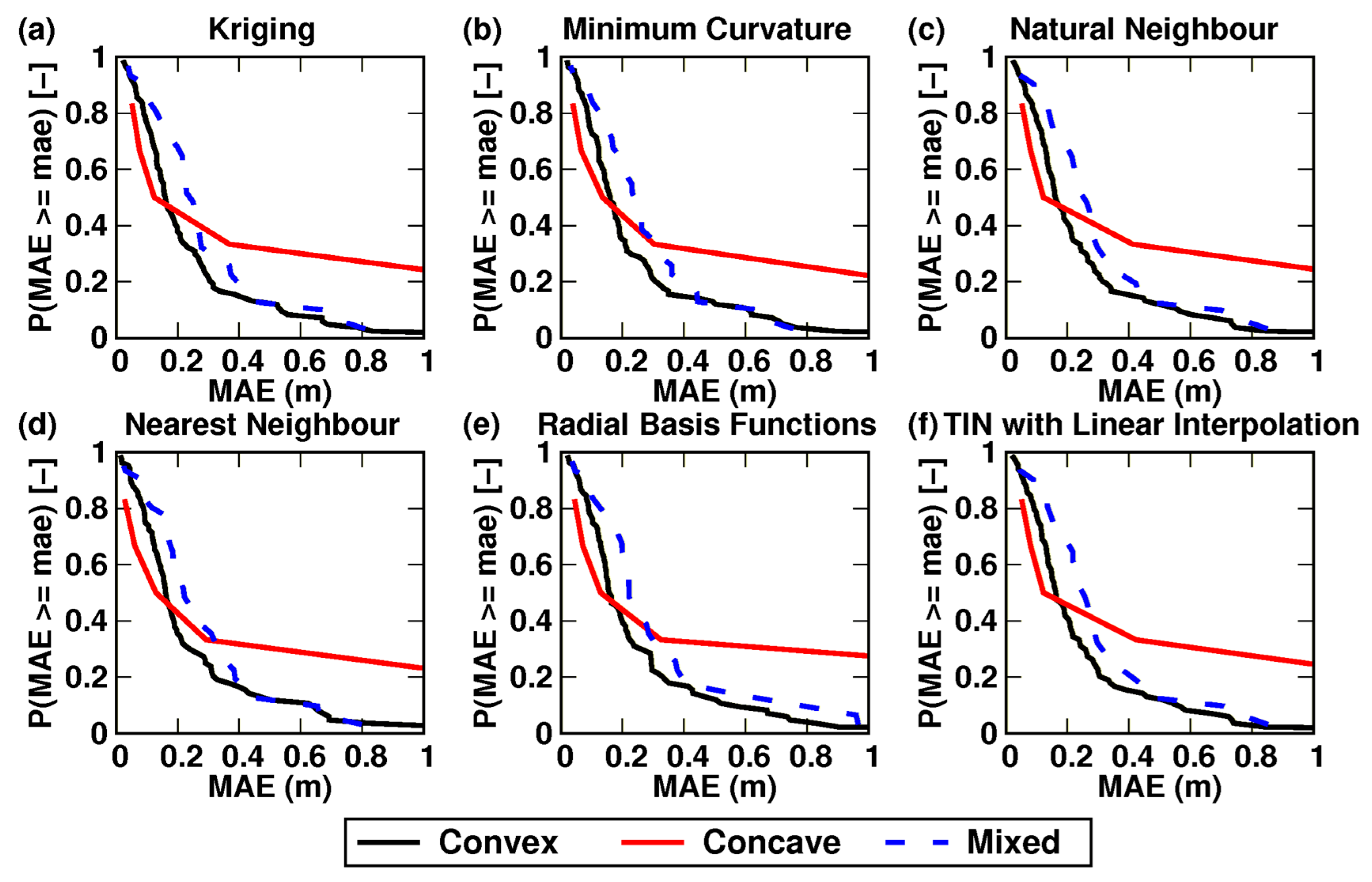
Finally, Figure 9 shows the results of the assessment that explored the accuracy of the six better-performing interpolation methods modelling the average lake forms (i.e., convex, concave, and mixed), which are characterised by different spatial (i.e., geomorphological) patterns. In the referred figure, the shape of the empirical exceedance probability distribution of the MAE for the concave lake form is not that sharp because it is defined only by 5% of the study lakes. The corresponding distributions of convex and mixed lake forms are much sharper since they are defined, respectively, by 70% and 25% of the study lakes. Despite this sharpness difference, the respective exceedance probability distributions suggest that, in general, all the methods model lakes with convex and mixed average forms similarly. All the methods seem to have a bit more trouble modelling concave patterns.
3.4. Incorporating the Lake Bathymetry into the Digital Elevation Model (DEM) of the Study Site
The product of the process for incorporating the bathymetry of the study lakes into the original DEM of the SIGTIERRAS project is an enhanced representation of the terrain of the study site, that could be very useful for the geomorphological/ecological management of the lake district of the CNP.
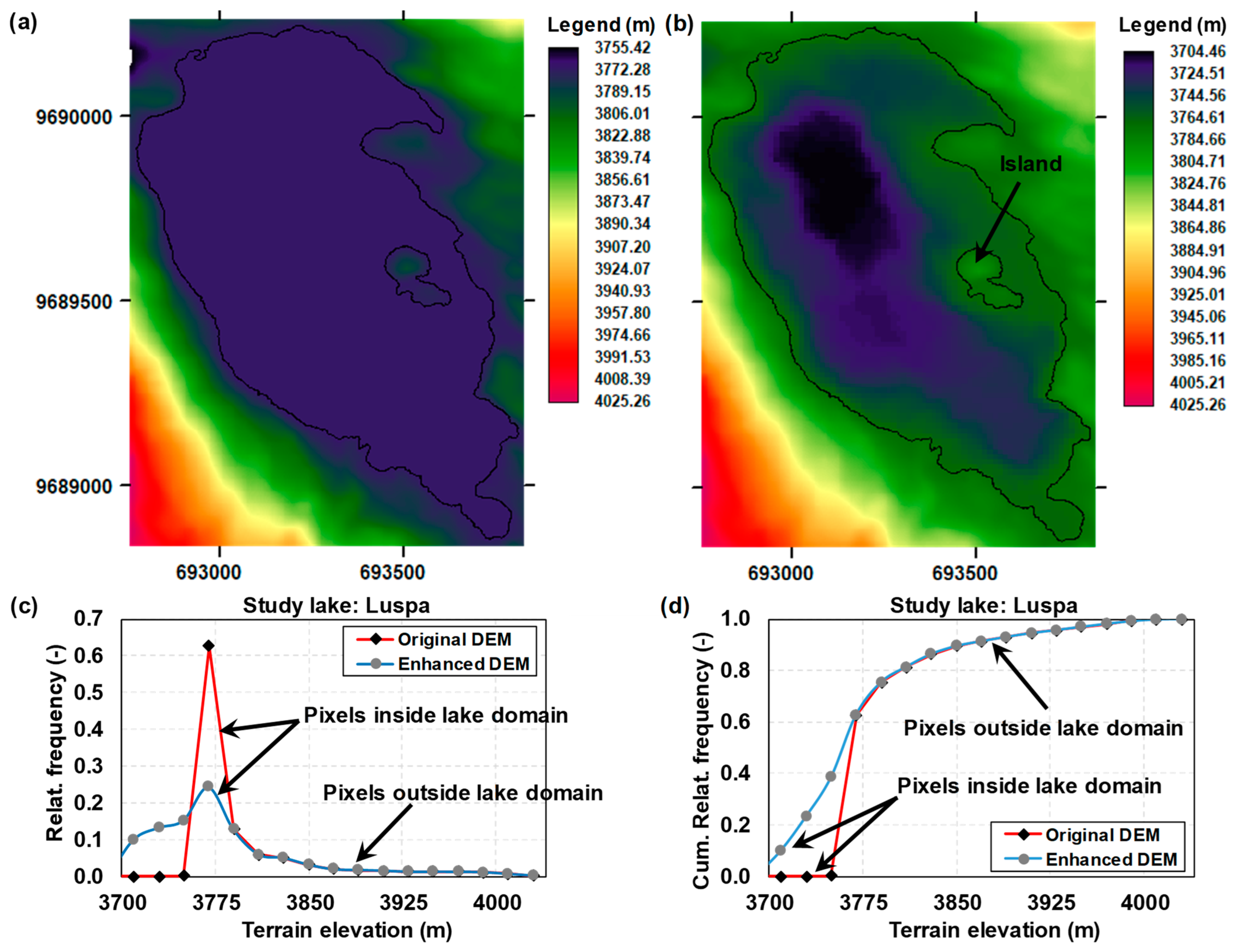
Further, the enhancement of the terrain representation of the study site is illustrated in Figure 10 for one of the study lakes: Luspa. Hereafter, Figure 10a,b depict a comparison of the DEM representation before and after the incorporation of the bathymetry of lake Luspa into the original SIGTIERRAS DEM. The discrepancy of both DEM products within the lake’s domain is clear, which means that the elevation range (see the legend in the respective figure) in the enhanced DEM is wider because lower submerged terrain levels (i.e., bathymetry) are present in it (which were not in the original DEM). Both the relative frequency and the cumulative relative frequency plots (Figure 10c,d) emphasise the important difference of both DEM products within the lake’s domain and that, outside this domain (in the depicted DEM domain), both DEM products are exactly the same, implying that the original elevations were preserved outside the study lakes.
4. Discussion
4.1. Bathymetric Surveying
A non-conventional non-specialised fishing echo-sounder system was used in this research to collect bathymetric observations. Although this specific instrument is successfully used worldwide for recreational navigation and for bathymetric surveying, there are not many examples of prior bathymetric (scientific) applications of this type of fishing echo-sounder system [12,17,56,57,58]. Consequently, there is not much information on typical measurement accuracies achieved with this type of echo-sounder fishing system which is in opposition to what happens in the case of the (combined) use of specialised instruments in the context of seabed bathymetries (see, for instance, [59,60]). This information was even more scarce when the field surveying took place, except [57] that, despite being dedicated to evaluating one of these low-cost fishing echo-sounder systems, does not provide any data on measurement accuracy. Further, no additional accurate information nor other specialised and accurate instruments were available for an accurate and detailed estimation of random measurement errors associated to the use of this particular Humminbird® echo-sounder.
Therefore, a very simple approach was adopted for estimating these errors, which produced estimates in the range 15 to 47 cm for a depth range reaching approximately 70 m. This error range seems in agreement with Yamasaki, Tabusa, Iwasaki, and Hiramatsu [56] who report a measurement error of +20 cm for a depth of 32 m (measured accurately under controlled conditions) for two combinations of echo-sounders, which were slightly more specialised than the one used in this study. On the other hand, Alcocer, Oseguera, Sánchez, González, Martínez, and González [12] report unclear manufacturer’s data, i.e., “the depth sounder has a precision of 95%”. Assuming that it implies an error of 5%, then, for depths around 70 m, they would have obtained random measurement errors around ±350 cm, which is by far higher than the magnitude of the maximum errors that were estimated in this study. Other relatively recent studies [17,58] do not provide any related information. Some manufacturers, for instance, OVA®, claim accuracies in the order of ±1% (https://www.saiyangmarine.com/depth-and-fish-finders/depth-finder/dual-frequency-echo-sounder.html; accessed on 15 January 2024), which for depths around 70 m would imply random measurement errors in the order of ±70 cm; however, no depth-differentiated accuracies are generally provided by the few manufacturers that give any related information.
Apparently, the order of magnitude of the random measurement errors that were estimated in this study is congruent with respect to the data provided by the few related studies. Nevertheless, the lack of abundant information on typical measurement accuracies when using these low-cost fishing echo-sounders to which our estimated error range could be compared is clear. This aspect was the principal reason for implementing the sensitivity analysis (SA) of the effect of the magnitude of random measurement errors on the accuracy of the interpolation methods. However, it should be stated that further limnimetric studies (for instance settling down sediment tramps and other instruments and sensors) carried out in some of these study lakes, at certain locations of interest (such as the deepest point), have revealed congruencies with the respective sonar readings with error magnitudes even lower than 17 cm. This has even accentuated the confidence on the performance that this type of fishing echo-sounders could reach in lake bathymetric studies, carried out carefully, as in the current case.
4.2. Bathymetric Modelling
The accuracy of bathymetric modelling depends, besides terrain characteristics, modelling (spatial) resolution, and the accuracy, density, and distribution of sample observations, on the interpolation method being considered [20,21,23,61]. Correspondingly, several interpolation methods (11) were tried out in the current study. This is in line with past research [20], which was carried out in the context of assessing the effect of DEM accuracy on distributed, physically based, hydrological modelling. The current study was carried out to select the best interpolation method(s) suiting the morphological characteristics of the study lakes as well as the accuracy, density, and distribution of the respective bathymetric observations, so that the best possible interpolated bathymetric products could be used in posterior studies, such as [3].
The assessment of interpolation methods has been extensively carried out in the past in the scope of surface terrain shape and roughness modelling [20,22,23,24,25,38,47,61]. There are also some assessments related to the bathymetric modelling of river and sea floors [39,40,44]. However, there are fewer assessments in the context of lake bathymetry [15,16,62], as, commonly, interpolation methods are applied on the basis of their “reputation” and/or the availability of software for their application [12,15,16,17,63] which might be considered as being “controversial”. Independently of the scope of the analyses, past assessments, with the exception of [38], have considered a lower number of methods, most of which were also used in this study. In addition, commonly, past assessments fixed their attention only on a few study sites [12,23,24,25,39,40,41,61], whilst we considered 119 study sites, which is another non-conventional aspect of our research. Some studies have even considered very few control points per study site [23,25]. Further, prior studies have concentrated on assessing the performance of some interpolation methods but using some artificial “observations” generated by test functions [41], which facilitated the optimisation of the accuracy, density, and distribution of these observations; an aspect that differs from studies such as ours that rely on real-world sample observations, acquired with low-cost instruments.
The accuracy analysis of the interpolation methods was particularly based on the consideration of some statistical measures; it was less dependent on visual comparison of their products. Therefore, it differs from some past related studies that relied mainly on visual comparison of the products of the used interpolation methods (i.e., [15,23,25]). The use of exceedance probability distributions, which is not a common approach in similar studies, proved to be a very simple but effective approach to assess the accuracy of the eleven tried methods, for all the 119 study lakes, which otherwise is commonly performed through the complicated use of several (11) plots instead of a single plot as in the current case (see, for instance, [64]). Although a very simple statistic was used in this assessment, i.e., the MAE, any other more elaborate statistic may be used, such as the root mean square error (RMSE) [L] or the relative RMSE (RRMSE) [−] or the Nash and Sutcliffe coefficient of efficiency (EF2) [−] or the Kling–Gupta efficiency (KGE) [−], or the total DEM error [L], etc., that, besides the average systematic error, can also measure the (average) random error [45,49,65] (or even much simpler statistics as in [39]). Nevertheless, although these results are not shown in this manuscript, the probability distributions derived by using some of these alternative statistics led to exactly the same conclusions as when using the MAE statistic. The plotting position method, very common in meteorological and hydrological studies [20,52,66], and easy to compute/program, proved to be an efficient tool for estimating the probability distributions of the interpolation methods; further, no perceptible differences were observed when methods other than Weibull were used (see Figure 5). Finally, notwithstanding the usefulness of the applied approach to depict the accuracy of the tried interpolation methods, in this type of assessment, it would be advisable to carry out a complementary analysis to investigate on whether bathymetric residuals are clustered and, if so, where those clusters are located within every study bathymetric domain. This could be achieved through either error maps or suitable distributed error indexes [47] or their conjunctive use. This analysis, however, is beyond the reach of this manuscript, as this complementary analysis would demand a significant amount of programming efforts to cope with the high amount of interpolation methods and study sites considered in this study.
The (bathymetric) modelling accuracy assessment indicated that the products of the methods of Kriging (ordinary), minimum curvature, multiquadric (a radial basis function), and TIN with linear interpolation and the neighbourhood methods natural neighbour and nearest neighbour were better than the rest, with the exception of the other two neighbourhood methods of modified Shepard’s and inverse distance (IDW), whose accuracy was not that much inferior and even outperformed the respective accuracies of more elaborate methods such as polynomial regression. Indeed, this study revealed an equivalence of the six better-performing methods, as no single “best” interpolation method could be identified among them for our study conditions (i.e., lake geomorphological and data characteristics). These aspects are somewhat consistent with what similar studies reported (i.e., [25,61]) in the sense that, although a best method was identified, the performance of other, less sophisticated methods, such as IDW, was not that inferior. Particularly because of its ability to adjust itself to the spatial structure of the observations, Kriging (or other sophisticated methods such as spline) is normally chosen as the best interpolation method [23,24,25,39,43], although some studies revealed that even simpler neighbourhood methods such as IDW performed similarly or even outperformed Kriging (and/or spline) [26,28,45,61]. All the above emphasise the need for carrying out an inspection of the performance/accuracy of the candidate interpolation methods, similarly to what has been performed in this study, so that the best possible bathymetric products are obtained for the study beforehand; the more sophisticated methods are not always the best choice for local geomorphological and observed data conditions.
Conventional random sampling took place in the scope of a split-sample (SS) test for training the interpolation methods and evaluating (i.e., “validating”) the accuracy of their products. Hereafter, several data densities were tried out to cross-check the congruency of the accuracy assessments (see Figure 5 for an example of the tried densities). The assessment indicated an important congruency of results, despite the fact that the sharpness of the empirical exceedance probability distributions was reduced for lower data densities. Other similar research also studied the effects of data density variability on the interpolation methods [23,24,40,61], usually through a similar SS test. However, it is rarely addressed in these studies that, independently of the data density beforehand, conventional random sampling may lead (by chance) to leaving key data out of the interpolation process. This may affect the ability of the respective interpolated product to represent certain important spatial patterns present in reality well. There is the chance, however, that through the repetition of the analysis, conventional random sampling would include these key data in the interpolation process, resulting in a higher accuracy evaluation for the same data density and interpolation method. This is, definitively, a potential small pitfall of conventional random sampling in an SS test.
To overcome it, cluster random sampling might be applied if prior knowledge of particular spatial patterns is available, which could be perfectly feasible for ground topography studies; nevertheless, this is not a common option when dealing with bathymetric studies as the inundated surface being modelled is normally imperceptible to the eye. But even if it were feasible in normal bathymetric studies, there would be still a chance that some of the key data would be left out of the interpolation process given that, within every cluster, sampling would still be fully random. A different alternative (cross-validation) would be leaving one observation out of the interpolation process at a time and then evaluating the accuracy of the interpolated product against that particular observation. This process should be repeated as many times as needed so that all depth measurements are omitted once (so, using all the available observations for comparison, and using nearly all the observations in the interpolation); after which an average accuracy measure could be obtained for the tried density and interpolation method upon the whole set of repetitions [47]. Nevertheless, this would be difficult to achieve for studies that handle a large number of observations, such as in the current case. What has been performed in this study, for a given data density and interpolation method, is repeating the respective SS test several times (an approach that was also adopted by [40], though with a different purpose in mind) and cross-checking the congruency of the corresponding results/findings. This kind of sensitivity analysis (SA) revealed an important degree of congruency; however, very few repetitions of the SS test led to lower accuracies (for a given data density and interpolation method), emphasising potential pitfall of the random data selection in the context of the SS test.
The SA of the effect of the magnitude of random measurement errors on the accuracy of the interpolation methods suggested that, given the morphological conditions of the study lakes and the properties of the bathymetric observations (the acceptable density and proximity), the consideration of even higher error magnitudes than the ones estimated in this study leads to the same results obtained before the SA took place, confirming, therefore, the same six better-performing interpolation methods. The SA also supported the assumption, implicit in this study, that data proximity is a very important aspect for the performance of interpolation methods; at least, it is as important as random measurement errors of reasonable magnitudes present in the observations.
In this regard, random measurement errors were not filtered out from the original bathymetric observations, particularly to represent real-word management practices, but also because it is beyond the scope of the current manuscript. Further, any numerical filtering of the bathymetric observations would result in a data set whose bathymetric accuracy enhancement could not be proved unless very accurate bathymetric data sets are available at least for some of the study lakes to contrast the validity of the filtering products. As already stated, this accurate bathymetric data set was not available in this research; nor was it available in the context of a real-world management study aiming at producing bathymetric models under low-budget conditions, as in the current case. Instead, the low-pass Gaussian filter was applied on the interpolated products prior to the evaluation phase with the aim of smoothing the interpolation products and eliminating potential artificial features (for instance, pitholes) introduced by the interpolation methods.
It should be noticed that none of the research studies that have applied, recently, fishing echo-sounder systems for surveying lake bathymetry (i.e., [12,17]) have performed the estimation of random measurement errors, filtering of these random errors from the observations, application of a smoothing filter on the bathymetric surfaces after interpolation, or a similar SA to the one implemented in this study. Thus, the different analyses implemented in this study are believed to have supported the reliability of its results.
4.3. Incorporating the Lake Bathymetry into the Digital Elevation Model (DEM) of the Study Site
The resulting bathymetric products were incorporated into the best DEM of the study area, which lacks bathymetric information. This, undoubtedly, improved the information provided by the DEM. A couple of aspects have to be considered, however. The first one has to do with the difference in terms of the accuracy and density of information between the current sonar-based surveying and the respective LiDAR-based surveying by which the (SIGTIERRAS) DEM was generated. Another aspect has to do with the difference in terms of interpolation method and resolution that were applied in the current study and the study that produced the SIGTIERRAS DEM. These aspects produced, possibly, bathymetric products of inferior accuracy and resolution with respect to the SIGTIERRAS DEM. This not uncommon in studies where, similarly to what happened in the current research, digital elevation products resulting from different data gathering and interpolation approaches were integrated [40,67].
In this study, an initial, very simple integration approach was followed to (i) match the resolution of both elevation products by resampling the original bathymetric surfaces according to the resolution of the DEM and (ii) equalise the elevation references of the bathymetries with the respective reference of the DEM by assigning a DEM-based elevation to the perimeters considered in the interpolation of the study lakes. In this regard, although more complex approaches could be applied depending on the nature of the information to be integrated, for instance, correlating certain statistical properties of both elevation data sets [67], they are generally based, as in our case, on equalising the elevation references of both data sets (bathymetry and the lake’s surrounding topography).
4.4. Average Lake Form
The comparison of the hypsometric properties of the study lakes was facilitated through the use of relative hypsometric curves. Indeed, defining this type of standardised hypsometric curve for comparison of geomorphological features was the main purpose of pioneering research such as that by Strahler [53] for hydrological basins or Håkanson [13] for lakes. Although this concept would be perfectly applicable without mathematical constraints with regard to the (spatial) scale of analysis (i.e., to either huge or small basins) or type of geomorphological feature (i.e., to a hydrological basin or a natural lake basin or an artificial reservoir), there are some practical limitations that have to do, for instance, with the congruency of the comparison and the respective interpretation of the results. Therefore, it should be observed that the way of calculating a hypsometric curve for a hydrological basin [53] is slightly different from the way of doing so for a lake or reservoir [68]. Thus, issuing a general or a regional interpretation, for instance, for lakes, upon local assessments or the examination of geomorphological features other than lakes should be avoided when using relative hypsometric curves [13].
In this regard, our comparison was carried out among lakes that belong to the same district and that share the same glacial origin. Even though the area range of the study lakes is broad (from about 0.005 km2 to more than 0.46 km2), we believe that a single comparison, without the need for clustering the study lakes, is justifiable since our intention was simply assessing their average form and given that they share the same glacial genesis. For assessing the average form of the study lakes, we applied a simple approach [13], which enabled the relatively easy programming of the subroutines for handling the numerous necessary computations. Nevertheless, Håkanson [13] and Håkanson [14] present a more complex analysis that uses probability distributions to improve the assessment, which also enabled considering more lake form categories than the ones used in this study. Our intention was not trying to link any potential cause, such as erosion/deposition rates, with differences in terms of average form. In this context, Kim, Kim, Wang, Lee, and Kim [68] have directly applied an approach, originally developed by Strahler [53] to address the geological maturity of hydrological basins, on some reservoirs’ bathymetric data to conclude on their degree of erosion after using relative hypsometric curves. Although this might be (weakly) acceptable for artificial reservoirs, this approach would be controversial for natural lakes because of the reasons described above.
The assessment on the accuracy of the six better-performing interpolation methods modelling the inherent different spatial patterns of the three average lake forms confirmed not only the equivalence of the products of these methods but also the fact that, for instance, for the bigger lake form groups, i.e., convex and mixed, simpler neighbourhood methods such as nearest neighbour performed comparably to more sophisticated methods such as Kriging (ordinary) and even slightly outperformed it for some of the study lakes (Figure 9a,d). Further, all the inspected methods produced less accurate products for lakes with average concave forms. Thus, this inherent spatial pattern analysis did not shed more light onto the process of identifying an undebatable “best” interpolation method for our study conditions. This also confirmed that sophisticated interpolation methods do not always produce the best products; geomorphological characteristics of the study site(s) together with observation data characteristics play an important role in the performance of the methods.
The knowledge of the bathymetry of lakes can help in defining important geomorphological parameters such as volume, shape, or residence time, which are very important for ecological processes and interactions with the environment [69] such as influencing primary productivity [70], food web dynamics [71], or species diversity [72]. However, in the CNP there is not yet published research that links ecological processes and geomorphology since relevant research has taken place there only in the last ten years. The results of the current manuscript fall into the “knowledge pieces” about these unique ecosystems and could contribute to more holistic knowledge on the connection of physical–chemical–biological processes happening in these lakes. The understanding of the linkage between geomorphological characteristics and ecological processes could provide in the future sound management and policy recommendations.
5. Conclusions
A single best interpolation method could not be identified; instead, the probability distributions suggested the equivalence of six of the tried methods including the complex methods Kriging (ordinary), minimum curvature (spline), multiquadric (a radial basis function), and TIN with linear interpolation but also the much simpler neighbourhood methods natural neighbour and nearest neighbour. The implemented SA confirmed this. This suggested that sophisticated interpolation methods do not always produce the best products; geomorphological characteristics of the study site(s) together with observation data characteristics (particularly, proximity and accuracy) are likely to play important roles in their performance. As such, this type of assessment should be carried out in any terrestrial mapping of bathymetry that is based on the interpolation of scattered observations. Further, the accuracy analysis as a function of the three average form categories (i.e., convex, concave, and mixed) did not help to elucidate an undebatable best interpolation method.
Finally, it is believed that the enhanced DEM resulting from the incorporation of the interpolated bathymetries of 114 of the study lakes into the best DEM of the study site could be a very useful tool for a more appropriate management of this very fragile high mountain tropical lake district of southern Ecuador. This is despite the accuracy difference of the data sets (i.e., lake bathymetries and existing DEM).
Future work could include the use of remote sensing information to model the bathymetry of these lakes so that non-terrestrial approaches could be used within acceptable uncertainty constraints without the need for physically and financially demanding activities. Other future activities may include applying the main findings of this research to ecological or hydrological modelling or exploring the impact of climate change on the physical behaviour of the study lakes, etc.
Author Contributions
Conceptualisation, R.F.V., P.V.M. and H.H.; methodology, R.F.V., P.V.M. and H.H.; software, R.F.V.; validation, R.F.V., P.V.M. and H.H.; formal analysis, R.F.V. and P.V.M.; investigation, R.F.V., P.V.M. and H.H.; resources, P.V.M., R.F.V. and H.H.; data curation, P.V.M. and R.F.V.; writing—original draft preparation, R.F.V. and H.H.; writing—review and editing, R.F.V., H.H. and P.V.M.; visualisation, R.F.V.; supervision, R.F.V. and H.H.; project administration, H.H. and R.F.V.; funding acquisition, R.F.V., P.V.M. and H.H. All authors have read and agreed to the published version of the manuscript.
Funding
This research was partially funded by the Research Directorate of the University of Cuenca (DIUC) and the Municipal Public Enterprise of Telecommunications, Drinking Water, Sewage and Sanitation of Cuenca (ETAPA EP). The APC was funded by the Vice-presidency of Research of the University of Cuenca (VIUC).
Data Availability Statement
Restrictions apply to the availability of data used in this research. Observation data were acquired by the authors belonging to both financing institutions. The number of surveyed lakes exceeded by far the expected number initially considered in the research project “Caracterización limnológica de los lagos y lagunas del Parque Nacional Cajas”, for which very little financial support was available. Most of the field and office work was carried out in the free time of the researchers.
Conflicts of Interest
The authors declare no conflicts of interest. The funders had no role in the design of the study; in the collection, analyses, or interpretation of data; in the writing of the manuscript; or in the decision to publish the results.
References
- Viviroli, D.; Kummu, M.; Meybeck, M.; Kallio, M.; Wada, Y. Increasing dependence of lowland populations on mountain water resources. Nat. Sustain. 2020, 3, 917–928. [Google Scholar] [CrossRef]
- Grêt-Regamey, A.; Brunner, S.H.; Kienast, F. Mountain Ecosystem Services: Who Cares? Mt. Res. Dev. 2012, 32, S24–S34. [Google Scholar] [CrossRef]
- Mosquera, P.V.; Hampel, H.; Vázquez, R.F.; Alonso, M.; Catalan, J. Abundance and morphometry changes across the high-mountain lake-size gradient in the tropical Andes of Southern Ecuador. Water Resour. Res. 2017, 53, 7269–7280. [Google Scholar] [CrossRef]
- Mosquera, P.V.; Hampel, H.; Vázquez, R.F.; Catalan, J. Water chemistry variation in tropical high-mountain lakes on old volcanic bedrocks. Limnol. Oceanogr. 2022, 67, 1522–1536. [Google Scholar] [CrossRef]
- Giles, M.P.; Michelutti, N.; Grooms, C.; Smol, J.P. Long-term limnological changes in the Ecuadorian páramo: Comparing the ecological responses to climate warming of shallow waterbodies versus deep lakes. Freshw. Biol. 2018, 63, 1316–1325. [Google Scholar] [CrossRef]
- Michelutti, N.; Wolfe, A.P.; Cooke, C.A.; Hobbs, W.O.; Vuille, M.; Smol, J.P. Climate Change Forces New Ecological States in Tropical Andean Lakes. PLoS ONE 2015, 10, e0115338. [Google Scholar] [CrossRef] [PubMed]
- Catalán, J.; Donato Rondón, J.C. Perspectives for an integrated understanding of tropical and temperate high-mountain lakes. J. Limnol. 2016, 75, 215–234. [Google Scholar] [CrossRef]
- Woolway, R.I.; Kraemer, B.M.; Lenters, J.D.; Merchant, C.J.; O’Reilly, C.M.; Sharma, S. Global lake responses to climate change. Nat. Rev. Earth Environ. 2020, 1, 388–403. [Google Scholar] [CrossRef]
- Palomino-Ángel, S.; Vázquez, R.F.; Hampel, H.; Anaya, J.A.; Mosquera, P.V.; Lyon, S.W.; Jaramillo, F. Retrieval of Simultaneous Water-Level Changes in Small Lakes with InSAR. Geophys. Res. Lett. 2022, 49, e2021GL095950. [Google Scholar] [CrossRef]
- Luethje, M.; Mosquera, P.V.; Hampel, H.; Fritz, S.C.; Benito, X. Planktic diatom responses to spatiotemporal environmental variation in high-mountain tropical lakes. Freshw. Biol. 2024, 69, 387–402. [Google Scholar] [CrossRef]
- Prigent, C.; Papa, F.; Aires, F.; Jimenez, C.; Rossow, W.B.; Matthews, E. Changes in land surface water dynamics since the 1990s and relation to population pressure. Geophys. Res. Lett. 2012, 39, L08403. [Google Scholar] [CrossRef]
- Alcocer, J.; Oseguera, L.A.; Sánchez, G.; González, C.G.; Martínez, J.R.; González, R. Bathymetric and morphometric surveys of the Montebello Lakes, Chiapas. J. Limnol. 2016, 75, 56–65. [Google Scholar] [CrossRef]
- Håkanson, L. On Lake Form, Lake Volume and Lake Hypsographic Survey. Geogr. Annaler. Ser. A Phys. Geogr. 1977, 59, 1–30. [Google Scholar] [CrossRef]
- Håkanson, L. Optimization of lake hydrographic surveys. Water Resour. Res. 1978, 14, 545–560. [Google Scholar] [CrossRef]
- De Maisonneuve, C.B.; Eisele, S.; Forni, F.; Hamdi; Park, E.; Phua, M.; Putra, R. Bathymetric survey of lakes Maninjau and Diatas (West Sumatra), and lake Kerinci (Jambi). J. Phys. Conf. Ser. 2019, 1185, 012001. [Google Scholar] [CrossRef]
- Gonçalves, M.A.; Garcia, F.C.; Barroso, G.F. Morphometry and mixing regime of a tropical lake: Lake Nova (Southeastern Brazil). An. Acad. Bras. Ciências 2016, 88, 1341–1356. [Google Scholar] [CrossRef] [PubMed]
- Van Colen, W.; Portilla, K.; Oña, T.; Wyseure, G.; Goethals, P.; Velarde, E.; Muylaert, K. Limnology of the neotropical high elevation shallow lake Yahuarcocha (Ecuador) and challenges for managing eutrophication using biomanipulation. Limnologica 2017, 67, 37–44. [Google Scholar] [CrossRef]
- Gholamalifard, M.; Kutser, T.; Esmaili-Sari, A.; Abkar, A.A.; Naimi, B. Remotely Sensed Empirical Modeling of Bathymetry in the Southeastern Caspian Sea. Remote Sens. 2013, 5, 2746–2762. [Google Scholar] [CrossRef]
- Pope, A.; Scambos, T.A.; Moussavi, M.; Tedesco, M.; Willis, M.; Shean, D.; Grigsby, S. Estimating supraglacial lake depth in West Greenland using Landsat 8 and comparison with other multispectral methods. Cryosphere 2016, 10, 15–27. [Google Scholar] [CrossRef]
- Vázquez, R.F.; Feyen, J. Assessment of the effects of DEM gridding on the predictions of basin runoff using MIKE SHE and a modelling resolution of 600 m. J. Hydrol. 2007, 334, 73–87. [Google Scholar] [CrossRef]
- Vivoni, E.R.; Ivanov, V.Y.; Bras, R.L.; Entekhabi, D. On the effects of triangulated terrain resolution on distributed hydrologic model response. Hydrol. Process. 2005, 19, 2101–2122. [Google Scholar] [CrossRef]
- Guo, Q.; Li, W.; Yu, H.; Alvarez, O. Effects of Topographic Variability and Lidar Sampling Density on Several DEM Interpolation Methods. Photogramm. Eng. Remote Sens. 2010, 76, 701–712. [Google Scholar] [CrossRef]
- Chu, H.-J.; Wang, C.-K.; Huang, M.-L.; Lee, C.-C.; Liu, C.-Y.; Lin, C.-C. Effect of point density and interpolation of LiDAR-derived high-resolution DEMs on landscape scarp identification. GISci. Remote Sens. 2014, 51, 731–747. [Google Scholar] [CrossRef]
- Chen, C.; Bei, Y.; Li, Y.; Zhou, W. Effect of interpolation methods on quantifying terrain surface roughness under different data densities. Geomorphology 2022, 417, 108448. [Google Scholar] [CrossRef]
- Arun, P.V. A comparative analysis of different DEM interpolation methods. Egypt. J. Remote Sens. Space Sci. 2013, 16, 133–139. [Google Scholar] [CrossRef]
- Boke, A. Comparative Evaluation of Spatial Interpolation Methods for Estimation of Missing Meteorological Variables over Ethiopia. J. Water Resour. Prot. 2017, 9, 945–959. [Google Scholar] [CrossRef]
- Keskin, M.; Dogru, A.O.; Balcik, F.B.; Goksel, C.; Ulugtekin, N.; Sozen, S. Comparing Spatial Interpolation Methods for Mapping Meteorological Data in Turkey. In Energy Systems and Management; Springer: Cham, Switzerland, 2015; pp. 33–42. [Google Scholar]
- Declercq, F.A.N. Interpolation Methods for Scattered Sample Data: Accuracy, Spatial Patterns, Processing Time. Cartogr. Geogr. Inf. Syst. 1996, 23, 128–144. [Google Scholar] [CrossRef]
- Chiang, W.H. Processing Modflow, An Integrated Modeling Environment for the Simulation of Groundwater Flow, Transport and Reactive Processes. In Users Manual, Manuscript, Simcore Software; Simcore: Halifax, UK, 2012; p. 484. [Google Scholar]
- Holzbecher, E. Environmental Modeling Using MATLAB; Springer: Berlin/Heidelberg, Germany, 2007. [Google Scholar]
- Hungerbühler, D.; Steinmann, M.; Winkler, W.; Seward, D.; Egüez, A.; Peterson, D.E.; Helg, U.; Hammer, C. Neogene stratigraphy and Andean geodynamics of southern Ecuador. Earth-Sci. Rev. 2002, 57, 75–124. [Google Scholar] [CrossRef]
- Hansen, B.C.S.; Rodbell, D.T.; Seltzer, G.O.; León, B.; Young, K.R.; Abbott, M. Late-glacial and Holocene vegetational history from two sites in the western Cordillera of southwestern Ecuador. Palaeogeogr. Palaeoclimatol. Palaeoecol. 2003, 194, 79–108. [Google Scholar] [CrossRef]
- Colinvaux, P.A.; Bush, M.B.; Steinitz-Kannan, M.; Miller, M.C. Glacial and Postglacial Pollen Records from the Ecuadorian Andes and Amazon. Quat. Res. 1997, 48, 69–78. [Google Scholar] [CrossRef]
- Ramsay, P.M.; Oxley, E.R.B. The growth form composition of plant communities in the ecuadorian páramos. Plant Ecol. 1997, 131, 173–192. [Google Scholar] [CrossRef]
- Alvites, C.; Battipaglia, G.; Santopuoli, G.; Hampel, H.; Vázquez, R.F.; Matteucci, G.; Tognetti, R.; De Micco, V. Dendrochronological analysis and growth patterns of Polylepis reticulata (Rosaceae) in the Ecuadorian Andes. IAWA J. 2019, 40, S331–S335. [Google Scholar] [CrossRef]
- Davis, J.C. Statistics and Data Analysis in Geology; John Wiley and Sons: New York, NY, USA, 2002; p. 638. [Google Scholar]
- Humminbird. Humminbird Operations Manual 1198c SI Combo; Humminbird: Eufaula, AL, USA, 2012; p. 207. [Google Scholar]
- Yang, C.-S.; Kao, S.-P.; Lee, F.-B.; Hung, P.-S. Twelve different interpolation methods: A case study of Surfer 8.0. In Proceedings of the XXth ISPRS Congress “Geo-Imagery Bridging Continents”, Istanbul, Turkey, 12–23 July 2004; pp. 778–785. [Google Scholar]
- Aykut, N.O.; Akpınar, B.; Aydın, Ö. Hydrographic data modeling methods for determining precise seafloor topography. Comput. Geosci. 2013, 17, 661–669. [Google Scholar] [CrossRef]
- Amante, C.J.; Eakins, B.W. Accuracy of Interpolated Bathymetry in Digital Elevation Models. J. Coast. Res. 2016, 76, 123–133. [Google Scholar] [CrossRef]
- Franke, R.; Nielson, G. Smooth interpolation of large sets of scattered data. Int. J. Numer. Methods Eng. 1980, 15, 1691–1704. [Google Scholar] [CrossRef]
- Renka, R.J. Algorithm 660: QSHEP2D: Quadratic Shepard Method for Bivariate Interpolation of Scattered Data. ACM Trans. Math. Softw. 1988, 14, 149–150. [Google Scholar] [CrossRef]
- Eldrandaly, K.A.; Abu-Zaid, M.S. Comparison of Six GIS-Based Spatial Interpolation Methods for Estimating Air Temperature in Western Saudi Arabia. J. Environ. Inform. 2011, 18, 38–45. [Google Scholar] [CrossRef]
- Merwade, V.M.; Maidment, D.R.; Goff, J.A. Anisotropic considerations while interpolating river channel bathymetry. J. Hydrol. 2006, 331, 731–741. [Google Scholar] [CrossRef]
- Li, L.; Nearing, M.A.; Nichols, M.H.; Polyakov, V.O.; Phillip Guertin, D.; Cavanaugh, M.L. The effects of DEM interpolation on quantifying soil surface roughness using terrestrial LiDAR. Soil Tillage Res. 2020, 198, 104520. [Google Scholar] [CrossRef]
- Pannatier, Y. VARIOWIN Software for Spatial Data Analysis in 2D; Springer: New York, NY, USA, 1996; p. 91. [Google Scholar]
- Erdogan, S. A comparision of interpolation methods for producing digital elevation models at the field scale. Earth Surf. Process. Landf. 2009, 34, 366–376. [Google Scholar] [CrossRef]
- Franke, R. Smooth interpolation of scattered data by local thin plate splines. Comput. Math. Appl. 1982, 8, 273–281. [Google Scholar] [CrossRef]
- Vázquez, R.F.; Brito, J.E.; Hampel, H.; Birkinshaw, S. Assessing the Performance of SHETRAN Simulating a Geologically Complex Catchment. Water 2022, 14, 3334. [Google Scholar] [CrossRef]
- Wei, C.; Zhao, Q.; Lu, Y.; Fu, D. Assessment of Empirical Algorithms for Shallow Water Bathymetry Using Multi-Spectral Imagery of Pearl River Delta Coast, China. Remote Sens. 2021, 13, 3123. [Google Scholar] [CrossRef]
- Hassan, M.H.; Nadaoka, K. Assessment of machine learning approaches for bathymetry mapping in shallow water environments using multispectral satellite images. Int. J. Geoinform. 2017, 13, 1–15. [Google Scholar]
- Hong, H.P.; Li, S.H. Plotting positions and approximating first two moments of order statistics for Gumbel distribution: Estimating quantiles of wind speed. Wind Struct. 2014, 19, 371–387. [Google Scholar] [CrossRef]
- Strahler, A.N. Hypsometric (Area-Altitude) Analysis of Erosional Topography. GSA Bull. 1952, 63, 1117–1142. [Google Scholar] [CrossRef]
- Langbein, W.B. Topographic Characteristics of Drainage Basins; 968C; United States Department of the Interior, Geological Survey: Reston, VA, USA, 1947; pp. 125–158.
- Franke, R. Scattered data interpolation: Tests of some methods. Math. Comput. 1982, 38, 181–200. [Google Scholar]
- Yamasaki, S.; Tabusa, T.; Iwasaki, S.; Hiramatsu, M. Acoustic water bottom investigation with a remotely operated watercraft survey system. Prog. Earth Planet. Sci. 2017, 4, 25. [Google Scholar] [CrossRef]
- Hatanaka, K.; Toda, M.; Wada, M. Data Analysis of a Low-Cost Bathymetry System Using Fishing Echo Sounders. In Proceedings of the OCEANS 2007, Vancouver, BC, Canada, 29 September–4 October 2007; pp. 1–6. [Google Scholar]
- Neupane, B.; Thakuri, S.; Gurung, N.; Aryal, A.; Bhandari, B.; Pathak, K. Lake Bathymetry, Morphometry and Hydrochemistry of Gosaikunda and Associated Lake. J. Tour. Himal. Adventures 2022, 4, 34–45. [Google Scholar] [CrossRef]
- Bongiovanni, C.; Stewart, H.A.; Jamieson, A.J. High-resolution multibeam sonar bathymetry of the deepest place in each ocean. Geosci. Data J. 2022, 9, 108–123. [Google Scholar] [CrossRef]
- Ernstsen, V.B.; Noormets, R.; Hebbeln, D.; Bartholomä, A.; Flemming, B.W. Precision of high-resolution multibeam echo sounding coupled with high-accuracy positioning in a shallow water coastal environment. Geo-Mar. Lett. 2006, 26, 141–149. [Google Scholar] [CrossRef]
- Aguilar, F.J.; Agüera, F.; Aguilar, M.A.; Carvajal, F. Effects of Terrain Morphology, Sampling Density, and Interpolation Methods on Grid DEM Accuracy. Photogramm. Eng. Remote Sens. 2005, 7, 805–816. [Google Scholar] [CrossRef]
- Liu, K.; Song, C.; Zhan, P.; Luo, S.; Fan, C. A Low-Cost Approach for Lake Volume Estimation on the Tibetan Plateau: Coupling the Lake Hypsometric Curve and Bottom Elevation. Front. Earth Sci. 2022, 10, 925944. [Google Scholar] [CrossRef]
- Paul, S.; Oppelstrup, J.; Thunvik, R.; Magero, J.M.; Ddumba Walakira, D.; Cvetkovic, V. Bathymetry Development and Flow Analyses Using Two-Dimensional Numerical Modeling Approach for Lake Victoria. Fluids 2019, 4, 182. [Google Scholar] [CrossRef]
- Martinsen, K.T.; Sand-Jensen, K.; Selvan, R. Predicting lake bathymetry from the topography of the surrounding terrain using deep learning. Limnol. Oceanogr. Methods 2023, 21, 625–636. [Google Scholar] [CrossRef]
- Gupta, H.V.; Kling, H.; Yilmaz, K.K.; Martinez, G.F. Decomposition of the mean squared error and NSE performance criteria: Implications for improving hydrological modelling. J. Hydrol. 2009, 377, 80–91. [Google Scholar] [CrossRef]
- Vázquez, R.F.; Beven, K.; Feyen, J. GLUE based assessment on the overall predictions of a MIKE SHE application. Water Resour. Manag. 2009, 23, 1325–1349. [Google Scholar] [CrossRef]
- Julzarika, A.; Aditya, T.; Subaryono, S.; Harintaka, H.; Dewi, R.S.; Subehi, L. Integration of the latest Digital Terrain Model (DTM) with Synthetic Aperture Radar (SAR) Bathymetry. J. Degrad. Min. Lands Manag. 2021, 8, 2759–2768. [Google Scholar] [CrossRef]
- Kim, D.; Kim, J.; Wang, W.; Lee, H.; Kim, H.S. On Hypsometric Curve and Morphological Analysis of the Collapsed Irrigation Reservoirs. Water 2022, 14, 907. [Google Scholar] [CrossRef]
- Messager, M.L.; Lehner, B.; Grill, G.; Nedeva, I.; Schmitt, O. Estimating the volume and age of water stored in global lakes using a geo-statistical approach. Nat. Commun. 2016, 7, 13603. [Google Scholar] [CrossRef]
- Staehr, P.A.; Baastrup-Spohr, L.; Sand-Jensen, K.; Stedmon, C. Lake metabolism scales with lake morphometry and catchment conditions. Aquat. Sci. 2012, 74, 155–169. [Google Scholar] [CrossRef]
- Post, D.M.; Pace, M.L.; Hairston, N.G. Ecosystem size determines food-chain length in lakes. Nature 2000, 405, 1047–1049. [Google Scholar] [CrossRef] [PubMed]
- Dodson, S.I.; Arnott, S.E.; Cottingham, K.L. The Relationship In Lake Communities between Primary Productivity and Species Richness. Ecology 2000, 81, 2662–2679. [Google Scholar] [CrossRef]
Figure 1.
Location of the study site and distribution of the study lakes. Lake identifiers (IDs) are after Mosquera, Hampel, Vázquez, Alonso, and Catalan [3]. The large majority of them (115) are located within the Cajas National Park (CNP), 3 lakes are in the Quimsacocha volcano area, and 1 (lake 157, not shown) is in the Sangay National Park (SNP). Coordinates system: Geographic.

Figure 2.
Digital elevation model (DEM) of the study site available from the Ecuadorian government’s project SIGTIERRAS (www.sigtierras.gob.ec) (a) in the form of separate pieces (tiles), each one of which has a size of 770 rows and 775 columns (with a 3 × 3 m2 resolution), which were mosaicked (b) in the context of this study. For illustration, only a few of the 217 DEM tiles are depicted in (a). For comparison purposes, the bound of the Cajas National Park (CNP) and the perimeters of the study lakes are also depicted, along with the rectangle that defines the horizontal domain considered in this study for the topography. Coordinates system: UTM (m) 17-S, WGS84.
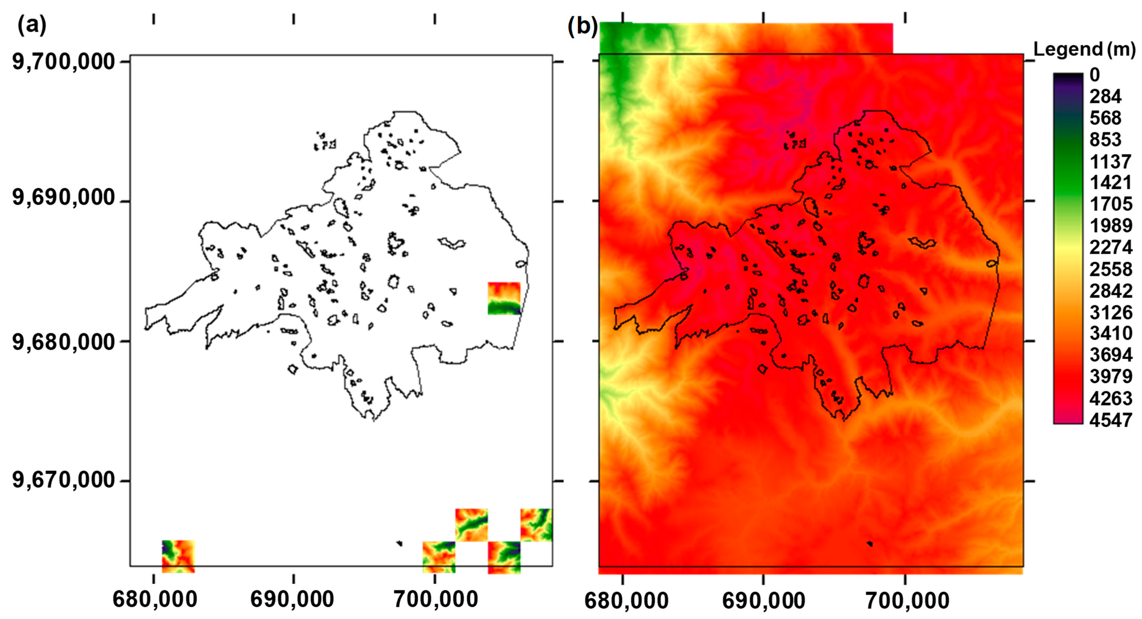
Figure 3.
Flow chart of the protocol that was followed for acquiring field observations and modelling the respective bathymetric surfaces for all of the study lakes of the Cajas National Park (CNP).
Figure 3.
Flow chart of the protocol that was followed for acquiring field observations and modelling the respective bathymetric surfaces for all of the study lakes of the Cajas National Park (CNP).

Figure 4.
(a) Random measurement errors estimated by repeatedly collecting observations in fixed spots within 5 study lakes (i.e., Llaviuco, Toreadora, Larga, Luspa, and Sunincocha Grande); (b) distribution of training (80%) and evaluation (20%) bathymetric observations in the scope of the surveying of one of the deepest study lakes, Luspa (surface area: 0.77 km2), Cajas National Park (CNP), Ecuador; and (c) the respective bathymetric product of the natural neighbour interpolation method. Coordinates system: UTM (m) 17-S, WGS84.
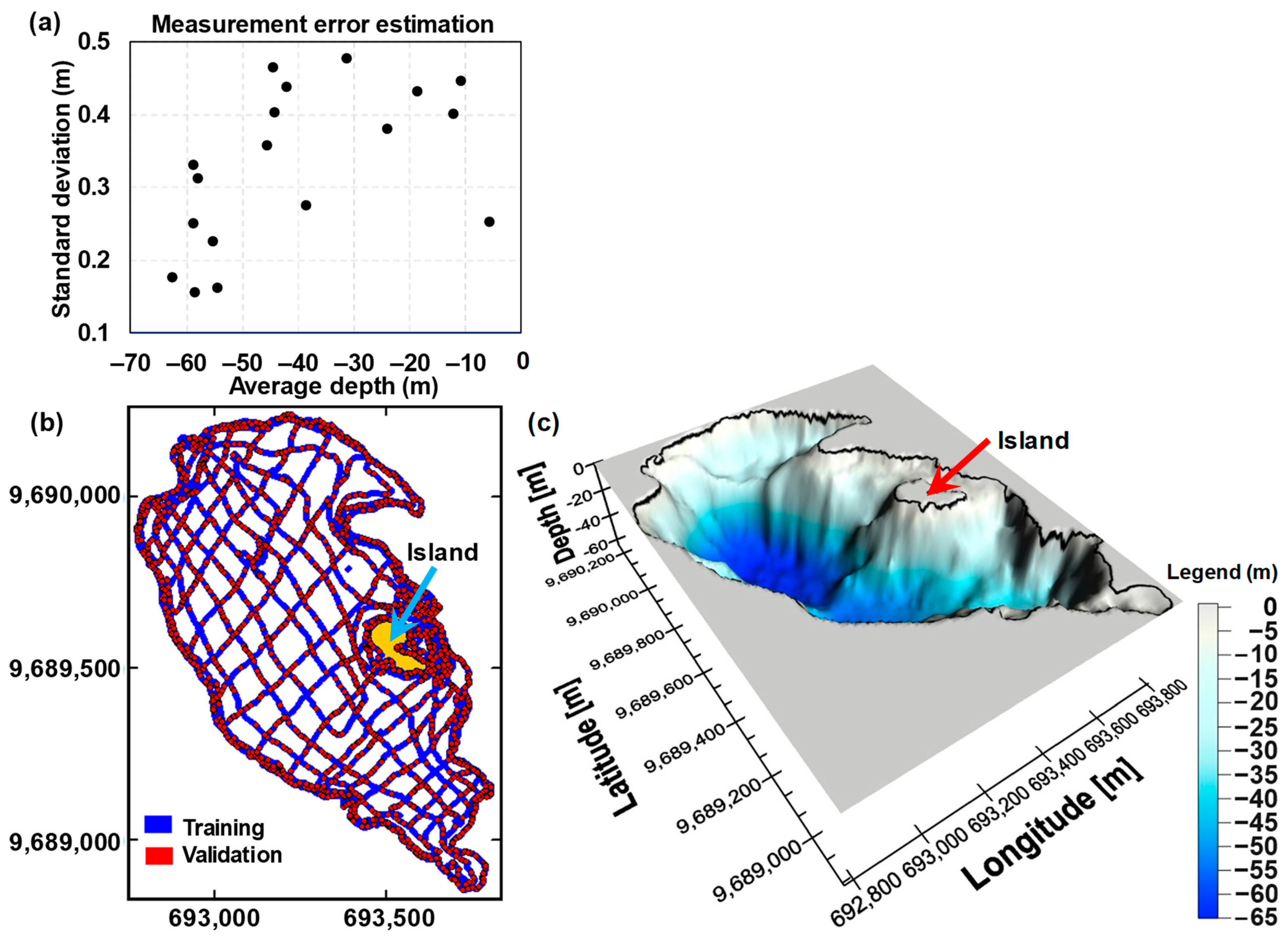
Figure 5.
Empirical exceedance probability distributions of mean absolute error (MAE) of residuals, as a function of the tried interpolation methods. Exceedance probabilities were assigned by using (a) the Weibull plotting position expression, as well as the alternative formulae (b) Blom and (c) Gringorten. Evaluation data sets were randomly selected considering different percentages of total sonar observations (i.e., 100 × (1 − Mi/Ji), see Figure 3), such as (a) 20%; (d) 30%; and (e) 40%. In the legend, numbers between parentheses in front of the names of the tested interpolation methods are the respective SURFER identifiers (SrfGridAlgorithm enumeration).
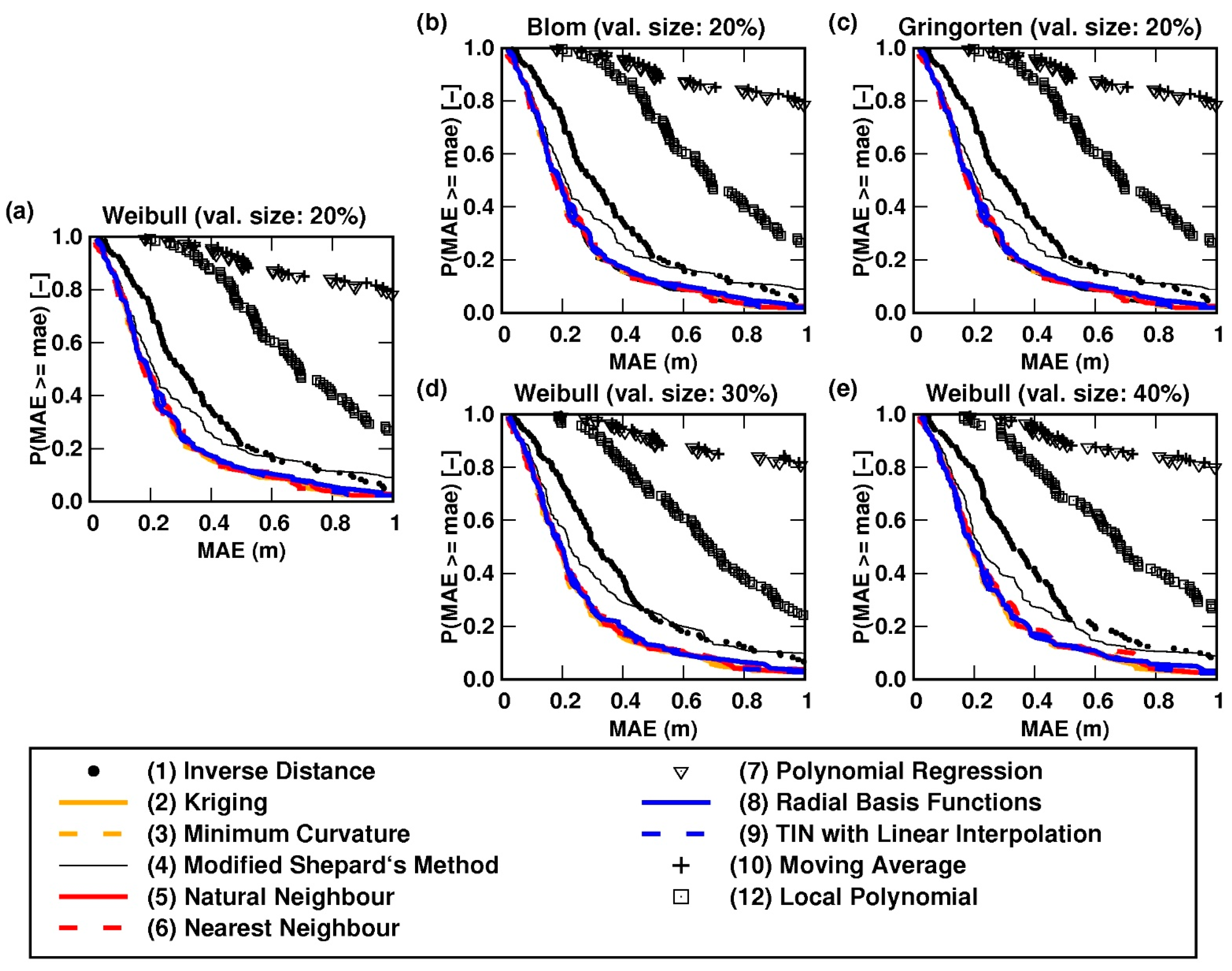
Figure 6.
Empirical exceedance probability distributions of mean absolute error (MAE) of residuals, as a function of the tried interpolation methods and the error scenarios, i.e., (a) original observations; and artificial random errors with maximum magnitudes in the order of (b) ±20 cm; (c) ±40 cm; (d) ±80 cm; (e) ±160 cm; and (f) ±320 cm. Exceedance probabilities were estimated through the Weibull plotting position expression. For every study lake, 80% of the observations were randomly selected for model training and the remaining 20% for model evaluation. In the legend, numbers in parentheses in front of the names of the tested interpolation methods are the respective SURFER identifiers.

Figure 7.
Relative hypsographic (RH) curves of lake area as a function of the vertical resolution used to determine them, i.e., (a) 0.10 m; (b) 0.25 m; and (c) 0.50 m, using products of the Kriging (ordinary) interpolation method.
Figure 7.
Relative hypsographic (RH) curves of lake area as a function of the vertical resolution used to determine them, i.e., (a) 0.10 m; (b) 0.25 m; and (c) 0.50 m, using products of the Kriging (ordinary) interpolation method.
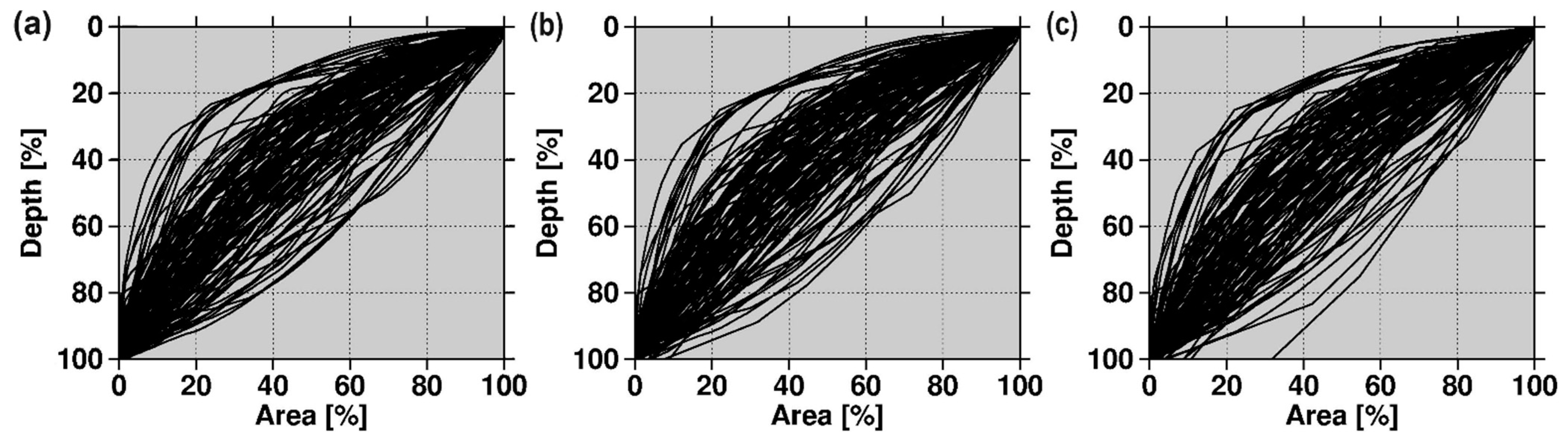
Figure 8.
Relative hypsographic (RH) curves (a) for all the study lakes within and around the Cajas National Park (CNP); (b) for the lakes with a convex form [13,14] (70% of the study lakes); (c) for the lakes with a concave form (5% of the study lakes); and (d) for the lakes with a “mixed” form (25% of the study lakes). The RH curves were determined considering a 0.1 m vertical resolution and the products of the Kriging (ordinary) method. The dashed 45° line is the reference curve that enables discretising convex and concave forms.

Figure 9.
Empirical exceedance probability distributions of mean absolute error (MAE) of residuals as a function of the average lake form: convex (70% of study lakes), concave (5% of study lakes), and mixed (25% of study lakes), for the six better-performing interpolation methods: (a) Kriging (ordinary); (b) Minimum Curvature; (c) Natural Neighbour; (d) Nearest Neighbour; (e) Radial Basis Functions (Multiquadric); and (f) TIN with linear interpolation. Empirical exceedance probabilities were estimated through the use of the Weibull plotting position expression. The size of the evaluation data set considered in the split-sample (SS) test was 20% of total sonar observations.

Figure 10.
Comparison of the DEM of the study site (a) before (original) and (b) after (enhanced) the incorporation of the bathymetric information of the Luspa lake into the DEM; (c) relative frequency; and (d) cumulative relative frequency of terrain elevation pixels, for both the original DEM and the enhanced DEM that incorporates the bathymetry of the Luspa lake. Coordinates system: UTM (m) 17-S, WGS84.

Disclaimer/Publisher’s Note: The statements, opinions and data contained in all publications are solely those of the individual author(s) and contributor(s) and not of MDPI and/or the editor(s). MDPI and/or the editor(s) disclaim responsibility for any injury to people or property resulting from any ideas, methods, instructions or products referred to in the content. |
© 2024 by the authors. Licensee MDPI, Basel, Switzerland. This article is an open access article distributed under the terms and conditions of the Creative Commons Attribution (CC BY) license (https://creativecommons.org/licenses/by/4.0/).
Share and Cite
MDPI and ACS Style
Vázquez, R.F.; Mosquera, P.V.; Hampel, H. Bathymetric Modelling of High Mountain Tropical Lakes of Southern Ecuador. Water 2024, 16, 1142. https://doi.org/10.3390/w16081142
AMA Style
Vázquez RF, Mosquera PV, Hampel H. Bathymetric Modelling of High Mountain Tropical Lakes of Southern Ecuador. Water. 2024; 16(8):1142. https://doi.org/10.3390/w16081142
Chicago/Turabian StyleVázquez, Raúl F., Pablo V. Mosquera, and Henrietta Hampel. 2024. "Bathymetric Modelling of High Mountain Tropical Lakes of Southern Ecuador" Water 16, no. 8: 1142. https://doi.org/10.3390/w16081142
Note that from the first issue of 2016, this journal uses article numbers instead of page numbers. See further details here.